The Effect of Merger Boosts on the Luminosity, Temperature, and Inferred Mass Functions of Clusters of Galaxies
Abstract
In the standard Cold Dark Matter model of structure formation, massive clusters form via the merger of smaller clusters. N-body/hydrodynamical simulations of merging galaxy clusters have shown that mergers can temporarily boost the X-ray luminosity and temperature of the merged cluster above the equilibrium values for the merged system. The cumulative effect of these “merger boosts” will affect the observed X-ray luminosity functions (XLFs) and temperature functions (TFs) of clusters. One expects this effect to be most important for the most luminous and hottest clusters. XLFs and TFs of clusters provide some of the strongest constraints on cosmological and large-scale-structure parameters, such as the mean fluctuation parameter, , and the matter density divided by the critical density, . Merger boosts may bias the values of and inferred from cluster XLFs and TFs if virial equilibrium is assumed. We use a semi-analytic technique to estimate the effect of merger boosts on the X-ray luminosity and temperature functions. The boosts from individual mergers are derived from N-body/hydrodynamical simulations of mergers. The statistics of the merger histories of clusters are determined from extended Press-Schechter (PS) merger trees. We find that merger boosts can increase the apparent number of hot, luminous clusters. For example, in a Universe with and at a redshift of , the number of clusters with temperatures keV is increased by a factor of 9.5, and the number of clusters with luminosities erg s-1 is increased by a factor of 8.9. We have used our merger-boosted TFs and XLFs to derive the cosmological structure parameters and by fitting Press-Schechter equilibrium relations to local () and distant (either or ) cluster samples. Merger boosts cause to be overestimated by about 20%. The matter density parameter may be underestimated by about 20%, although this result is less clear. If the parameters of the fluctuation spectrum are derived from the observed TF or XLF (e.g., from a low redshift sample), then this removes most of the boost effect on . However, larger merger boost effects may appear when cluster XLFs and TFs are compared to cosmological structure parameters derived by other techniques (e.g., cosmic microwave background fluctuations or the brightness of distant supernovae).
1 Introduction
Clusters of galaxies have been widely used to provide useful constraints on cosmological parameters (e.g., Henry & Arnaud 1991; Bahcall & Fan 1998; Eke et al. 1998; Borgani et al. 2001). This is in part possible because there is a well-developed theoretical framework which allows one to predict the mass function (MF) of clusters of galaxies and its evolution as a function of the cosmology. Here, the MF is defined as the number density of clusters as a function of their mass. One standard method for predicting the MF is to use Press-Schechter formalism, originally developed by Press & Schechter (1974, hereafter PS), and developed in more detail by Bond et al. (1991) and Lacey & Cole (1993), among others, in combination with the Cold Dark Matter (CDM) model. In hierarchical structure formation models like CDM, more massive halos form from the merger of smaller halos. Values of cosmological parameters can be estimated by comparing theoretical models for the MF of clusters with observations.
This technique places the strongest constraints on , the RMS mass fluctuations on a scale of Mpc where is the Hubble constant in units of km/sec/Mpc, and on , the ratio of the current mean matter density to the critical density at the current epoch (e.g., Henry & Arnaud 1991; Kitayama & Suto 1996; Eke et al. 1998; Borgani et al. 2001; Ikebe et al. 2002). Roughly speaking, the present-day abundance of clusters determines the relationship between and , while the evolution of clustering with redshift breaks this degeneracy, although Reiprich & Böhringer (2001) have been able to constrain using only a local cluster sample by assuming a CDM spectrum of perturbations whose shape parameter depends on . In these determinations, the most massive clusters have the greatest leverage. Massive clusters are rare objects, and the abundance of the most massive clusters is very sensitive to the cosmological parameters.
Unfortunately, the MF of clusters of galaxies cannot be directly observed (save by gravitational lensing in a relatively small number of cases). Generally, it is inferred from the X-ray luminosity function (XLF) or temperature function (TF), using empirical or semi-empirical relations between the masses of clusters and their temperatures () or X-ray luminosities (). These scaling relations are usually applied under the assumption that the clusters are dynamically relaxed, although in reality this cannot always be true since in the CDM model larger clusters are continually forming via mergers of smaller clusters.
Simulations have shown that if two clusters of comparable mass merge to form a larger cluster, there is a temporary increase in the cluster’s X-ray luminosity and temperature (Ricker & Sarazin 2001; Ritchie & Thomas 2002). If the cluster is observed during this period of boosted luminosity and temperature, the inferred mass will be larger than the actual mass of the cluster. In fact, such objects will be preferentially detected in X-ray flux-limited samples because they are intrinsically more luminous than equal mass clusters which are not currently experiencing a merger. This will be particularly true for X-ray selected, high redshift clusters. As a possible examples of this, one of the most distant X-ray selected clusters observed to date, RXJ1053.7+5735, has a morphology which may indicate an ongoing merger (Hashimoto et al. 2002), as does the most luminous X-ray selected cluster found to date, RXJ1347.5-1145 (Allen, Schmidt, & Fabian 2002).
If this X-ray luminosity-temperature (hereafter L-T) boost effect is sufficiently large, and if mergers occur frequently enough, then the observed XLF and TF, and hence the inferred MF, will be different from what they would be if all clusters were dynamically relaxed. One would expect that merger boosts would affect most strongly the high luminosity and temperature ends of the XLF and TF. Since the massive clusters which have very high values of and are rare, a small contribution of lower mass clusters with L-T boosts could strongly affect the statistics. As we noted above, the abundance of the hottest and most luminous clusters (which are usually assumed to be the most massive clusters) has a strong influence on the inferred values of the cosmological parameters. In particular, if merger boosts artificially increase the abundance of hot, luminous clusters at high redshift, the real value of will be underestimated. Since observations of the numbers of high temperature and luminosity clusters at moderate and high redshifts have been used to infer that is low (e.g., Bahcall, Fan, & Cen 1997; Borgani et al. 2001), this effect could be important.
In this paper we attempt to quantify the effect of mergers on the observed XLF and TF, and to determine how the X-ray L-T boost associated with mergers alters the values of and inferred from observations. We consider three possible cosmologies: an “open” model (, ), a “flat” model (), and an Einstein-de Sitter (EdS) model (, ). Here, and is the cosmological constant. We use Extended Press-Schechter (EPS) theory (§ 2) and a Monte Carlo technique to build a collection of merger histories of clusters (“merger trees,” § 3) for a variety of cosmologies. We then build two sets of XLFs and TFs from the MF given by the merger trees for each cosmology by averaging together many merger trees (§ 7). One set assumes that clusters are always relaxed when transforming from mass to temperature or luminosity (§§ 4, 7.2), while the other set includes the L-T boost effect (§ 7.3). We ignore such non-gravitational effects as preheating since such effects are mainly important for lower mass clusters and groups (Ponman et al. 1996), whereas we choose to focus on massive clusters where the effects of merger boosts are most important. We also ignore cooling flows at the centers of clusters, which may be disrupted by mergers. The disruption of cooling flows may increase the effect of mergers on X-ray temperatures, but decrease their effect on X-ray luminosities. The strength and duration of the L-T boost is estimated for arbitrary merging masses and impact parameters by interpolating and extrapolating from the results of a series of N-body/hydrodynamical simulations of binary cluster mergers (§ 5 and Appendix B). The angular momenta or impact parameters for the mergers are drawn from a distribution based on linear theory (§ 6). The boosted XLFs and TFs are presented in § 7 at a variety of redshifts, and are compared to unboosted results. The boosted and unboosted XLFs and TFs at several redshifts are fitted using a PS mass function and equilibrium relations between the mass and temperature or X-ray luminosity (§ 8). The best-fit parameters, specifically and , are compared to the “actual” parameters used to build the trees. Our conclusions are summarized in § 9.
2 Basic Press-Schechter Theory
The quantity which is given most directly by theory is the MF of clusters, , which is defined such that gives the number of clusters per unit comoving volume with masses in the range . The MF of clusters at various redshifts and for various cosmologies can be derived from numerical simulations of clustering, or from semi-analytic techniques. Since we wish to compare the effects of merger boosts on the properties of an otherwise identical ensemble of clusters in several cosmologies, it is easier to use the semi-analytical techniques. A simple expression for the mass function of clusters is given by PS formalism. Comparisons to observations of clusters and to numerical simulations show that PS provides a good representation of the statistical properties of clusters, if the PS parameters are carefully selected (e.g., Lacey & Cole 1993; Bryan & Norman 1998). Based on large N-body simulations, some authors have suggested other forms for the mass function of dark matter halos which differ somewhat from the PS predictions (e.g., Sheth & Tormen 1999; Jenkins et al. 2001). Since we are mainly interested in determining the relative effects of merger boosts on the XLF and TF, the exact form of the distribution function we assume should be unimportant, just so long as the same model is used both when including the effects of merger boosts and when ignoring them. PS formalism assumes that galaxies and clusters grow by the gravitational instability of initially small amplitude Gaussian density fluctuations generated by some process in the early Universe. The fluctuation spectrum is assumed to have larger amplitudes on smaller scales. Thus, galaxies and clusters form hierarchically, with lower mass objects (galaxies and groups of galaxies) forming before larger clusters. These smaller objects then merge to form clusters.
According to PS, the mass function of clusters is given by
| (1) |
where is the current mean density of the Universe, is the current rms density fluctuation within a sphere of mean mass , and is the critical linear overdensity for a region to collapse at a redshift .
In CDM models, the initial spectrum of fluctuations can be calculated for various cosmologies (Bardeen et al. 1986). Over the range of scales covered by clusters, it is generally sufficient to consider a power-law spectrum of density perturbations, which is consistent with these CDM models:
| (2) |
where is the present day rms density fluctuation on a scale of 8 Mpc, and is the mass contained in a sphere of radius 8 Mpc. The exponent is given by , where the power spectrum of fluctuations varies with wavenumber as ; following Bahcall & Fan (1998), we assume , which leads to throughout. The normalization of the power spectrum and overall present-day abundance of clusters is set by . The observed present-day abundance of clusters leads to (e.g., Bahcall & Fan 1998). We determine the value of by requiring that our models reproduce the observed local number density of clusters with temperature keV, which we take to be Mpc-3 keV-1 (Henry & Arnaud 1991), although some more recent observations suggest a slightly smaller value for the local number density of clusters at keV (Ikebe et al. 2002). We assume a value of km/sec/Mpc, since the results scale in a simple way with the Hubble constant. We find for the open, flat, and EdS models, respectively.
3 Merger Trees
One can determine the merger histories of clusters either moving forward in time (starting at high redshift and following the merger history of a set of subclusters) or moving backward in time (starting at present with a set of clusters, and de-merging them into subclusters). We follow the latter approach. This has several advantages. First of all, the initial populations of clusters is set at the present time, where we have the best observational data on the population of clusters. Secondly, one can start with rich clusters at present, and we don’t need to follow the evolution of low mass systems. If the merger histories are computed going forward in time, one needs to follow the histories of a large ensemble of small systems, most of which never merge into rich clusters. Since rich clusters are rare objects, this is quite inefficient.
To generate our merger trees, we follow the EPS method outlined by Lacey & Cole (1993). We begin by writing down the conditional probability that a “parent” cluster of mass at a time had a progenitor of mass in the range at some earlier time , with and :
| (3) |
Here and , with similar definitions for and . Details of the EPS theory and derivations of equation (3) are given elsewhere (see Lacey & Cole 1993; Cohn, Bagla, & White 2001).
As noted by Lacey & Cole (1993), the EPS expressions are simplified if we replace the mass and time (or redshift ) with the variables and . Note that decreases as the mass increases, and that decreases with increasing cosmic time . Let be the probability that a cluster had a progenitor with a mass corresponding to a change in of in the range at an earlier time corresponding to . Then, equation (3) becomes
| (4) |
where and .
As the mass of the progenitors is decreased (), the total number of progenitors diverges. On the other hand, the total mass associated with these progenitors converges (equation 3). Thus, it is useful to consider only progenitors with masses exceeding some minimum value . Mergers involving smaller masses are considered to be part of a continuous accretion process. In our merger trees, the masses of clusters increase continuously with cosmic time as a result of this accretion process (or decrease as we run the merger trees backwards in time). However, we do not follow the individual histories of subclusters with masses . We chose the value of .
3.1 Monte Carlo Generation of Merger Trees
We employ a Monte Carlo technique to construct merger trees. Each tree starts with a cluster with an initial mass . We step each cluster back in time, using a small but finite time step corresponding to a positive increase . We adaptively change the step size of as we run the trees backward in time by satisfying the criterion specified by Lacey & Cole (1993) that , where is the mass of the cluster at the current time step and is the smallest subcluster we wish to resolve individually. Specifically, at every step we choose a step size equal to half this maximum value. We found that using a smaller timestep equal to 1/10 of this maximum value did not significantly alter our results.
The cumulative probability distribution of subcluster masses is given by
| (5) |
where is the complementary error function. The cumulative probability distribution is defined such that as . To draw a from this probability distribution, we select a uniformly-distributed random number between 0 and 1, and determine the corresponding value of by solving numerically the equation . The value of of the progenitor is then . The mass of one of the progenitors is given by , where is given by equation (2). The mass of the other progenitor is .
Let and . If , we consider the change in mass to to be due to accretion (i.e., to a very small merger or mergers). The transitory effects of such a small merger or mergers are assumed to be small. We reduce the mass of the cluster to , where becomes the new value of for the next timestep in the merger tree. We do not follow the smaller mass as a separate subcluster. However, if , we say that a merger has occurred and we follow both of the merging subclusters of masses and separately. We continue this process until either the branch we are following drops below a mass of or we reach the maximum redshift we wish to study. We choose to run each tree back to a fixed mass limit, as opposed to a limit expressed as some fraction of the final mass , so that the mass completeness limit of the cluster sample at all redshifts can be readily determined. An example of a merger tree generated in this way is shown in Figure 1.
As pointed out by Somerville & Kolatt (1999, hereafter SK), there are some inherent problems with generating merger trees in this way. First of all, this technique allows for binary mergers only, while in reality multiple nearly simultaneous mergers are possible. SK showed that allowing for multiple mergers improves the agreement between Monte Carlo merger trees and PS theory predictions for the mass function. However, such multiple mergers mainly affect the relatively low mass halos at rather high redshifts . Since we are mainly interested in massive clusters and will only follow the merger trees out to , this is not such a significant problem here.
Another related problem with the Binary Merger Tree Method, also pointed out by SK, is that while we draw one merging halo mass from equation (5), the mass of the other merging halo is simply taken to be the mass of the progenitor minus . While this approach ensures mass conservation, it distorts the distribution function we are actually drawing halo masses from in a complicated way, such that the effective distribution is no longer described by equation (5). The solution is to continue to draw merging halo masses from equation (5) with the restriction that the sum of the halo masses does not exceed the mass of the progenitor (see SK). This requires that we allow multiple merger events.
The main reason we have not implemented this N-Branch Tree Method developed by SK is that it is unclear how to determine the luminosity and temperature boosts associated with a multiple merger event given the simulation data available (§ 5). However, it is likely that the effects of multiple mergers with smaller subclusters will be less important than major binary merger events with . In addition, we find that the predictions of our Binary Merger Tree Method agree reasonably well with PS theory over the range of redshifts and halo masses we are interested in (see § 3.3).
3.2 Ensemble of Present-Day Masses
The previous section describes how we determine the merger history of a cluster with a given mass at the present time. In order to describe the statistical properties of mergers, we construct an ensemble of such merger trees for a set of present day masses, . In principle, the simplest way to select such initial masses would be to draw them from the PS distribution at the present time, (equation 1). Then, the properties of the cluster ensemble at any redshift could be derived simply by averaging over all of the clusters in the set of merger trees. However, the PS mass function diverges at low masses (although the mass contained in the clusters converges). This means that most of the merger trees selected in this way would follow the histories of rather small clusters. In order to have enough statistics to sample the larger clusters adequately, one would require a very large number of merger trees.
In order to increase the efficiency and still have adequate statistics on large clusters, we select the initial (present day) cluster masses according to a different distribution function which gives a greater weight to higher mass systems. We draw the values of from the distribution function , which is defined such that is the number of merger trees with initial masses in the range . In practice, we take the initial masses to have logarithmically spaced masses, which corresponds to
| (6) |
where is the largest cluster mass considered, and is the total number of trees run. We construct three separate ensembles of merger trees for the three cosmologies under consideration (the open, flat, and EdS models). In each case we choose , , and a lower limit on the present day mass of clusters considered .
3.3 Test of the Merger Trees — the Mass Function
Since the method of generating merger trees described above is based on the EPS theory, we expect that the mass function produced by the merger trees will agree with the PS function (equation 1) for the same cosmological parameters. Of course, the tree-generated mass functions will be underestimated for masses smaller than , the smallest initial mass for a merger tree. The properly-weighted mass function from our ensemble of merger trees would be given by
| (7) |
where is the present age of the Universe, and the progenitor probability distribution is given in equation (3). The PS cluster mass function is defined per unit comoving volume, and the factor of weights each initial cluster and all of its progenitors by the comoving volume per cluster of mass in the Universe.
Note that the distribution of initial cluster masses cancels between the numerator and the denominator in the integral. However, we have a discrete set of initial masses, for . In the discrete limit, the integral becomes the sum , and the properly weighted mass function is
| (8) |
In the merger trees, the progenitor probability function is determined from a discrete set of progenitors for each tree. Let for be the masses of the progenitors (with masses greater than ) at redshift of the present-day cluster with a mass of . We order the progenitor masses such that We accumulate the mass function in mass bins whose boundary mass values are for , with Thus, the mass bin has a width of . Then, the tree-generated, binned mass function at redshift is given by
| (9) |
Here, is the number of progenitors at redshift of the tree with a present-day mass of that lie in the mass bin, is the smallest value of such that , and is the largest value of such that .
We compared the merger tree prediction of the MF to the PS expression (equation 1) for the ensemble of trees described in § 3.2; the comparison for the EdS model is shown in Figure 2. If equation (1) is fit to the mass function generated by the merger trees allowing and to vary the values used to construct the trees are recovered to better than 2% for and better than 7% for out to . For the EdS model, the agreement is much better: less than 2% in and roughly 2% in .
4 Non-Boosted Mass-Luminosity and Mass-Temperature Relations
The merger trees give the masses of clusters as functions of time. In order to calculate the TFs and XLFs, we need to convert cluster masses to temperatures and X-ray luminosities. We will use the bolometric X-ray luminosity in order to avoid a specific choice of an energy band. In the models including merger L-T boosts, the luminosities come from hydrodynamical simulations (§ 5); however, for comparison to the analytic PS model and to the results of merger tree simulations without merger L-T boosts, we need a set of “equilibrium” or non-boosted relations between the cluster mass and its X-ray luminosity and temperature. We could use empirical relations, but these are generally not available at all redshifts. We prefer relations which have the correct dependence on redshift and on cosmological parameters, since we consider a range of redshifts and a variety of cosmological models. Moreover, we prefer a theoretical dependence on the cluster mass rather than an empirical one, since the empirical relations may already be biased by the effects of merger boosts. It has been shown that the empirical relationship between cluster mass, luminosity, and temperature is somewhat different from what one would expect from theoretical arguments and numerical simulations where only gravitational heating is considered, even at the relatively high temperatures and luminosities we consider in this paper (e.g., Arnaud & Evrard 1999; Allen, Schmidt, & Fabian 2001; Finoguenov, Reiprich, & Böhringer 2001). At present, the detailed physics and redshift dependence of these non-gravitational effects are not well understood. As a result we did not include such effects in our simulations. While it is true that preheating and other non-gravitational effects may slightly dilute the effect of merger boosts since the fractional increase in X-ray luminosity and temperature due to mergers will be smaller if non-gravitational heating is considered, the effect will be most important for low mass clusters (Ponman et al. 1996) which are not of primary interest here. Since we are mainly interested in massive clusters, are not interested in these non-gravitational effects, and are primarily concerned with the relative effects of clusters mergers, it is preferable to use mass-temperature and mass-luminosity relations which are consistent with purely gravitational heating.
We adopt the following mass-temperature and mass-luminosity relations given by Bryan & Norman (1998):
| (10) |
| (11) |
where we have added our own normalization factors and . In these equations is the baryon density parameter and is defined as , where and is the current radius of curvature of the Universe. A fit for is given by Bryan & Norman (1998) for the relevant cosmological models:
| (12) |
where . Since our luminosity and temperature boosts have been modeled from hydrodynamical simulations we choose and so that our relations reproduce the temperature and X-ray luminosity of cluster B in Table 1 of Ricker & Sarazin (2001) (assuming cluster B is observed at ). In applying these relations to theoretical models of clusters, the redshift in equations (10) and (11) are taken to be the formation redshift of the cluster, . Once a cluster is virialized, its properties (including the temperature and luminosity) are assumed to remain constant within these equilibrium relations.
5 Merger L-T Boosts from Numerical Simulations
Using the method described in § 3.1, we are able to estimate the number of mergers occurring at a particular redshift. We also know the individual masses of the two merging halos. However, this is all the information we can get from the merger trees themselves; if we want to know about the individual cluster X-ray luminosities and temperatures, and the effect that a merger has on these quantities, we must turn to other methods.
For non-merging, virialized halos we expect a simple relationship between mass and temperature or mass and luminosity. For such halos we assume the relationships given by equations (11) and (10) throughout. However, if a cluster has recently experienced a major merger, it will be in a non-equilibrium state, and we expect its temperature and luminosity to exceed that of a relaxed cluster of equal mass at the same redshift. Since we are unaware of any verified analytic prediction of the L-T boost experienced by two merging clusters of known mass, we turn to hydrodynamical simulations of two merging clusters. The general method is to simulate a series of binary cluster mergers with varying mass ratios and impact parameters and observe the L-T boost experienced by the merged cluster in each case, and then to fit a function of the merging masses and the impact parameter to the observed L-T boosts. This fitted function is then used to determine the L-T boost associated with the merger of two clusters of arbitrary mass at any impact parameter. The details of how this fit is carried out and the results are given below in § 5.2
5.1 The Simulations
The details of the hydrodynamical simulations used to develop a model for the L-T boost are described in detail elsewhere (Ricker & Sarazin 2001). Data were available from 8 different simulation runs corresponding to three different mass ratios at three different impact parameters , excluding the one case . Here, is the scale radius of the more massive cluster, which is the parameter in the assumed Navarro, Frenk, & White (1997, hereafter NFW) mass profile of the cluster, and is defined in § 5.3. The smaller mass was fixed at for each simulation. Note that while the runs with are not mentioned specifically in Ricker & Sarazin (2001), the method used to generate them is identical to that used for the runs described therein.
5.2 Fitting Simulation Data
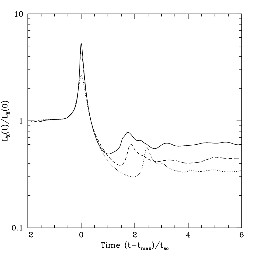
Figure 3 shows the behavior of the luminosity and temperature as a function of time for equal mass merger runs at different impact parameters (see also Ricker & Sarazin [2001], their figures 5 and 8). is the emission-weighted X-ray temperature of the merging clusters, while is the same value for the sum of the two clusters prior to the merger. Similarly, is the total X-ray luminosity of the merging clusters, while is the value prior to the merger. Note that we plot the bolometric X-ray luminosity while Ricker & Sarazin (2001) consider the X-ray luminosity in the keV band. The times are the offset from the time of peak luminosity, , and are scaled by the sound-crossing time of the more massive cluster ( is defined in § 5.3). Several peaks are evident in both the temperature and luminosity which correspond to the dense cores of the merging clusters interacting as they pass close by (or through) one another.
In applying these results to merger trees, one complication is that the merger trees treat the mergers as instantaneous, while the hydrodynamical simulations follow the mergers over time. Moreover, the merger trees are computed with a finite time resolutions (determined indirectly from ; see § 3.1). Thus, we don’t know the precise time or redshift at which each merger occurred in the merger trees. On the other hand, we are interested in the statistical effects of mergers; obviously, numerical hydrodynamical simulations are needed to follow individual mergers in detail. Thus, we assume that each merger occurred at a random time within the time resolution of the merger tree . In all cases, the time resolution of the merger trees is fine enough that there are no significant cosmological changes during a time step: for a merger which forms a 10 cluster the scale factor changes by less than 4% over one timestep, and for one which forms a 10 cluster it changes by less than 0.6%. We identify the “time” of a merger in a merger tree with the time at which the X-ray luminosity boost due to the merger is maximum (an offset time of zero in Figure 3). Generally, this corresponds to the first time the subcluster cores pass by (or through) one another.
For the purposes of determining the temperature or luminosity boost assuming the merger occurs at a random time in the merger tree time bin, it is useful to consider the distribution of cumulative times as a function of the boost. In Figure 4a, we plot the total time that the temperature exceeds some boost (scaled by the sound crossing time ) vs. the relative boost . The corresponding plots for the luminosity boost are given in Figure 4b. Of course, we are most interested in the sections of these plots which correspond to strong boosts (the right side of the plots). In Appendix B, we fit these cumulative time distributions for the numerical hydrodynamical simulations of mergers to simple analytical forms as a function of the masses of the clusters and the merger impact parameter. The parameters of these fits are interpolated or extrapolated to approximate the merger boost for mergers with arbitrary masses and impact parameters. We find that, for boosts greater than a factor of 1.5, our fits reproduce the boosts given by the hydrodynamical simulations with an average accuracy of better than 2% for the temperature boosts and 7% for the luminosity boosts . The fits are less accurate for very small boosts, but obviously these have a very small effect on the XLFs and TFs of clusters.
5.3 Application to Merger Trees
To determine the luminosity and temperature of a cluster at some observation time , we consider all the mergers the cluster has undergone prior to and the effect each merger will have on the luminosity and temperature of the cluster at . Recall that at each merger and are the masses of the less massive and more massive individual merging subclusters respectively (see § 3.1). The impact parameter of the merger is drawn from the distribution given by linear theory (see § 6 below). In the fits of the merger boosts from hydrodynamical simulations, the scaled impact parameter is used (Appendix B), where and are the core radii of the merging subclusters. Following Ricker & Sarazin (2001) and Appendix B, we take the core radius of a cluster to be 1/2 of the scaling radius . We assume a halo concentration parameter (Ricker & Sarazin 2001), where the virial radius is given by (Bryan & Norman 1998):
| (13) |
The merger boosts depend on the time elapsed since the merger, (Figure 3). As noted above, we identify the epoch of the merger in the merger tree with the time , and this time is selected at random within the (small) timestep in which the merger takes place. The times for the merger boosts are scaled by the sound crossing time of the more massive subcluster,
| (14) |
where is the sound speed in the cluster,
| (15) |
The mean mass per particle in the gas is in units of the mass of a hydrogen atom . When computing the sound speed we make the approximation that the temperature is given by equation (10), although note that Ricker & Sarazin (2001) use the central temperature when computing the sound speed.
Equation (B1) is then used with , , , and to determine the boost to the X-ray luminosity and temperature in a cluster at due to a merger at . We apply the maximum boost at from all previous mergers. Applying these relations to every cluster in the merger trees at gives a collection of luminosities and temperatures from which the XLF and the TF can be constructed as in § 7.2.
6 Angular Momenta and Impact Parameters for Mergers
The boost in X-ray luminosity and temperature during a merger depends on the impact parameter or orbital angular momentum for the merger. Unfortunately, this is not determined by the masses of the individual subclusters, and a range of values are possible for mergers of subclusters with similar masses and similar merger epochs . The merger tree simulations are based on the assumption of spherical collapse and do not give the impact parameter of the merger. In hierarchical large scale structure theories, the angular momentum is generally assumed to arise from tidal torques from surrounding material. In linear theory calculations of the growth of perturbations, the total angular momentum of a dark matter halo can be characterized by the spin parameter , defined as (Peebles 1971)
| (16) |
Here is its total energy of the dark matter halo and is its mass. In linear theory, the median value of is expected to be approximately constant, independent of the mass of the halo, and numerical simulations of large scale structure are in reasonable agreement with this approximation (e.g., Efstathiou & Jones 1979; Barnes & Efstathiou 1987; Sugerman, Summers, & Kamionkowski 2000). The median value of from linear theory and numerical simulations is . After these calculations were done we became aware of a more recent study of the distribution function of a parameter related to by Bullock et al. (2001). They propose an empirical log-normal fit to the distribution of values. Their simulations and their empirical fit are consistent with the distribution we have assumed, as long as the median value is fixed at . However, their simulations actually give a slightly smaller value of , which would slightly increase the effect of merger boosts.
Numerical simulations show that individual dark matter halos of the same mass acquire a range of different values of . We will assume that the individual components of the angular momenta of dark matter halos have a Gaussian distribution with a dispersion , which implies that the total angular momentum or spin parameter has a Maxwell-Boltzmann-like distribution,
| (17) |
where gives the probability that the spin parameter is in the range . The median value is , which gives . Figure 5 shows the distribution function predicted by equation (17) compared to the distribution measured from simulations by Bullock et al. (2001). We will assume that this distribution with applies to the total angular momentum of the merged clusters, and we draw values of at random from this distribution for each merger.
There is a simple kinematic argument which allows one to determine the impact parameter for a merger from the value of (Sarazin 2002). Let be the separation of the subcluster centers at turnaround, and let be their present separation. Then, the impact parameter is given by
| (18) |
Here, is a function of the masses of the two subclusters which is given by
| (19) |
One can show that for all masses.
If the two subclusters are treated as point masses and one assumes that they dominate the mass in their vicinity, then the turnaround separation is given by (Sarazin 2002)
| (20) | |||||
Here, is the age of the Universe at the time of the merger. In the simulations of Ricker & Sarazin (2001), the impact parameter is set at the start of the simulations, when the separation of the two subclusters is
| (21) |
where and are the cutoff radii of the two clusters (Ricker & Sarazin 2001).
7 Results: Luminosity and Temperature Functions
7.1 Press-Schechter Non-Boosted Prediction
For the purposes of comparison to our merger tree results, both with and without merger boosts, it is useful to have a simple prediction of the XLF and TF based on the PS mass function. The XLF and TF of virialized, non-merging clusters at an observed redshift can be approximated by combining the PS mass function (equation 1) with the mass-luminosity (equations 11) or mass-temperature (equations 10) relation. Note that these relations depend on the redshift at which each cluster was formed. Once a cluster is virialized, its temperature and luminosity are assumed to remain constant. For clusters of a given mass observed at some redshift , we need to know the formation redshift . For the merger-tree models, we can calculate from the merger histories. However, the formation redshift is not uniquely determined by the mass and observed redshift of a cluster. A common approximation has been to assume that the formation redshift is approximately the observed redshift, . However, this turns out to be inadequate to fit our merger tree results without merger boosts.
We have taken the formation redshifts of different clusters of mass observed at redshift to be equal to the mean for each (,), as determined by Lacey & Cole (1993) using the parameterization
| (22) |
The quantities and were defined in § 3; and are the values at the time of the observation, while and are the values at the epoch of the cluster formation. Cluster formation is assumed to occur when a subcluster has a mass which is greater than or equal to one half the mass of the cluster at the time of observation, so that . So that we will be able to directly compare our analytic luminosity and temperature functions to the merger tree results, we adopt a mean value of from our own merger trees. We find a mean value , which is in good agreement with the mean of the distribution given by Lacey & Cole (1993, see their Figure 9).
Combining equation (1) with equations (10) and (11) gives us analytic expressions for the XLF and TF:
| (23) |
| (24) |
The TF is defined so that gives the number of clusters per unit comoving volume with temperatures in the range (similarly for the XLF ). The mass-temperature relation and mass-luminosity relation are given by equations (10) and (11), respectively. The formation redshift is determined by solving equation (22) for with , and then converting to .
7.2 Merger Tree Prediction Without Merger Boosts
The XLF and TF of clusters can be extracted from the merger trees using the method described in § 3.3. The temperature function in bins is given by equation (9) if we replace with , and if is the number of cluster progenitors with temperatures in the temperature bin. The luminosity function is given by the same expression, replacing with , the luminosity bin. We select an observation time or redshift , identify the collection of progenitor masses which exist in the merger trees at that time, transform this collection of masses into a collection of temperatures or luminosities using equation (10) or (11), and then apply the appropriate form of equation (9). A comparison of the TF given by equation (23) to that given by the merger trees is shown in Figure 6 for an EdS Universe. The merger tree curves lie slightly above the analytic predictions, even at . This discrepancy seems to be related to the approximation used to determine the formation redshifts of clusters when determining the PS TF and XLF using equations (10) and (11); we assumed throughout, whereas in reality there is a distribution of formation redshifts for a fixed cluster temperature and luminosity. In general, this distribution is somewhat skewed (e.g. Kitayama & Suto 1996) so that convolving it with the PS distribution may produce a different TF from the one obtained if an average formation epoch is assumed. If, as a test, we set in the merger trees and in equation (23), the agreement between the curves in Figure 6 is improved.
7.3 Merger Tree Predictions With Merger Boosts
It is interesting to compare the XLFs and TFs given by the merger trees when the effects of merger boosts are included to those given when merger boosts are ignored. Figures 7 and 8 plot the boosted and unboosted merger tree TFs and XLFs, respectively, for the three cosmologies under consideration. At low temperatures ( keV) and luminosities ( erg/sec), there is good agreement between the unboosted and boosted curves. However, at larger temperatures and luminosities, the boosted XLFs and TFs rise above the unboosted curves. This is due to the fact that majors mergers with large boosts are relatively rare events. Thus, they do not affect the statistics of clusters unless the virialized clusters with the same temperature and luminosity are themselves extremely rare. There is an exponential drop-off in the expected number of the most massive clusters (equation 1), which have the largest virialized temperatures and luminosities. Thus, relatively rare major mergers of smaller and more common clusters can compete with the numbers of these most massive clusters.
Table 1 gives the fractional increase in the cumulative luminosity and temperature functions at due to merger boosts for the three cosmologies we consider. For example, in the flat model at , merger boosts cause the number of clusters with temperatures keV to increase by a factor of 9.49, and the number of clusters with luminosities erg s-1 is increased by a factor of 8.9. The same factors for the EdS model at a redshift of are 37.7 and 24.1 for the cumulative temperature and luminosity functions respectively. We note that the increase in the boosted XLFs and TFs over the unboosted values is largest in the EdS model, weakest in the open model, and intermediate in the flat model. This is to be expected since the evolution of cluster abundance is relatively rapid in the EdS model, less rapid in the flat model, and least rapid in the open model. This means that at low redshifts, the merger rate must be highest in the EdS model and lowest in the open model. In fact, the evolution of the cluster abundance is so rapid in the EdS model that the higher temperature and luminosity clusters have essentially disappeared by a redshift of one. For this reason, we adapt lower temperature and luminosity limits for the EdS model at in Table 1.
It should be noted that at the highest temperatures and luminosities the merger tree predictions are uncertain for non-zero redshifts since there are fewer and fewer hot luminous clusters at larger and larger redshifts, so that the statistics in the high end bins are poor. This effect is most noticeable in the EdS model where cluster abundance evolution occurs most rapidly so that high mass, high redshift objects are especially rare. For example, the large discrepancy at keV and between the boosted and unboosted TFs for the EdS model seen in Figure 7 is not a real effect but an artifact of the lack of high temperature clusters at this redshift.
Note that merger boosts cause keV clusters at in an EdS model to be almost as common as in the flat model. Thus, if all of the cosmological parameters other than were known from other measurements, and the abundance of very hot or very X-ray luminous clusters at high redshift were used to determine , the value would be substantially underestimated.
8 Fitting Merger Tree Data
We now treat the binned XLFs and TFs generated from the merger trees as we would observational data, fitting the data with equations (23) and (24) and treating and as free parameters of the fit. The models are fit using least squares fitting, where we choose to minimize the square of the difference of the logs of the PS and merger tree TFs and XLFs so that more weight is given to hot, luminous clusters. If we only consider observations at one redshift, there is a degeneracy between the fitting parameters and , such that (e.g., Bahcall & Fan 1998). One way to break this degeneracy is to simultaneously fit data at two or more redshifts. For each of the three cosmologies under consideration, we have simultaneously fit the TFs and XLFs at and at either or . This corresponds to the typical procedure of using observations of a low redshift cluster sample to determine the local TF or XLF (and possibly infer the mass function), and then comparing to a higher redshift sample.
The merger boosted TFs and XLFs for the models are shown in Figures 9 and 10 along with best-fit PS models. The best-fit parameters found in fitting equations (23) & (24) to the boosted and unboosted temperature and luminosity functions of the merger trees are given in Tables 2 & 3. For comparison, the actual values of the parameters used to build the merger trees are also given in these tables.
If we compare the values given for from the boosted TFs and XLFs to those given by the unboosted functions we see that, in general, merger boosts cause to be overestimated by about 20% (except for the open model XLF, which only shows a 5% increase). Similarly, if we compare the values of from the unboosted TFs to the values actually used to construct the trees, we find that they are about 10% larger. The same comparison for the XLF results also show that is larger than the original values used to build the merger trees, but there is a lot of scatter in the magnitude of the increase. The unboosted values are systematically higher than the original values because the merger tree TFs and XLFs lie slightly above the curves given by equations (23) & (24) with the original values of and . As mentioned in § 7.2, this has to do with the fact that the formation times must be estimated when using equation (23), whereas for the merger trees we have a record of the formation time for each cluster. A similar set of comparisons shows that, in the case of the TFs, merger boosts cause to be underestimated by about 20%, while the unboosted values for are smaller than the actual values used to build the merger trees by about 15%. The XLF results for show large variations and no systematic trends. Thus, while the results from the TFs suggest that merger boosts can cause to be underestimated by about 20%, the results from the XLFs are less conclusive.
It should be noted that the effect of merger boosts on and depends somewhat on the detailed method used to determine the TFs and XLFs and the criteria used to fit them. Thus, the results given here should be viewed as an illustration. Since the merger boost effect is greatest for the highest temperatures and luminosities, the effect on and will be greatest for samples of hot, luminous clusters, or for fitting techniques that weight these clusters more highly.
While much of the work done to date on using the XLF and TF of clusters to constrain both and has used the evolution of these functions to break the degeneracy between them, it should be noted that some recent studies simultaneously determine these two parameters using only the shape of the local mass function of clusters (e.g., Reiprich & Böhringer 2001). This study relies on the predicted variation of the fluctuation spectrum with in CDM models. Since we assume a power-law fluctuation spectrum, we cannot compare directly to the results of Reiprich & Böhringer (2001). However, we did perform a series of fits using only the local data from the merger trees to determine the relative effects of merger boosts on the derived cosmological parameters. The results are consistent with the results obtained by simultaneously fitting local and higher redshift merger tree data as discussed above.
9 Discussion and Conclusions
Hydrodynamical simulations of binary cluster mergers have shown that mergers can temporarily boost the X-ray luminosity and temperature of the merged cluster beyond their virial equilibrium values. These merger boosts can alter the observed TFs and XLFs of clusters, particularly at the high ends. Even a few “extra” clusters with high luminosities and temperatures can have a significant impact due to the relative rarity of massive clusters. The mass function of clusters is commonly inferred from the observed TF or XLF, assuming virial equilibrium. The inferred mass function is often used to constrain cosmological parameters. Thus, merger boosts can affect the inferred cosmological parameters.
We tested the amplitude of the merger boost effect by using EPS theory and a Monte Carlo technique to numerically reconstruct the merger histories (trees) of a population of clusters. At each merger, we quantified the strength of the merger boost by extrapolating or interpolating from a set of hydrodynamical simulations of cluster mergers. We then built TFs and XLFs from the merger trees, averaging together our sets of merger histories so that the sample cluster population was representative of the observed present day population.
Our results show that merger boosts do indeed affect the apparent number of high mass clusters. For example, in the flat model at merger boosts cause the number of clusters with temperatures keV to increase by a factor of 9.5, and the number of clusters with luminosities erg s-1 is increased by a factor of 8.9. The effect is strongest for an EdS model, since clusters evolve more rapidly in this model than in the open and flat models. In the EdS model at a redshift of , the number of clusters with temperatures keV is increased by a factor of 38, and the number with luminosities erg s-1 by a factor of 24. At first this might appear contradictory with the fact that the X-ray luminosity receives a larger boost from mergers than the X-ray temperature (see Figure 3). However, the range of X-ray luminosities is larger than the range of X-ray temperatures; another way of saying this is that the X-ray luminosity-temperature relationship is much steeper than linear. At a result, the overall effect of luminosity boosts on the XLF is not as strong as the effect of temperature boosts on the TF.
Comparing the boosted and unboosted differential TF for the EdS and flat models at shows that merger boosts cause keV clusters to be almost as common in the EdS model as in the flat model. This means that if all cosmological parameters other than were known from other measurements, and the abundance of very hot or very X-ray luminous clusters at high redshift were used to determine , the value would be substantially underestimated.
We fit PS distributions to our simulated TFs and XLFs. We did this by considering two samples: a low redshift, local sample (), and a moderate or high redshift sample ( or ). The two samples are fit simultaneously to determine the best-fit values of and , and these values were compared to the actual values used to construct the merger trees. Merger boosts can cause to be overestimated by about 20%. Merger boosts may also cause to be underestimated by about 20%, although the results from the XLF fits do not show a clear trend. The effect of merger boosts on the inferred value of is much smaller in these fits than might have been expected from the overall increase in the number of hot clusters at high redshifts produced by merger boosts. Much of the effect of merger boost is “renormalized” away by the joint fit of low and high redshift sample. One way to think of this is that merger boosts increase the numbers of hot clusters, both at low redshift and high redshift. Determining from the low redshift sample or from a joint fit removes much of the boost effect, and the change in is smaller than one might have expected.
Studies of the abundance of hot or luminous clusters at high redshift have been used to argue that we live in a low density Universe (e.g., Bahcall & Fan 1998; Borgani et al. 2001). It would appear that merger boosts do not invalidate this conclusion, although the error bars should be increased significantly to include the systematic uncertainties associated with merger boosts.
On the other hand, merger boosts do affect the value of . As noted before, the number of the hottest and most luminous clusters are affected quite strongly. Thus, any comparison between cluster TFs and XLFs and cosmological parameters derived from other objects (from cosmic microwave background radiation fluctuations, or from the brightness of distant supernovae) is likely to be inconsistent and may lead to errors in the deduced cosmological parameters. At the least, the systematic uncertainties are likely to be much larger than might be inferred from the statistics of clusters alone.
Obviously, the effect of merger boosts could be avoided entirely if the mass function could be determined directly from gravitational lensing observations. Radio detections of the Sunyaev-Zel’dovich (SZ) effect can also provide a measure of the number of luminous and hot clusters, particularly at high redshift (e.g., Holder et al. 2000). Although mergers should also boost the microwave decrement from clusters, we expect that this effect would be smaller than the effect on the X-ray emission-weighted temperature or the X-ray luminosity, because the SZ effect depends on density rather than the square of the density.
References
- (1)
- (2) Allen, S. W., Schmidt, R. W., & Fabian, A. C. 2001, MNRAS, 328, L37
- (3)
- (4) Allen, S. W., Schmidt, R. W., & Fabian, A. C. 2002, MNRAS, in press (astro-ph/0111368v2)
- (5)
- (6) Arnaud, M., Evrard, A. E. 1999, MNRAS, 305, 631
- (7)
- (8) Bahcall, N. A., Fan, X., & Cen, R. 1997, ApJ, 485, 53
- (9)
- (10) Bahcall, N. A., & Fan, X. 1998, ApJ, 504, 1
- (11)
- (12) Bardeen, J. M., Bond, J. R., Kaiser, N., & Szalay, A. S. 1986, ApJ, 304, 15
- (13)
- (14) Barnes, J., & Efstathiou G. 1987, ApJ, 319, 575
- (15)
- (16) Bond, J. R., Cole, S., Efstathiou, G., & Kaiser, N. 1991, ApJ, 379, 440
- (17)
- (18) Borgani, S., et al. 2001, ApJ, 561, 13
- (19)
- (20) Bryan, G. L., & Norman, M. L. 1998, ApJ, 495, 80
- (21)
- (22) Bullock, J. S., Dekel, A., Kolatt, T. S., Kravtsov, A. V., Klypin, A. A., Porciani, C., & Primack, J. R. 2001, ApJ, 555, 240
- (23)
- (24) Cavaliere, A., & Fusco-Femiano, R. 1976, A&A, 49, 137
- (25)
- (26) Cohn, J. D., Bagla, J. S., & White, M. 2001, MNRAS, 325, 1053
- (27)
- (28) Efstathiou, G., & Jones, B. J. T. 1979, MNRAS, 186, 133
- (29)
- (30) Eke, V. R., Cole, S., Freml, C. S., & Henry, J. P. 1998, MNRAS, 289, 1145
- (31)
- (32) Finoguenov, A., Reiprich, T. H., & Böhringer, H. 2001, A&A, 368, 479
- (33)
- (34) Hashimoto, Y., Hasinger, G., Arnaud, M., Rosati, P., & Miyaji, T. 2002, A&A, 381, 841
- (35)
- (36) Henry, J. P., & Arnaud, K. A. 1991, ApJ, 372, 410
- (37)
- (38) Holder, G. P., Mohr, J. J., Carlstrom, J. E., Evrard, A. E., & Leitch, E. M. 2000, ApJ, 544, 629
- (39)
- (40) Ikebe, Y., Reiprich, T. H., Böhringer, H., Tanaka, Y., & Kitayama, T. 2002, A&A, 383, 773
- (41)
- (42) Jenkins, A., et al. 2001, MNRAS, 321, 372
- (43)
- (44) Kitayama, T., & Suto, Y. 1996, ApJ, 469, 480
- (45)
- (46) Lacey, C., & Cole, S. 1993, MNRAS, 262, 627
- (47)
- (48) Navarro, J. F., Frenk, C. S., & White, S. D. M. 1997, ApJ, 490, 493 (NFW)
- (49)
- (50) Peebles P. J. E. 1971, A&A, 11, 377
- (51)
- (52) Peebles P. J. E. 1980, The Large-Scale Structure of the Universe (Princeton: Princeton Univ. Press)
- (53)
- (54) Ponman, T. J., Bourner, P. D. J., Ebeling, H., & Böhringer H. 1996, MNRAS, 283, 690
- (55)
- (56) Press, W. H., & Schechter, P. 1974, ApJ, 187, 425
- (57)
- (58) Reiprich, T. H., & Böhringer H. 2001, ApJ, 567, 716
- (59)
- (60) Ricker, P. M., & Sarazin, C. L. 2001, ApJ, 561, 621
- (61)
- (62) Ritchie, B. W., & Thomas, P. A. 2002, MNRAS, 329, 675
- (63)
- (64) Sarazin, C. L. 2002, in Merging Processes in Clusters of Galaxies, ed. L. Feretti, I. M. Gioia, & G. Giovannini (Dordrecht: Kluwer), in press (astro-ph/0105418)
- (65)
- (66) Sheth, R. K., & Tormen, G. 1999, MNRAS, 308, 119
- (67)
- (68) Somerville, R. S., & Kolatt, T. S. 1999, MNRAS, 305, 1
- (69)
- (70) Sugerman, B., Summers, F. J., & Kamionkowski, M. 2000, MNRAS, 311, 762
- (71)
Appendix A Cosmological Dependence of
The critical overdensity as a function of cosmic time depends on the cosmological parameters and . In this paper we use the following expressions for :
| (A1) |
For the open model (, ), represents the epoch at which a nearly constant expansion takes over and no new clustering can occur, and the growth factor can be expressed as
| (A2) |
where is the standard parameter in the cosmic expansion equations (Peebles 1980, eqn. 13.10)
| (A3) |
A similar set of relations holds for the closed model (, ):
| (A4) |
| (A5) |
In this model represents the lifetime of the Universe, that is to say the cosmic time at which the Universe formally recollapses to a singularity. Although we do not consider a closed cosmological model when building merger trees it is necessary that our fitting routines be able to consider cosmologies with when fitting cosmological parameters to the merger tree data (see § 8). The solution for in the Einstein-de Sitter model can be obtained from the open model solution by the limit (Lacey & Cole 1993). To evaluate in the flat model ), we have used an approximation given by Kitayama & Suto (1996). Here is the value of the mass density ratio at the redshift of formation,
| (A6) |
In this model the growth factor can be written as
| (A7) |
(Peebles 1980, eqn. 13.6) where and .
Appendix B Fitting Simulation Data
As described in § 5.2, we wish to fits the portions of the histograms shown in Figure 4 which correspond to strong boosts. We find that these portions of the cumulative time distribution are well described by hyperbolas of the form
| (B1) |
The parameters in this function are the largest temperature boost during the merger , the duration of the period of maximum temperature boost , and which describes the eccentricity of the hyperbola. As similar expression fits the time distribution of luminosity boosts, with parameters , , and .
After fitting the function given by equation (B1) to each of the luminosity and temperature boost histograms shown in Figure 4, we determined the dependence of the boost histogram parameters on the kinematics of the merger. We characterize the merger kinematics by two dimensionless parameters. The first is the fractional mass increase in the merger, . Following the discussion in above, let be the smaller of the two masses of the merging subclusters and be the larger of the two masses. Then, . Our second parameter is the impact parameter for the merger, divided by the sum of the core radii of the two merging subclusters, . Here, and are the core radii of the merging subclusters, which are taken to be 1/2 of the scaling radius for each subcluster.
We find that the variation of the boost histogram parameters with the merger kinematics can be fit with the following functions (for the temperature boost):
| (B2) |
| (B3) |
| (B4) |
where and are in units of . Similar expressions are used for the X-ray luminosity boost. The best-fit parameters in these fits are listed in Table 4.
Note that equation (B2) implies that the temperature and luminosity boosts are largest for equal mass mergers (), and go to zero as the mass of the smaller subcluster goes to zero (). Similarly, equation (B3) implies that the histogram becomes a vertical line as ; that is, all of the time is spent with no boost. As the mass fraction increases, decreases, and the boost histogram becomes more extended toward large boosts. The dependence of the maximum boost (equation B2) and eccentricity (equation B3) on impact parameter is based on the assumption that the gas distributions in clusters are well-fit by the standard beta model (Cavaliere & Fusco-Femiano 1976), and that the strength of the boost depends on the degree of interactions of the densest portions of the two subclusters. Thus, equations (B2) & (B3) give the largest boost for a nearly head-on collision, and the boost goes to zero as the impact parameter increases. The quadratic dependence on reflects the form of the density dependence in the beta model.
The form we adapted for the variation in the time duration of the merger boost (equation B4) follows from simple scaling for the time scales for mergers. Assuming that the two subclusters have fallen from a large distance to a separation , their relative velocity is
| (B5) |
where we approximate the subclusters as point masses. The time scale for the merger boost is given by . For a given formation epoch, the core radii and other length scales associated with clusters scale as . Thus, we assume that the subcluster separation during the time of maximum merger boost scales as . One might expect that boost time to scale roughly as
| (B6) |
The virial relation for the temperature of the gas in clusters leads to , which implies that the sound-crossing time is nearly independent of mass. These arguments determine the mass dependence of equation (B4). If these arguments held exactly, we would expect . Although the best-fit values are close to this (Table 4), the fits are improved if is allowed to vary. We adapt the same dependence on as in the other fits.
Ultimately these fits will be used to determine the luminosity and temperature boosts associated with a pair of merging halos given the time during the merger at which the merging cluster is observed. For a given value of , equations (B1), (B2), (B3), & (B4) and the parameters in Table 4 reproduce the temperature boosts with an average accuracy of better than 2% for all boosts greater than 1.5. The accuracy of the fit typically increases with the strength of the boost; thus the accuracy for the strongest temperature boosts are generally better than 1%. The fits for the luminosity boosts have an average accuracy better than 7% for boosts greater than 1.5.
| Fractional Increase in Number of Clusters | |||||
|---|---|---|---|---|---|
| Model | keV) | keV) | |||
| Open | 0.0 | 1.96 | 2.35 | 1.97 | 3.43 |
| Open | 0.5 | 2.24 | 4.64 | 1.71 | 4.97 |
| Open | 1.0 | 2.32 | 3.30 | 1.71 | 3.91 |
| Flat | 0.0 | 2.10 | 2.24 | 2.01 | 4.37 |
| Flat | 0.5 | 2.56 | 3.54 | 2.04 | 8.11 |
| Flat | 1.0 | 3.37 | 9.49 | 2.05 | 8.90 |
| EdS | 0.0 | 2.73 | 5.62 | 4.08 | 20.7 |
| EdS | 0.5 | 11.3 | 37.7 | 4.51 | 24.1 |
| EdSaaFor the EdS model at , we use minimum values of keV, keV, erg s-1, and erg s-1. | 1.0 | 3.25 | 6.72 | 2.65 | 21.7 |
| Model | Redshifts | ||||||
|---|---|---|---|---|---|---|---|
| Open | 0,0.5 | 0.8274 | 0.3 | 0.913 | 0.26 | 1.190 | 0.13 |
| Open | 0,1.0 | 0.8274 | 0.3 | 0.912 | 0.26 | 1.046 | 0.21 |
| Flat | 0,0.5 | 0.8339 | 0.3 | 0.919 | 0.25 | 1.096 | 0.20 |
| Flat | 0,1.0 | 0.8339 | 0.3 | 0.905 | 0.26 | 1.095 | 0.20 |
| EdS | 0,0.5 | 0.5138 | 1.0 | 0.555 | 0.86 | 0.667 | 0.71 |
| EdS | 0,1.0 | 0.5138 | 1.0 | 0.575 | 0.77 | 0.693 | 0.63 |
Note. — The subscript “a” indicates the actual values used to construct the trees, “nb” indicates the fitted parameters for the unboosted temperature merger tree functions, and “b” indicates the fitted parameters to the boosted temperature functions.
| Model | Redshifts | ||||||
|---|---|---|---|---|---|---|---|
| Open | 0,0.5 | 0.8274 | 0.3 | 1.057 | 0.49 | 1.113 | 0.38 |
| Open | 0,1.0 | 0.8274 | 0.3 | 1.085 | 0.59 | 1.145 | 0.46 |
| Flat | 0,0.5 | 0.8339 | 0.3 | 0.857 | 0.19 | 1.037 | 0.37 |
| Flat | 0,1.0 | 0.8339 | 0.3 | 0.849 | 0.17 | 1.000 | 0.23 |
| EdS | 0,0.5 | 0.5138 | 1.0 | 0.535 | 0.82 | 0.655 | 1.20 |
| EdS | 0,1.0 | 0.5138 | 1.0 | 0.546 | 0.99 | 0.638 | 0.93 |
| Boost | A | B | C | D | E | F | G | H | I |
|---|---|---|---|---|---|---|---|---|---|
| 195 | 0.448 | 49 | 132 | 0.539 | 127 | 349 | 2.81 | 94 | |
| 240 | 0.659 | 29 | 92 | 0.316 | 84 | 96 | 3.29 | 129 |