Shear-Driven Field-Line Opening and the Loss of a Force-Free Magnetostatic Equilibrium

Abstract

This paper discusses a quasi-static evolution of a force-free magnetic field under slow sheared footpoint motions on the plasma’s boundary, an important problem with applications to the solar and accretion disk coronae. The main qualitative features of the evolution (such as field-line expansion and opening) are considered and a comparison is made between two different geometrical settings: the Cartesian case with translational symmetry along a straight line, and the axisymmetric case with axial symmetry around the rotation axis. The main question addressed in the paper is whether a continuous sequence of force-free equilibria describes the evolution at arbitrarily large values of the footpoint displacement or the sequence ends abruptly and the system exhibits a loss of equilibrium at a finite footpoint displacement. After a formal description of the problem, a review/discussion of the extensive previous work on the subject is given. After that, a series of simple scaling-type arguments, explaining the key essential reason for the main qualitative difference between the two geometry types, is presented. It is found that, in the Cartesian case, force-free equilibria exist at arbitrarily large values of shear and the field approaches the open state only at infinite shear, whereas in the axisymmetric case the field opens up already at a finite shear.

1 Introduction and Geometrical Settings

In studies of force-free coronal magnetic fields in solar physics, as well as in a closely related and essentially very similar problem of accretion disk magnetospheres, there has been some controversy regarding the issue of the loss of equilibrium. This controversy has arisen from the problem of finding a continuous sequence of force-free equilibria in the corona, invoked to represent a time evolution of the coronal magnetic field under slow plasma motions in the Sun’s photosphere. Indeed, the footpoints of the magnetic field lines are frozen into the photosphere and hence the photospheric motions lead to continuous shearing of the magnetic field. Under the assumption of ideal magnetohydrodynamics (MHD), if these motions are much slower than the Alfvén velocity in the corona (an assumption justified by a very low plasma density in the corona), the coronal magnetic field progresses through a sequence of equilibria. An important aspect of the problem is that the domain under consideration is infinite, so that the field lines can expand freely into space, instead of being confined to a finite-size box.

When trying to build a theoretical model of this process, one typically starts with a potential (no shear) field, and then gradually increases the shear. This initial potential field is taken to be closed, which means that both footpoints of each field line lie on the surface, i.e., no field line extends to infinity. The critical question then is whether one should be able to find a force-free equilibrium configuration (with the same topology as that of the original potential field) as the shear is increased indefinitely, or one should reach a certain critical point, beyond which no same-topology equilibrium solutions can be found (loss of equilibrium).

Even though this question has first been tackled in the context of the solar corona, a very similar process has also been investigated in the context of accretion disk coronae, where the sheared footpoint motion arises naturally from the differential rotation of a Keplerian disk or from the relative star–disk rotation (see van Ballegooijen 1994; Goodson et al. 1999; Uzdensky et al. 2002; Lovelace et al. 1995; Uzdensky 2002).

In either context, some simplifying assumptions are usually made in order to make the problem tractable. One of the most important is the assumption that there is one ignorable direction on the photospheric surface, i.e., a direction along which the fields are constant. There are two different symmetry classes that are most often studied:

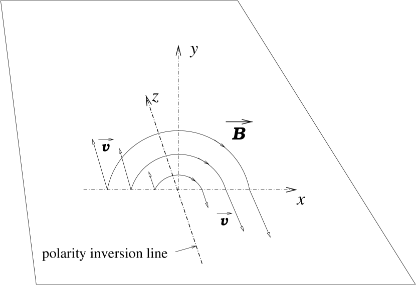
Figure 1: Cartesian geometry with translational symmetry along the polarity inversion line (the $z$ axis); vector ${\bf v}$ represents the footpoint displacement along this line.

1) Cartesian (or plane) geometry (see Fig. 1), the photosphere being an infinite plane and the corona — a half-space above this plane. The field line topology is that of a straight line dipole placed on or somewhere beneath the plane. The footpoints are displaced along the line dipole axis (also called the polarity inversion line) and the system possess translational symmetry along this axis. This problem is usually studied in Cartesian coordinates, with the ignorable direction (the line dipole axis) denoted by, say, $z$ and the direction perpendicular to the plane by $y$. There have been extensive analytical (Low 1977, 1982, 1990; Birn et al. 1978; Priest & Milne 1980; Birn & Schindler 1981; Aly 1984, 1985, 1990, 1993, 1994; Priest & Forbes 1990) and numerical studies of this problem. The latter can be subdivided further into numerical computations of sequences of force-free equilibria (Sturrock & Woodbury 1967; Jockers 1978; Klimchuk et al. 1988; Klimchuk & Sturrock 1989; Finn & Chen 1990; Wolfson & Verma 1991) and full MHD numerical simulations (e.g., Biskamp & Welter 1989; Amari et al. 1996a).

2) axisymmetric geometry, with axial (or cylindrical) symmetry around the $z$ axis ($\phi$-direction). This case is usually treated in either cylindrical ($\rho,z,\phi$) or spherical ($r,\theta,\phi$) coordinates. The footpoints rotate in the azimuthal (or toroidal) direction $\phi$. The problem has been considered both analytically (Aly 1984, 1991, 1993, 1995; Low 1986; van Ballegooijen 1994; Lynden-Bell & Boily 1994; Sturrock et al. 1995; Wolfson 1995; Uzdensky et al. 2002; Uzdensky 2002) and numerically (Barnes and Sturrock 1972; Yang et al. 1986; Porter et al. 1992; Wolfson & Low 1992; Roumeliotis et al. 1994; Mikić and Linker 1994; Uzdensky et al. 2002).

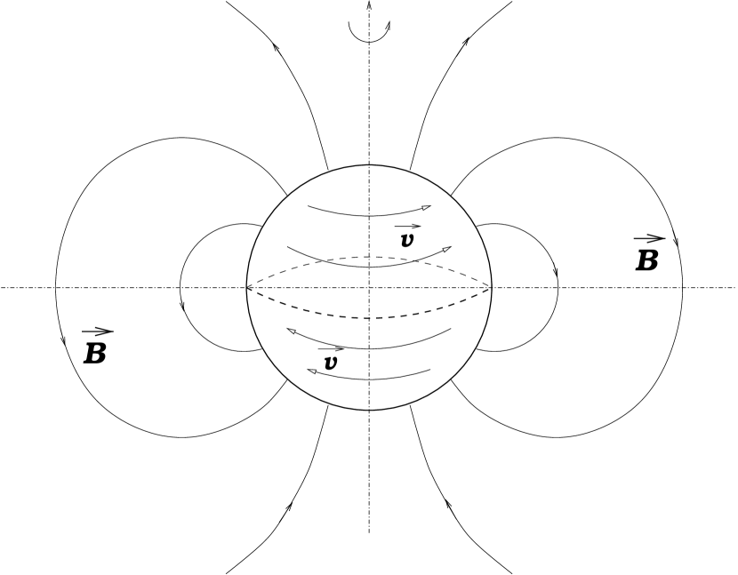
Figure 2: Spherical geometry: axisymmetric dipole-like field outside a sphere. The azimuthal displacement of the footpoints on the sphere is represented by ${\bf v}$.

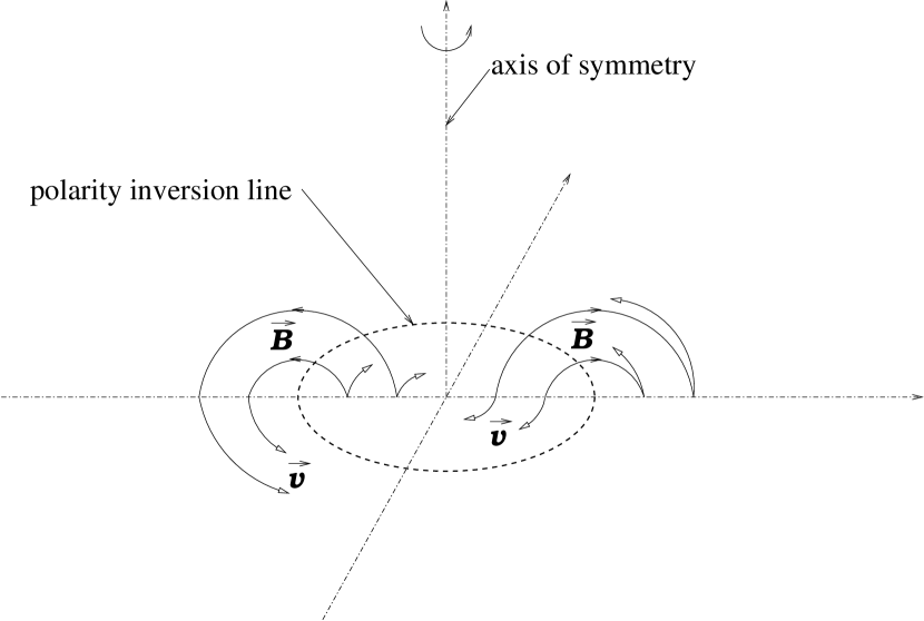
Figure 3: Cylindrical geometry with axial symmetry around the vertical axis. The magnetic field comes out of the plane $z=0$ inside the circular polarity inversion line and goes back into this plane outside this line. The azimuthal displacement of the footpoints on the plane is represented by ${\bf v}$.

One should be aware that the are actually two distinct geometrical settings in the axisymmetric case. One (which we shall call spherical geometry) is where the domain if interest is the outside of a differentially rotating sphere, with all the footpoints fixed on the surface of the sphere (studied, for example, by Low 1986; Wolfson & Low 1992; Mikić & Linker 1994; Roumeliotis et al. 1994; Wolfson 1995; Aly 1995; Sturrock et al. 1995). This case is usually considered in the context of solar corona. The field topology here is that of a point dipole placed inside the sphere (see Fig. 2). The other case, superficially similar to the Cartesian one, is cylindrical geometry, where the domain of interest is the half-space above an infinite plane on which all the footpoints are fixed (considered by Barnes and Sturrock 1972; Yang et al. 1986; Porter et al. 1992; Lynden-Bell & Boily 1994; Sturrock et al. 1995 among others). The field topology in the cylindrical case can be visualized by, for example, placing a ring dipole on a plane surface or by putting a point dipole (with its axis being perpendicular to the plane) underneath the plane surface (see Fig. 3). This geometry is relevant to both the solar and accretion disk studies. Finally, a magnetically-linked star–disk system involves a combination of these two settings (van Ballegooijen 1994; Goodson et al. 1999; Uzdensky et al. 2002).

2 Sequence of Force-Free Equilibria: Generating Function Method vs. Prescribed-Shear Approach

In either geometry, a force-free field is described by the Grad–Shafranov equation. In Cartesian geometry the equation is

$${{\partial^{2}\Psi}\over{\partial x^{2}}}+{{\partial^{2}\Psi}\over{\partial y^{2}}}=-FF^{\prime}(\Psi)\,,$$ (1)

and in the axisymmetric geometry (in spherical coordinates),

$${{\partial^{2}\Psi}\over{\partial r^{2}}}+{{\sin\theta}\over{r^{2}}}{\partial\over{\partial\theta}}\left({1\over{\sin\theta}}{{\partial\Psi}\over{\partial\theta}}\right)=-FF^{\prime}(\Psi)\,.$$ (2)

Here, $\Psi$ is the magnetic flux function, related to magnetic field ${\bf B}$ via

$$B_{x} = -{{\partial\Psi}\over{\partial y}}\,,$$ (3)

$$B_{y} = {{\partial\Psi}\over{\partial x}}\,,$$ (4)

in the Cartesian case, $\Psi=\Psi(x,y)$, and via

$$B_{r} = {1\over{r^{2}\sin{\theta}}}\,{{\partial\Psi}\over{\partial\theta}}\,,$$ (5)

$$B_{\theta} = -{1\over{r\sin{\theta}}}\,{{\partial\Psi}\over{\partial r}}\,.$$ (6)

in the axisymmetric case, $\Psi=\Psi(r,\theta)$. Note that $\Psi$ has different dimensionality in the two cases, because in the Cartesian case it is defined as the magnetic flux per unit length in the $z$ direction, whereas in the axisymmetric case it is defined as the magnetic per unit angle in the azimuthal direction $\phi$.

The function $F(\Psi)$ that appears on the right-hand side of equations (1) and (2) is called the generating function and is related to the magnetic field component in the ignorable direction:

$$F(\Psi)=B_{z}$$ (7)

in the Cartesain case and

$$F(\Psi)=B_{\phi}r\sin{\theta}$$ (8)

in the axisymmetric case.

Usually one considers equilibria with closed magnetic field lines, where all the lines originate and terminate on the photosphere, and none extend to infinity. The loss of equilibrium is then frequently associated with the opening to infinity of at least a portion of the magnetic field.

Now, how should one pose a problem of calculating the sequence of equilibria?

It is generally agreed that the proper way to set up the problem is to provide the boundary conditions on the photospheric surface by prescribing two functions (see, e.g., Priest & Milne 1980; Klimchuk & Sturrock 1989; Low 1990). The first is the magnetic flux distribution $\Psi_{0}$ on the bounding surface, which plays a role of a boundary condition for the flux function $\Psi$ in the Grad–Shafranov equation. In Cartesian geometry this function is $\Psi_{0}(x)$ at $y=0$; in spherical geometry, where the domain of interest is the outside of a sphere, this function is $\Psi_{0}(\theta)$ on the sphere’s surface, $r=R_{*}$; in cylindrical geometry this function is the flux distribution on the disk surface, i.e., $\Psi_{0}(r)$ at $\theta=\pi/2$. Finally, in the case of a magnetically-linked star–disk system, flux distributions on both the stellar surface, $\Psi(R_{*},\theta)$, and the disk surface, $\Psi(r,\pi/2)$, need to be specified.

The most often considered (and the simplest) problem is the one in which the footpoints of the field lines move only in the ignorable direction, in which case the magnetic flux on the surface is fixed and we get time-independent boundary conditions. In this paper we are going to restrict ourselves to this case.

[Note that in some studies this could not be done, because these studies were done in a framework of a self-similar (in spherical radius $r$) model developed by Lynden-Bell & Boily (1994) in cylindrical geometry and by Wolfson (1995) in spherical geometry and extended to Cartesian geometry by Aly (1994). Because of the assumed self-similarity, these models had no characteristic radial length scale, and so one could not specify the boundary conditions at any particular radius (where the footpoints might be rooted); one only needed to give the ($r$-independent) angular boundary conditions. As a result, the footpoints were not fixed on any surface but were allowed, and actually had to, move in the non-ignorable direction (i.e., meridionally). This meridional motion of the footpoints was computed only a posteriori, together with the shearing motion in the ignorable direction.]

In the physically-motivated problem we are discussing here, the second function to be prescribed is the (time-dependent) connectivity of the footpoints of the magnetic field lines. This means that for each field line $\Psi$ one should specify the relative displacement (in the ignorable direction) between the line’s two footpoints: $\Delta z(\Psi)$ in the Cartesian case or the twist $\Delta\Phi(\Psi)$ in the axisymmetric case. This relative displacement is related to the ignorable-direction component of the field, and hence to the generating function $F(\Psi)$, via

$$\Delta z(\Psi)=F(\Psi)\int\limits_{\Psi}{{dl}\over{B_{\rm pol}}}=F(\Psi)\int\limits_{\Psi}{{dx}\over{B_{x}}}\,,$$ (9)

$$\Delta\Phi(\Psi)=F(\Psi)\int\limits_{\Psi}{{dl}\over{B_{\rm pol}r^{2}\sin^{2}{\theta}}}=F(\Psi)\int\limits_{\Psi}{{d\theta}\over{B_{\theta}r(\Psi,\theta)\sin^{2}{\theta}}}\,.$$ (10)

where the integrals are taken along the field line from one footpoint to the other. Note that the field-line integral in the Cartesian case is just the area (in the $x$–$y$ plane) per unit of poloidal flux.

Thus we see that, in this proper problem setting, the generating function $F$ is not explicitly given. Instead, it is the footpoint displacement $\Delta z(\Psi)$ [or $\Delta\Phi(\Psi)$] that one has to prescribe, while $F$ is determined implicitly via equations (9) and (10). This means that one needs to know the solution $\Psi(x,y)$ [or $\Psi(r,\theta)$] in order to calculate $F(\Psi)$ for given $\Delta z(\Psi)$ [or $\Delta\Phi(\Psi)$]. However, from the practical point of view of actually attempting to solve the problem, one can see that in fact it is the generating function $F(\Psi)$ that we need to know in order to solve the Grad–Shafranov equations (1) and (2). Therefore, in order to make the task easier, several authors employed the so-called generating function method (GFM) (e.g., Low 1977, 1982, 1990; Jockers 1978; Birn et al. 1978; Priest & Milne 1980). In this method, one actually explicitly specifies the generating function $F(\Psi,t)$, along with the flux on the boundary. Then one solves the Grad–Shafranov equation, and only after that does one calculate $\Delta z(\Psi)$ or $\Delta\Phi(\Psi)$ using equation (9) or equation (10). When doing so, one typically fixes the functional dependence of $F(\Psi)$, i.e., one writes

$$F(\Psi,t)=\lambda(t)f(\Psi)\,,$$ (11)

where $f(\Psi)$ is some prescribed function. Then one increases the overall magnitude $\lambda$ of $F$ starting from zero (potential field). It is implied that increasing $\lambda$ is equivalent to increasing the field-line shear. For each $\lambda$ one solves for force-free configurations belonging to the same topology class as the initial potential field (one has to disregard solutions with different field topology, such as those with newly emerged magnetic islands, etc., because they are physically unaccessible to the system in ideal MHD — see Low 1977). One finds then (Low 1977, 1982, 1986, 1990; Jockers 1978; Birn et al. 1978; Priest & Milne 1980), that there is a limiting value of $\lambda$, which we shall call $\lambda_{\rm max}$, beyond which no force-free equilibrium can be found. This limiting value often corresponds to a finite shear, so one might conclude that a loss of equilibrium occurs at this point, implying that any further shear increase will force the system into a dynamic, non-equilibrium phase. This interpretation was suggested (in Cartesian geometry) by Low (1977, 1982, 1990), Birn et al. (1978), and by Birn & Schindler (1981) among others.

This point of view has been rightly criticized in the literature (see, for example, Jockers 1978; Priest & Milne 1980; Aly 1984, 1985; Low 1986; Klimchuk & Sturrock 1989) for the obvious reason that specifying $F(\Psi,t)$ and increasing $\lambda$ while keeping $f(\Psi)$ fixed does not constitute a physically relevant, valid thought experiment. This is because there is no one-to-one correspondence between $F$ and $\Delta z$ or $\Delta\Phi$. As we discussed above, a valid thought experiment would be, for example, to specify the shape of the relative displacement function $z(\Psi)$ [or the twist function $\Delta\Phi(\Psi)$] and to gradually increase it’s overall magnitude:

$$\Delta z(\Psi,t)=\mu(t)\xi(\Psi)\,,$$ (12)

$$\Delta\Phi(\Psi,t)=\mu(t)\xi(\Psi)\,,$$ (13)

where $\xi(\Psi)$ is a prescribed function, and $\mu$ is increased starting from zero (potential field).

Then, the above-described scenario based on GFM is replaced by the following picture. The basic idea here is that, upon reaching the value of the shear parameter $\mu_{1}$ that (in some crude sense) corresponds to $\lambda_{\rm max}$, a system subject to continuously increased shear will evolve smoothly past this point in such a manner that $\lambda$ will decrease. If this is the case, then a system evolving under a prescribed displacement of the footpoints does not exhibit a loss of equilibrium at $\mu_{1}$ (or $\lambda_{\rm max}$). It important to note that during this evolution not only the overall magnitude, but also the functional form of the function $F(\Psi)$ will change with $\mu$.

Several studies have been performed in order to determine whether such a scenario may be realized in practice. To do this one has to be able to compute a force-free equilibrium for a specified $\Delta z(\Psi)$ [or $\Delta\Phi(\Psi)$]. This direct approach to the problem is obviously more difficult than the GFM and evidently requires numerical tools. One can use a complicated iteration procedure such as those devised by Finn & Chen (1990) and by Wolfson & Verma (1991) for Cartesian geometry (in solar context) and by Uzdensky et al. (2002) for axisymmetric geometry (in the accretion disk context). However, the best way to approach this problem seems to be the magneto-frictional method (MFM). This method was first introduced by Yang et al. (1986) in cylindrical geometry, and then subsequently used by Porter et al. (1992) in the same geometry, by Roumeliotis et al. (1994) in spherical geometry, and by Klimchuk et al. (1988) and Klimchuk & Sturrock (1989) in Cartesian (line dipole) geometry. One should note, however, that most of these MFM studies have suffered from the effects of the computation domain having a finite size, which has noticeably inhibited field-line inflation. This limitation has been circumvented by Roumeliotis et al. (1994) who have introduced a log-$r$ grid, thereby effectively moving the outer boundary to a very large distance.

One particularly interesting example of how an MFM study was used to criticize the GFM-inspired claim for a loss of equilibrium at $\lambda=\lambda_{\rm max}$, is the paper by Klimchuk & Sturrock (1989). They used the MFM to analyze the particular configuration considered by Low (1977) and they were able to show that smooth solutions with simple topology exist even for values of shear $\mu$ in excess of $\mu_{1}\equiv 1$ that corresponded to $\lambda=\lambda_{\rm max}$ in Low’s analysis. Klimchuk and Sturrock have concluded that the loss of equilibrium at $\lambda_{\rm max}$ was an artifact of the GFM imposing non-physical restrictions on the magnetic field in an inappropriate thought experiment.

However, these findings of smooth evolution past the finite-shear point corresponding to $\lambda_{\rm max}$ do not contradict the idea that a loss of equilibrium may still occur at a greater (but still finite!) value of $\mu$. To find out whether this would happen, one needs to understand what the endpoint of the sequence would mean for the field configuration and for the behavior of the generating function $F(\Psi,\mu)$.

Based on the body of evidence accumulated so far in the previous studies, we can offer the following description of the evolution through the sequence of equilibria when $\mu$ is taken to be the control parameter. We shall discuss the axisymmetric case first. As $\mu$ is increased starting from zero, the corresponding shearing leads to the production of the magnetic field component in the ignorable direction, i.e., the azimuthal field $B_{\phi}$. The magnetic field pressure associated with this component leads to the inflation of the field lines. On any given field line $\Psi$, the generating function $F(\Psi,\mu)$ first grows monotonically with $\mu$ [starting from $F(\Psi,\mu=0)=0$, which corresponds to the initial potential field]. However, upon reaching a certain finite value of $\mu=\mu_{1}(\Psi)$ (generally, each $\Psi$ has its own value of $\mu_{1}$), $F(\Psi,\mu)$ reaches a maximum, and cannot be increased further ( Aly 1984; Low 1986; van Ballegooijen 1994; Uzdensky et al. 2002). At the same time the solution itself does not exhibit any singularities and there is no loss of equilibrium at this point. As $\mu$ is increased even further, the equilibrium sequence continues: the field lines become more and more inflated, the energy of the system continues to increase with increased $\mu$, but $F(\Psi,\mu)$ now decreases! If one introduces, for the sake of this discussion, some characteristic measure $\lambda$ of the magnitude of function $F(\Psi)$, then one can say that a subsequent increase in $\mu$ past $\mu_{1}$ leads to a decrease in $\lambda$ and the system’s evolution enters the second stage [or the second branch of $\mu(\lambda)$].

This double-valuedness of $\mu(\lambda)$ is one of the main reasons why the generating function method may be misleading: when using it, one is in danger of missing the second branch $\mu>\mu_{1}$. Thus, using the GFM requires extreme care. The double-valuedness of $\mu(\lambda)$ was recognized by van Ballegooijen (1994), who essentially used GFM to analyze his self-similar model. In this model (describing a uniformly rotating disk magnetically connected to a central star in cylindrical geometry) the shapes of both the twist function $\Delta\Phi(\Psi)$ and the generating function $F(\Psi)$ were fixed power laws [$\Delta\Phi(\Psi)$ was in fact constant], while only their magnitudes changed. Therefore, once it was taken into account that for each value of $\lambda<\lambda_{\rm max}$ there are two solutions with two different values of $\mu$, the GFM description of evolution in terms of $\lambda$ was equivalent to the description in terms of $\mu\equiv\Delta\Phi$. This fact enabled van Ballegooijen to calculate his equilibria using the GFM and then present the sequence of solutions in the appropriate manner in terms of $\Delta\Phi$-evolution. In fact, Uzdensky et al. (2002) managed to reformulate van Ballegooijen’s system of equations in terms of the twist angle $\Delta\Phi$, and thus were able to calculate the sequence by directly prescribing $\mu$ instead of $\lambda$. The results were identical to van Ballegooijen’s.

As the evolution makes the transition from the first to the second branch, the system’s behavior gradually starts to change. While during the first branch the magnetic field is inflated not very strongly, the solution on the second branch is characterized by rapidly accelerating inflation. Aly (1995) used a very general and rigorous mathematical argument to show that the inflation is at least exponential in spherical geometry (as was also found analytically by Sturrock et al. 1995 in both the spherical and cylindrical geometries) and suggested that it may in fact be explosive, with the opening of the poloidal field reached at a certain finite value $\mu_{c}$. This latter suggestion is supported by semi-analytical self-similar studies by Lynden-Bell & Boily (1994), van Ballegooijen (1994), Uzdensky et al. (2002) (in cylindrical geometry), and by Wolfson (1995) (in spherical geometry). It is also supported by studies of numerically calculated sequences of force-free equilibria (Roumeliotis et al. 1994; Uzdensky et al. 2002), as well as by the full MHD numerical simulations by Mikić & Linker (1994). As $\mu\rightarrow\mu_{c}$, the field asymptotically approaches the open state, the magnetic field energy reaches its maximum and there are no equilibrium solutions beyond $\mu_{c}$ that have the same magnetic field topology (closed field). One can say that at this point a loss of equilibrium has occurred [this situation corresponds to Global Singular Nonequilibrium introduced by Aly (1993)]. Interestingly, Yang et al. (1986) and Porter et al. (1992), applying the MFM to the cylindrical case, have observed a drastic field-line expansion at finite twist angles, but have not claimed to have found any evidence for a finite-twist loss of equilibrium. This is probably explained by the fact that in their calculations all the field lines had to be confined inside a finite-size computation box with infinitely conducting outer boundaries, a limitation recognized and acknowledged by the authors.

As the system approaches the critical twist, i.e., as $\mu\rightarrow\mu_{c}$, the function $F(\Psi,\mu)$ approaches zero. This is is actually easy to understand: the asymptotic endpoint of the sequence is the open state, where the entire region is divided into two domains, separated by a current sheet. In one domain the magnetic field lines go from the surface to infinity, and in the other domain exactly the same number of field lines return from infinity to the surface. In the three-dimensional space the field is mostly radial and its magnitude drops off with radius $r$ as $r^{-2}$; the energy of the field is the upper bound of the energies of all the states with closed field lines and the same boundary conditions (Aly 1984, 1991; Sturrock 1991). The open field in each domain is potential, hence $F(\Psi)=0$.

[It is actually more likely that one has a partial field-line opening where, in addition to two open-field regions, there is a region of closed field lines near the polarity-inversion line (e.g., Low 1986; Wolfson & Low 1992; Uzdensky 2002). In this case different field lines may have different critical (opening) value of $\mu$: $\mu_{c}=\mu_{c}(\Psi)$. The smallest of all these values, $\mu_{c,\rm min}$, will mark the beginning of the partial field opening process; as $\mu$ is increased past $\mu_{c,\rm min}$, more and more field lines will open (see Uzdensky 2002).]

Now let us consider the case of Cartesian geometry. Once again, one starts with the potential field, $\mu=0$, $\lambda=0$, and gradually increases $\mu$. The first stage of the evolution is similar to the axisymmetric case: the field starts to expand gradually and $\lambda$ increases [in this discussion $\lambda$ is again taken as some characteristic measure of the magnitude of $F(\Psi$)]. At some finite value $\mu=\mu_{1}$, $\lambda$ reaches a maximum $\lambda_{\rm max}$ and then starts to decrease. This non-monotonic behavior of $\lambda(\mu)$ [and hence of the axial field $B_{z}\equiv F(\Psi,\mu)$] with increased shear in Cartesian geometry was found numerically by Jockers (1978) and, analytically, by Birn et al. (1978), whose explicit self-similar solutions were later generalized and discussed by Priest & Milne (1980). This behavior was also observed in numerically-constructed equilibrium sequences by Klimchuk et al. (1988) and by Finn & Chen (1990) and, in full MHD simulations, by Biskamp & Welter (1989) and by Amari et al. (1996a). What’s important is that the system does not experience any loss of equilibrium at this point. In this respect the behavior in Cartesian geometry is identical to that in the axisymmetric case. However, at larger values of the shear parameter $\mu$, as the system enters the second stage of the expansion process, the behavior in the Cartesian case starts to deviate qualitatively from that in the axisymmetric case. The field lines still expand more and more in response to an increase in $\mu$ and gradually approach the open state. But, what is most important, closed-field equilibrium configurations exist for arbitrarily large values of shear and no finite-time loss of equilibrium develops. The opening of the field lines (accompanied by $\lambda\rightarrow 0$) is achieved only asymptotically in the limit $\mu\rightarrow\infty$. This fact has been shown by Aly (1985; see also Aly 1990, 1993) employing a general mathematical argument, and also demonstrated by Aly (1994) by applying Lynden-Bell& Boily’s (1994) self-similar model to plane geometry. The same conclusion is also supported by Birn et al. (1978), by MFM studies by Klimchuk et al. (1988), and by full MHD numerical simulations by Amari et al. (1996a).

It is interesting to note that the above two-branch scenario for the evolution in the Cartesian case is valid only in the case when the horizontal expansion of the field is not inhibited. If, however, the magnetic flux is confined in a finite-size box or between two vertical walls so that the field lines are not allowed to expand freely in the horizontal direction, then the may be no second branch. In this case, $\lambda$ will increase monotonically with increased shear and will asymptotically reach a maximum limiting value $\lambda_{\rm max}$ as $\mu\rightarrow\infty$, while the field expands vertically and approaches the open state (see an explicit const-$\alpha$ example by Priest & Forbes 1990, numerically-computed sequences of equilibria by Finn & Chen 1990 and by Wolfson & Verma 1991, and MHD simulations by Biskamp & Welter 1989).

Note also that the fact that $\lambda$ and hence $B_{z}$ are bounded can also be used to construct a very elegant argument showing that the opening of the field requires infinite footpoint displacement in the Cartesian case (Low 1986; see also Low 1990; Aly 1993). Indeed, in Cartesian geometry the energy (per unit length in the $z$ direction) of even a partially-open field is infinite. The energy input into the force-free field is due solely to the work done against the magnetic forces by the footpoint motions. Thus, the energy input rate per unit surface area is proportional to the product of the ignorable and normal to the surface components of the magnetic field, times the footpoint velocity. Since the normal field component stays fixed and the ignorable component is bounded, the total energy pumped into the corona is always finite (e.g., Aly 1985) and hence all the field lines are closed for any finite footpoint displacement.

To sum up, in the axisymmetric case we have a finite time (finite $\mu$) field opening: force-free equilibria of closed magnetic field exist only in a finite range of twist angles ($\mu<\mu_{c}$). We may say that a loss of equilibrium occurs at $\mu=\mu_{c}$. On the other hand, in the case of Cartesian geometry the opening point $\mu_{c}$ is moved to infinity and loss of equilibrium occurs only at infinite shear.

3 Finite-Time Field Opening: Why Is It Expected in the Axisymmetric Geometry but Not in the Cartesian One?

In the rest of this paper we present very general and very simple scaling arguments explaining why finite time opening is expected to occur in the axisymmetric geometry setting, but not in the Cartesian one. Our arguments are based on a fundamental difference of the mathematical structure of the Grad–Shafranov equation in the two cases and have a transparent physical (or, rather, geometrical) interpretation. Our intent here is to to bring out what we believe is the physical essense of the opening phenomenon, even at the cost of sacrificing mathematical rigorousness for the sake of physical clarity. Thus, our arguments should be regarded as a supporting evidence — not as a formal proof.

We consider a system of nested flux surfaces and we count the magnetic flux $\Psi$ from the outside inward, with the outermost flux surface labeled by $\Psi=0$. For simplicity, we first restrict our consideration to a situation where there are no thin structures formed in the corona.

Let us first consider the axisymmetric case (see also Uzdensky et al. 2002). Consider the small-$F$ limit of equation (2), in which the nonlinear term $FF^{\prime}(\Psi)$ for some chosen field line $\Psi$ is smaller than each of the two linear term on the left-hand side at typical distances of order the footpoint radius $r_{0}(\Psi)$. By dimensional analysis, this implies

$$F(\Psi)\ll{\Delta\Psi\over{r_{0}(\Psi)}}\,,$$ (14)

where $\Delta\Psi$ is the amount of flux participating in the expansion process.

Small values of $F$ may correspond to two qualitatively different solutions. The first solution is close to the potential field, with the nonlinear term being unimportant everywhere on the field line. The other solution corresponds to greatly expanded field lines. In this solution, a given field line stretches out to distances so large that the linear terms (dimensionally proportional to $\Delta\Psi/r^{2}$) become small and the nonlinear term gives an important contribution to the equilibrium structure of the distant portion of the expanded field line. Then, for a given value of $F$, we can define a characteristic radial scale $r_{F}$ as

$$r_{F}(\Psi,t)\equiv{\Delta\Psi\over{F(\Psi,t)}}\gg r_{0}(\Psi)\,.$$ (15)

The expression (15) also gives us an estimate of the position $r_{\rm ap}(\Psi,t)$ of the apex of the field line $\Psi$ at the time when $F(\Psi)$ has the value $F(\Psi,t)$. Hence we see that, as the field lines expand and approach the open state, $F(\Psi,t)\propto 1/r_{\rm ap}(\Psi,t)$ goes to zero.

Our next step is to use this estimate to calculate the twist angle corresponding to the field line $\Psi$ at time $t$. This can be easily accomplished by using equation (10). One can write:

$$\Delta\Phi(\Psi,t)\sim{{F(\Psi,t)}\over{(B_{\theta}r)_{\rm min}}}\,,$$ (16)

Now, $(B_{\theta}r)_{\rm min}=-[(\partial\Psi/\partial r)/\sin{\theta}]_{\rm min}$ can be estimated simply as $\Delta\Psi/r_{\rm ap}(\Psi,t)\sim\Delta\Psi/r_{F}$. Thus,

$$\Delta\Phi(\Psi,t)\sim F(\Psi,t){{r_{F}}\over{\Delta\Psi}}\sim O(1)\,.$$ (17)

Therefore, to lowest order in $F$, the twist angle becomes independent of $F$ as $F\rightarrow 0$ for a given field line. That is, as the field lines open up and $F\propto 1/r_{\rm ap}$ goes to zero, the twist angle $\Delta\Phi$ approaches a finite value and we have a finite-time singularity.

Now let us try to repeat the same scaling argument for the case of Cartesian geometry. Let $\Delta x_{0}(\Psi)$ be the separation of the footpoints of a field line $\Psi$ in the $x$-direction, and let, at a given displacement $\Delta z(\Psi)=\mu\xi(\Psi)$, this field line rise above the plane to a maximum height $y_{\rm ap}(\Psi,\mu)$.

Consider the small-$F$ limit:

$$F\ll{{\Delta\Psi}\over{\Delta x_{0}^{2}}}\,.$$ (18)

Once again, just as in the axisymmetric case, this limit is applicable in two cases: first, when the $z$-displacement is small, $\Delta z\ll\Delta x_{0}$, and the field is nearly potential, and second, when the displacement is large, and the field is far from potential and has expanded dramatically. In the latter situation the balance between the left-hand side and the right-hand side of equation (1) is achieved when the poloidal ($x,y$) field has expanded so drastically, that its gradients are strongly reduced. In other words, the force-free balance requires that $B_{\rm pol}$ become small (compared with the field near the surface $y=0$) along at least some portion of the field line, namely near the field line’s apex. This in turn can only be achieved if the field has expanded strongly (in both the $x$ and $y$ directions) and thus approaches an open state. This balance introduces a new length-scale

$$y_{F}\equiv{{\Delta\Psi}\over F}\gg\Delta x_{0}\,,$$ (19)

which serves, just as in the axisymmetric case, as an estimate for the distance $y_{\rm ap}(\Psi)$ from the $y=0$ plane to the apex of the field line, i.e., $y_{\rm ap}\sim y_{F}$.

Now let us estimate the displacement in the ignorable direction, $\Delta z$. Here, just as in the above argument for the axisymmetric case, we assume, once again, that no thin structures form in the corona, i.e., that uninhibited expansion takes place both in the $y$ and $x$ directions. Then the $x$ extent of an expanding field line, $\Delta x$, will be of the same order as its $y$ extent, i.e., $\Delta x\sim y_{\rm ap}\sim y_{F}\gg\Delta x_{0}$ (e.g., Aly 1985; Finn & Chen 1990).

The largest contribution to the integral (9) comes from the region of weakest poloidal field, i.e. the vicinity of the apex. Then we can estimate

$$\Delta z\sim F{{y_{F}^{2}}\over{\Delta\Psi}}\sim y_{\rm ap}\sim{{\Delta\Psi}\over{F}}\rightarrow\infty,\qquad{\rm as\ }F\rightarrow 0\,.$$ (20)

Thus, there is no finite-shear field opening in this Cartesian-geometry case. (A very similar argument for the Cartesian case was suggested by Finn and Chen 1990).

The difference in behavior between the axisymmetric and the Cartesian cases is clear and is of purely geometrical origin. In both cases, in order to maintain a strongly expanded flux tube in a force-free magnetostatic balance, the axial (azimuthal in the axisymmetric case) field should be of order of the poloidal field along a significant portion of the field line. Hence, the extent, or the reach, of the field line in the ignorable ($z$ or $\phi$) direction (which can be estimated by looking at scales of order $r_{\rm ap}$ or $y_{\rm ap}$) should be of the same order as in the poloidal direction, i.e., as $r_{\rm ap}$ or $y_{\rm ap}$. For a strongly expanded field line, this distance scale is much larger than the initial footpoint separation ($r_{0}$ or $\Delta x_{0}$). In the Cartesian case this means $\Delta z\sim y_{\rm ap}\propto 1/F\rightarrow\infty$ as $F\rightarrow 0$, i.e., expansion to a large distance $y_{\rm ap}$ requires a shearing by an equally large distance $\Delta z$. Hence, the end of the equilibrium sequence is only achieved in the limit of infinite shearing, and there is no finite-time field opening. In contrast, in the axisymmetric case, a large toroidal extent (of order $r_{\rm ap}\sim\Delta\Psi/F$) of the entire field line does not require a large displacement of the footpoints: a finite twist angle $\Delta\Phi$, and hence a finite footpoint displacement (of order $r_{0}\Delta\Phi$) is enough to produce an arbitrarily large length of the field line in the toroidal direction (of order $\Delta\Phi r_{\rm ap}$).

Now, let us try to see whether the situation changes when one considers modifications due to additional geometrical constraints. In particular, in the above considerations we have assumed that there are no thin structures forming in the corona during the expansion process. Let us now see how the formation of such structures would change the system’s behavior. We start again with the axisymmetric case.

In the axisymmetric case it is actually natural to expect (Aly 1991, 1995; Lynden-Bell & Boily 1994; Mikić & Linker 1994; Wolfson 1995; Uzdensky 2002) that the expanding field lines will be strongly elongated along the line formed by the apexes of the field lines, i.e., along the so-called apex line, which we may approximate by a ray $\theta=\theta_{\rm ap}$. In the cylindrical case, $\theta_{\rm ap}$ is typically close to $60^{\circ}$, while in the frequently considered spherical case with up-down symmetry the apex line coincides with the equator, i.e., $\theta_{\rm ap}=90^{\circ}$. If one considers the region enveloped by a field line $\Psi$, then one finds that the $\theta$-extent of this region becomes much smaller than its radial extent, in other words, $\Delta\theta\ll 1$. In this case, the argument presented above will have to be modified somewhat, but, as we shall see, the main conclusion will remain the same.

Indeed, one can now employ a simple condition of magnetic pressure balance across the apex line: the magnetic field at the apex is mostly toroidal, and, as one moves in the $\theta$-direction away from the apex at fixed $r$, the field gradually becomes predominantly radial. The pressure balance then requires that $B_{\phi}[r_{\rm ap}(\Psi),\theta_{\rm ap}]\approx B_{r}^{*}(\Psi)$, where $B_{r}^{*}(\Psi)$ is the radial magnetic field just outside the apex region of field line $\Psi$, where the field is very close to the open potential field: $B_{r}^{*}(\Psi)=B_{r}[r=r_{\rm ap}(\Psi),\theta>\theta_{\rm ap}+\Delta\theta]$. Using equation (8), we then have

$$F(\Psi)\approx B_{r}^{*}(\Psi)\,r_{\rm ap}(\Psi)\sin\theta_{\rm ap}\,.$$ (21)

Equation (16) remains essentially unchanged. The only important difference comes from the fact that the toroidal field and hence the twist along the field line are concentrated near the apex in a rather narrow region of characteristic angular width $\Delta\theta$. Therefore, the major contribution to the line integral on the right hand side of equation (10) comes from this region and we get

$$\Delta\Phi(\Psi,t)=F(\Psi,t)\int\limits_{\Psi}{{d\theta}\over{B_{\theta}r(\Psi,\theta)\sin^{2}(\theta)}}\sim F(\Psi,t){\Delta\theta\over{(B_{\theta}r)_{\rm min}}}\,.$$ (22)

Geometrically it is easy to see that for given $\Psi$, $(B_{\theta}r)|_{\rm min}(\Psi)\simeq B_{r}^{*}(\Psi)\Delta\theta r_{\rm ap}$, and so

$$\Delta\Phi(\Psi,t)\sim F(\Psi,t){{\Delta\theta}\over{B_{r}^{*}\Delta\theta r_{\rm ap}}}=O(1)\,.$$ (23)

Thus, we see that $\Delta\theta$ cancels out and we still get field line opening at a finite twist angle.

Note that in these estimates the magnitude of $B_{r}^{*}$ did not matter, it actually dropped out of our equations. For the sake of completeness of our picture, however, we would like to give an estimate for $B_{r}^{*}$. It can be estimated simply as the open field at radius $r_{\rm ap}(\Psi)$; in the case of freely expanding field lines, we have $B_{r}^{*}\simeq\Psi/r^{2}$, virtually independent of $\Delta\theta$. If, however, the field lines are constrained to expand in a narrow conical region between two infinite radial walls separated by a poloidal angle $2\alpha\ll 1$, then $B_{r}^{*}\simeq\Psi/\alpha r^{2}$. What is important, however, is that in either case $F(\Psi)\sim\Psi/r_{\rm ap}(\Psi)\rightarrow 0$ as the field approaches open state (this, as we shall see, is dramatically different from the Cartesian case).

Consider now the Cartesian geometry in the case when the horizontal extent of an expanding field line, $\Delta x$, is much smaller than its vertical extent, $y_{\rm ap}$. Then the horizontal force-balance dictates that $F(\Psi)\equiv B_{z}$ be equal to the vertical field $B_{y}^{*}$ estimated outside of the apex region at the elevation $y_{\rm ap}(\Psi)$:

$$F(\Psi)=B_{y}^{*}(\Psi)\equiv B_{y}[|x|>\Delta x,y=y_{\rm ap}(\Psi)]\,.$$ (24)

The area-per-flux integral (9) can be roughly estimated as $y_{\rm ap}(\Psi)/B_{y}^{*}$, so

$$\Delta z(\Psi)\sim F{{y_{\rm ap}(\Psi)}\over{B_{y}^{*}}}\sim y_{\rm ap}(\Psi)\rightarrow\infty\,.$$ (25)

Thus, we can see that in this case the opening of the field (i.e., $y_{\rm ap}\rightarrow\infty$) can be achieved only asymptotically at an infinite footpoint displacement.

Once again, one can notice that the actual value of $B_{y}^{*}$ drops out of the expression for $\Delta z$. However, this value is very important if one wants to determine the time evolution of the function $F(\Psi,t)$ during the expansion. Here one can consider two possibilities. First, one can consider a case where a thin, current-sheet-like structure forms naturally during a horizontally unconstrained expansion (e.g., Aly 1985, 1994; Amari et al. 1996a). Then, the field outside the apex region can be estimated simply as $B_{y}^{*}\simeq\Psi/y_{\rm ap}$. Equation (24) then tells us that $F(\Psi,t)\propto 1/y_{\rm ap}(\Psi,t)\sim 1/\Delta z(\Psi,t)\rightarrow 0$ as the field approaches the open state. This behavior is exactly the same as that in the Cartesian case without thin structures.

However, one can investigate another interesting situation, that of horizontally constrained expansion. Imagine that the entire flux system is confined between two vertical ideally conducting plates or walls (this configuration was considered by Biskamp & Welter 1989; Priest & Forbes 1990; Finn & Chen 1990; and Wolfson & Verma 1991). Let the separation $2a$ between the walls be of the same order as the typical footpoint separation $\Delta x_{0}$. In such a system, the field lines can expand freely in the vertical direction, whereas their horizontal expansion is limited, $\Delta x<2a\sim\Delta x_{0}$. As the field lines expand vertically, the magnetic field outside of the apex region becomes close to a vertical potential field. Then $B_{y}^{*}$ can be estimated simply as $\Psi/a$ [here we count the poloidal flux $\Psi$ from the wall: $\Psi(a)=\Psi(-a)=0$]. One can then immediately see that $F(\Psi)$ approaches a constant value as the expansion progresses:

$$F(\Psi,t)\sim{\Psi\over{a}}\rightarrow{\rm const},\quad{\rm as\ }y_{\rm ap}\rightarrow\infty\,.$$ (26)

We see that in the horizontally-constrained Cartesian case, the system’s behavior changes dramatically in that important respect that $F$ does not decrease to zero, as in the unconstrained case, but instead reaches a finite value $\Psi/a$. This behavior was in fact observed by Biskamp & Welter (1989), Priest & Forbes (1990), and by Wolfson & Verma (1991); it was explained by Finn & Chen (1990). One can describe this situation in terms of our parameters $\lambda$ and $\mu$, by saying that $\lambda(\mu)$ is a monotonically increasing function, reaching $\lambda_{\rm max}$ only at $\mu=\infty$. Still we wish to emphasize that the main feature of the expansion process, namely the opening at infinite shear $\Delta z$, stays unchanged.

One can easily generalize these results for the case of a flux system confined between two walls separated by a distance much larger than a typical footpoint separation $\Delta x_{0}$, i.e., $a\gg\Delta x_{0}$. In this case, at first the system expands freely both vertically and horizontally and $F$ reaches a maximum value of order $F_{\rm max}\sim\Psi/\Delta x_{0}$ at $\Delta z=O(\Delta x_{0})$. As the footpoints are displaced further, $F$ starts to decrease. When $\Delta z$ becomes comparable with $a$, the system enters the horizontally-constrained regime and $F(\Psi)$ asymptotically approaches a constant of order $\Psi/a$.

4 Discussion and Summary

In this paper we investigated the question of finite-time opening of a force-free magnetic field evolving quasi-statically under slow footpoint motions on the boundary. This problem is of great importance in studies of both the solar corona and accretion disk magnetospheres. We started (in § 1) by discussing two principal classes of the problem’s geometry that are most frequently considered: the Cartesian geometry with the translational symmetry along a straight line, and the axisymmetric geometry with the symmetry with respect to rotations around an axis. This latter class includes both the spherical geometry, where the domain of interest is the outside of a sphere, and the cylindrical geometry, where the domain of interest is the half-space above a plane. In § 2 we introduced the set of equations governing the force-free evolution in these two geometrical settings. After that we gave a review of the existing literature focusing on various approaches and ways to describe the footpoint shearing responsible for driving the evolution. This followed by our compilation of the most commonly accepted (in our opinion) scenario for both the Cartesian and the axisymmetric cases. The main aspects of the evolution can be described as follows (see § 2). In both cases the evolution consists of two phases. During the first phase the shape of the flux surfaces changes very little, while the magnetic field’s component in the ignorable direction (which in the simplistic setting considered here coincides with the direction of the footpoint motion) grows monotonically in time. After some finite shearing, however, this “toroidal” component stops growing; the system enters the second phase, during which the “poloidal” (i.e., perpendicular to the ignorable direction) field starts expanding rapidly, while the toroidal field on the photospheric surface decreases. Eventually the system approaches the open (or partially-open) field configuration. The main difference between the two types of geometry is that in the Cartesian case the opening is achieved only asymptotically in the limit of infinite shear, whereas in the axisymmetric case it is most likely achieved at some finite shear (finite-time field opening).

Finally, in § 3 we presented a series of several simple physical arguments invoked to explain the geometrical origin of this most important qualitative difference in the character of the field-line expansion and opening process between the two cases. The basic idea of these arguments can be described as follows. The field-line inflation is driven by the toroidal field’s pressure, which in a force-free equilibrium is balanced by the tension of the poloidal field. Hence, in the outer parts of a strongly-expanded field line the toroidal field’s strength should in some sense be comparable with that of the poloidal field. This, in turn requires that the toroidal extent of the expanded field lines be comparable with their very large poloidal extent. In the Cartesian case, this condition automatically leads to the necessity of having a comparably large footpoint displacement. Therefore, the opening of the field cannot occur at any finite shear in this case. In the axisymmetric case, on the other hand, a very large toroidal extent of a field line’s outermost portion can be reached at a finite footpoint rotation angle, which leads to a finite-twist field opening.

Now let us discuss some limitations of the simple picture described in the present paper. One of the implied assumptions in the paper is that the opening is approached via a continuous sequence of stable equilibria. In a very interesting alternative scenario presented (in spherical geometry) by Wolfson & Low (1992), a sudden transition to a partially-open state is suggested to take place as soon as the energy of the twisted but still closed magnetic field configuration exceeds that of the partially open field (see also Low 1990). Note that according to the Aly–Sturrock conjecture (Aly 1984, 1991; Sturrock 1991) the energy of the closed field can never exceed that of the totally open field. Therefore, only partial opening can be achieved by such a sudden eruption. Also note that this scenario can only work in the axisymmetric geometry because in the Cartesian case the energy (per unit length in the ignorable direction) of even partially open field is infinite and hence can never be exceeded by that of any closed-field configuration.

In addition, it is worth mentioning that the discussion in this paper assumed that ideal MHD is valid throughout the entire evolution. If finite resistivity exists in the system, then reconnection may take place at a finite shear, leading to a change in the field topology, e.g., to the formation of a plasmoid (e.g., Amari et al. 1996a). This reconnection process is likely to take place soon after the energy of the sheared arcade exceeds the energy of the complex-topology configuration with the plasmoid (Aly 1990, 1991, 1993). This phase of the evolution may be very rapid and dynamic, perhaps characterized by the plasmoid ejection (Aly 1993; Amari et al. 1996a), hence providing a possible mechanism for coronal mass ejections.

Finally, it is important to acknowledge that this paper deals exclusively with the question of existence of equilibria; the very important issue of stability of these equilibria is completely left out. The main reason for this is that one cannot analyze the stability of solutions before establishing their existence and, mathematically, existence studies can be done completely independently of stability studies. From a practical perspective, however, it is clear that a quasi-static evolution is physically meaningful only if the sequence is made of continuous stable equilibria. It is possible, for example, that the first branch of the evolution is always stable, while the solutions on the second branch are unstable’ the transition state between the two branches is then a marginally stable state. This is in fact the essence of Low’s (1990) suggestion that the gradual quasi-static sequence of equilibria would end at this marginally stable bifurcation state. In particular, he argued that the presence of even a small plasma pressure may render this state unstable, leading to a subsequent violent phase of evolution. Thus, a stability analysis of strongly-inflated force-free equilibria is of crucial importance and definitely presents the next logical step in the study of sheared force-free systems, but it falls outside of the scope of our present work.

I am grateful to J. J. Aly and B.C. Low for their interesting and useful comments. I would like to acknowledge the support by the NSF grant NSF-PHY99-07949.

REFERENCES

Aly, J. J. 1984, ApJ, 283, 349

Aly, J. J. 1985, A&A, 143, 19

Aly, J. J. 1990, Comput. Phys. Comm., 59, 13

Aly, J. J. 1991, ApJ, 375, L61

Aly, J. J. 1993, in Cosmical Magnetism, ed. Lynden-Bell (Cambridge: Public. Inst. of Astronomy), 7

Aly, J. J. 1994, A&A, 288, 1012

Aly, J. J. 1995, ApJ, 439, L63

Amari, T., Luciani, J. F., Aly, J. J., & Tagger, M. 1996a, A&A, 306, 913

Amari, T., Luciani, J. F., Aly, J. J., & Tagger, M. 1996b, ApJ, 466, L39

Barnes, C. W., & Sturrock, P. A. 1972, ApJ, 174, 659

Birn, J., Goldstein, H., & Schindler, K. 1978, Sol. Phys., 57, 81

Birn, J., & Schindler, K. 1981 In: Solar Flare Magnetohydrodynamics, ed. E. R. Priest (New York: Gordon & Breach), 337

Biskamp, D., & Welter, H. 1989, Solar Phys., 120, 49

Finn, J. M., & Chen, J. 1990, ApJ, 349, 345

Goodson, A. P., Böhm, K.-H., & Winglee, R. M. 1999, ApJ, 524, 142

Jockers, K. 1978, Sol. Phys., 56, 37

Klimchuk, J. A., Sturrock, P. A., & Yang, W.-H. 1988, ApJ, 335, 456

Klimchuk, J. A., & Sturrock, P. A. 1989, ApJ, 345, 1034

Linker, J. A., & Mikić, Z. 1995, ApJ, 438, L45

Lovelace, R. V. E., Romanova, M. M., & Bisnovatyi-Kogan, G. S. 1995, MNRAS, 275, 244

Low, B. C. 1977, ApJ, 212, 234

Low, B. C. 1982 Rev. Geophys. Space Phys., 20, 145

Low, B. C. 1986, ApJ, 307, 205

Low, B. C. 1990, ARA&A, 28, 491

Lynden-Bell, D., & Boily, C. 1994, MNRAS, 267, 146

Mikić, Z., & Linker, J. A. 1994, ApJ, 430, 898

Porter, L. J., Klimchuk, J. A., & Sturrock, P. A. 1992, ApJ, 385, 738

Priest, E. R., & Forbes, T. G. 1990, Sol. Phys., 130, 399

Priest, E. R., & Milne, A. M. 1980, Sol. Phys., 65, 315

Roumeliotis, G., Sturrock, P. A., & Antiochos S. K. 1994, ApJ, 423, 847

Sturrock, P. A., & Woodbury, E. T. 1967, Proc. Int. School of Physics “Enrico Fermi”, Course 39, “Plasma Astrophysics” (New York: Academic Press), p. 155

Sturrock, P. A. 1991, ApJ, 380, 655

Sturrock, P. A., Antiochos S. K., & Roumeliotis, G. 1995, ApJ, 443, 804

Uzdensky, D. A. 2002, ApJ, 572, 432

Uzdensky, D. A., Königl, A., & Litwin, C. 2002, ApJ, 565, 1191

van Ballegooijen, A. A. 1994, Space Sci. Rev., 68, 299

Wolfson, R. 1995, ApJ, 443, 810

Wolfson, R., & Low, B. C. 1992, ApJ, 391, 353

Wolfson & Verma, 1991, ApJ, 375, 254

Yang, W.-H., Sturrock, P. A., & Antiochos, S. K. 1986, ApJ, 309, 383