Classification and redshift estimation by principal component analysis

We show that the first 10 eigencomponents of the Karhunen-Loève expansion or Principal Component Analysis (PCA) provide a robust classification scheme for the identification of stars, galaxies and quasi-stellar objects from multi-band photometry. To quantify the efficiency of the method, realistic simulations are performed which match the planned Large Zenith Telescope survey. This survey is expected to provide spectral energy distributions with a resolution $R\simeq 40$ for $\sim 10^{6}$ galaxies to $R\leq 23$ ($z\sim 1$), $\sim 10^{4}$ QSOs, and $\sim 10^{5}$ stars.

We calculate that for a median signal-to-noise ratio of 6, 98% of stars, 100% of galaxies and 93% of QSOs are correctly classified. These values increase to 100% of stars, 100% of galaxies and 100% of QSOs at a median signal-to-noise ratio of 10. The 10-component PCA also allows measurement of redshifts with an accuracy of $\sigma_{\mathrm{Res.}}\la 0.05$ for galaxies with $z\la 0.7$, and to $\sigma_{\mathrm{Res.}}\la 0.2$ for QSOs with $z\ga 2$, at a median signal-to-noise ratio of 6. At a median signal-to-noise ratio 20, $\sigma_{\mathrm{Res.}}\la 0.02$ for galaxies with $z\la 1$ and for QSOs with $z\ga 2.5$ (note that for a median $S/N$ ratio of 20, the bluest/reddest objects will have a signal-to-noise ratio of $\la 2$ in their reddest/bluest filters). This redshift accuracy is inherent to the $R\simeq 40$ resolution provided by the set of medium-band filters used by the Large Zenith Telescope survey. It provides an accuracy improvement of nearly an order of magnitude over the photometric redshifts obtained from broad-band $BVRI$ photometry.

1 Introduction

The galaxy luminosity function (hereafter LF), defined as the number density of galaxies per unit interval of luminosity is a fundamental statistical tool required to model the formation, evolution and clustering of the galaxies. At $z\la 1$, it is well established that the LF depends on the galaxy morphological type (Binggeli et al., 1988; Marzke et al., 1998; Loveday et al., 1999), and that it evolves with redshift (Lilly et al., 1996; Lin et al., 1999; Bromley et al., 1998; de Lapparent et al., 2002a). Measurement of the LF thus requires large galaxy samples which can be separated into several morphological, spectral or color classes and in redshift intervals. Among the next generation redshift surveys, only 3 will be able to probe the galaxy LF to $z\sim 1$. The DEEP redshift survey using Keck telescopes (Davis & Faber, 1998) and the VIRMOS redshift survey using the VLT (Le Fevre et al., 1998) are optimized for clustering analyses, but they will also provide measurements of the galaxy LFs, even if the 2 surveys shall suffer from various aperture effects and calibration difficulties. The third survey is the Large Zenith Telescope (hereafter LZT) survey, which is optimized for the measurements of the galaxy LFs to $z\sim 1$.

An essential step in the measurement of the LF for a systematic survey is the classification of objects as stars, galaxies, QSOs, etc. For the galaxies and QSOs, an estimate of the redshift for each object is also desired. This paper proposes and tests a classification approach based on the Principal Component Analysis (PCA), also known as Karhunen-Loève expansion – the underlying principles of the PCA were independently derived by Karhunen (1947) and Loève (1948). The PCA is a non-parametric approach which has been successfully used for a variety of astronomical applications including stellar classification from photometric data (Deeming, 1964; Scarfe, 1966; Whitney, 1983a, b) and from spectra (Storrie-Lombardi et al., 1994; Ibata & Irwin, 1997; Bailer-Jones et al., 1998; Singh et al., 1998), galaxy classification from photometric data (Watanabe et al., 1985) and from galaxy spectra (Connolly et al., 1995a, b; Galaz & de Lapparent, 1998; Connolly & Szalay, 1999; Ronen et al., 1999), and for galaxy redshift measurements (Glazebrook et al., 1998); other fields of application are solar flare observations (Teuber et al., 1979), asteroid spectra (Britt et al., 1992), inter-stellar medium emission lines (Heyer & Schloerb, 1997), gamma ray bursts (Bagoly et al., 1998), and active galaxies (Mittaz et al., 1990; Dultzin-Hacyan & Ruano, 1996; Turler & Courvoisier, 1998).

All previous spectral classification attempts using the PCA employed either multicolor photometry (usually fewer than 10 color bins, e.g. $UBVRIJHK$) or medium to high-resolution spectroscopy (resolution $R>500$). The PCA has not been tested on spectral energy distributions (SED) with $R\sim 40$ because no such data existed until the UBC-NASA Multi-narrowband survey (Hickson & Mulrooney, 1998; Cabanac et al., 1998).

In this paper we use simulations based on the LZT survey parameters to evaluate the PCA method. Section 2 describes our simulations of mock LZT catalogues, Sect. 3 describes the approach used to classify the objects using the PCA, Sect. 4 shows the efficiency of the classification and Sect. 5 discusses the redshift accuracies which can be obtained directly from the PCA or from a composite method similar to that described by Glazebrook et al. (1998).

2 Mock catalogues

In order to be able to simulate the classification efficiency of the PCA, we create mock catalogues which match as closely as possible the observations of the LZT. A calibration of the PCA on real data is still necessary to extract sensible physical information. The problem is addressed in another paper in preparation (Cabanac et al., 2002) using data from the NASA Orbital Debris Observatory (NODO; Hickson & Mulrooney 1998).

2.1 The Large Zenith Telescope

Table 1: Characteristics of the LZT

Longitude	$122^{\circ}34\arcmin 22.4\arcsec$
Latitude	$49^{\circ}17\arcmin 15.5\arcsec$
Altitude	403 m
Median seeing	$0.9\arcsec$
Telescope diameter	6 m
Focal length	10 m
Diameter of corrected field	$24\arcmin$
Detector	Thinned 2048 x 2048 CCD
Image scale	$0.495\arcsec$ / pixel
Surveyed area	$17\arcmin\times 280^{\circ}\sim 80\leavevmode\nobreak\$deg2
Integration time	64.76 sec.
limiting R magnitude	25.4

The Large Zenith Telescope (Hickson et al., 1998) is a 6-m liquid-mirror telescope under construction near Vancouver, Canada. With first-light expected in 2002, it will conduct drift-scan surveys of a strip of sky centered at $49^{\circ}17\arcmin$ declination. The main characteristics of the LZT are given in Table 1. It is a zenith-pointing telescope equipped with a $2k\times 2k$ thinned CCD ($0.5\arcsec$/pix) at the prime focus, which scans a $17\arcmin\times 110^{\circ}$ strip of sky at sidereal rate. Forty medium-band filters are employed which have logarithmically-separated central wavelengths from 4000 Å  to 1 $\mu$ and one broad-band U filter. The survey is expected to yield calibrated spectral energy distributions (SEDs) for $\sim 10^{6}$ galaxies to $R\leq 23$ ($z\sim 1$), $\sim 10^{4}$ QSOs and $\sim 10^{5}$ stars.

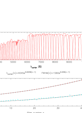
Figure 1: The transmission curves of the medium-band filters + U band used by the LZT (top graph) and the central wavelengths $\lambda_{\mathrm{center}}$ (crosses) and $FWHM$ of the filters multiplied by 10 (bottom graph).

2.2 Stars

Table 2: Star counts and $B-V$ colors predicted by the Bahcall-Soneira model of the Galaxy (Bahcall, 1986) for a limiting magnitude $R\leq 23$. The color noise is set to 0.1 mag. The spheroid giant branch is that of M13.

	Total	Disk	Spheroid
Star counts	3371	1445	1926
Mean $(B-V)$	1.07	1.46	0.76
Star fraction		43%	57%
Giant fraction	12%	0.4%	21%
$(B-V)$ bin
0.1-0.2	3.3	0.2	3.1
0.2-0.3	31.6	0.7	30.8
0.3-0.4	135.7	2.6	133.0
0.4-0.5	277.6	8.6	268.9
0.5-0.6	314.3	21.5	292.7
0.6-0.7	264.8	35.0	229.8
0.7-0.8	220.8	37.0	183.7
0.8-0.9	183.7	32.4	151.1
0.9-1.0	154.7	29.5	125.1
1.0-1.1	146.4	28.8	117.5
1.1-1.2	153.8	32.6	121.2
1.2-1.3	166.8	48.4	118.3
1.3-1.4	192.0	101.3	90.6
1.4-1.5	265.3	220.9	44.3
1.5-1.6	332.2	319.9	12.2
1.6-1.7	270.7	268.5	2.1
1.7-1.8	150.7	150.3	0.3
1.8-1.9	69.0	68.9	0.0
1.9-2.0	26.8	26.8	0.0
2.0-2.1	8.4	8.2	0.0
2.1-2.2	1.7	1.7	0.0

A phenomenological model producing the observed relative amounts of blue and red stars is sufficient for the mock catalog. We use the galaxy model of Bahcall & Soneira (Bahcall, 1986) (http://www.sns.ias.edu/$\sim$jnb/Html/galaxy.html html) to derive star counts and colors. Table 2 lists the star counts and colors predicted for a limiting magnitude of $R\leq 23$. The template spectra are collected from the star catalog of Pickles (1998), available at CDS (http://cdsweb.u-strasbg.fr/). This catalog contains 131 stellar spectra in the range 1150-10 620 Å, spanning all star temperatures (O to M), types (I to V), and metallicities (normal, rich, or poor). The template spectra are filtered using the transmission curves of Fig. 1. Figure 2 shows examples of template stellar spectra.

The simulation proceeds as follows. For each color bin in Table 2, we randomly draw the required number of templates (number of stars given in Table 2) from Pickles sub-sample of giant (or dwarf) templates. For instance, bin $0.5<B-V<0.6$ has 22 stars in the disk component (0.4%, that is zero stars are giant), and 293 stars in the spheroid component (21% are giant, that is 62 stars). Before stacking each drawn template to the final catalog, we add noise weighted by the expected LZT instrumental efficiency (see Sect. 2.5). The range of median signal-to-noise ratio in the continuum of the spectra which are generated is $6-100$.

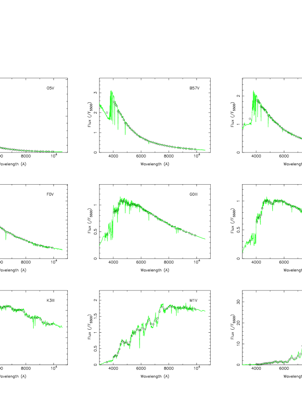
Figure 2: 9 templates of stellar spectra from the Pickles library (1998), containing 131 spectra. The high-resolution spectra ($R\simeq 2000$) are shown (grey line) along with the LZT-filtered flux ($\circ$). Spectral types are indicated.

The final mock catalog contains $\sim$ 3370 stellar templates, and faithfully reproduces the giant$/$dwarf fraction and the $B-V$ color distribution of Table 2.

2.3 Galaxies

2.3.1 Luminosity functions

Realistic simulations of galaxy morphology and redshift distributions are crucial but difficult because they require a prior knowledge of the morphological (or spectral) type-dependent LFs. The “intrinsic” LFs based on morphological type are only measured locally at $z\la 0.03$ (Binggeli et al., 1988; Marzke et al., 1994; Jerjen & Tammann, 1997; Marzke et al., 1998; Marinoni et al., 1999). Recent surveys to $z\sim 0.5-1$, in which galaxies are separated in 2 or 3 classes using colors or spectral measures indicate that the intrinsic LFs evolve with redshift (Lilly et al., 1995; Heyl et al., 1997; Lin et al., 1999; de Lapparent et al., 2002a), but the relation with the nearby LFs based on morphological type is not straightforward.

To simulate an approximate LZT galaxy catalog, we must choose a model for the intrinsic LFs in the redshift range of the LZT survey ($0\la z\la 1$). Because the LZT survey will be most sensitive in the red filters, Table 3 lists the galaxy LFs $\phi(M_{\mathrm{R}})$ of the existing red-band selected surveys which extend at or beyond $z\sim 0.5$. The deep blue-band selected survey by (Heyl et al., 1997) is therefore not considered. The LFs in Table 3 are defined by the Schechter parameterization (Schechter, 1976),

$$\phi(M)dM\leavevmode\nobreak\ = \leavevmode\nobreak\ 0.4\leavevmode\nobreak\ \ln{10}\leavevmode\nobreak\ \phi^{*}\leavevmode\nobreak\ 10^{-0.4(M^{*}-M)(\alpha+1)}dM$$ (1)

$$\leavevmode\nobreak\ \leavevmode\nobreak\ \leavevmode\nobreak\ \leavevmode\nobreak\ \leavevmode\nobreak\ \leavevmode\nobreak\ \leavevmode\nobreak\ \leavevmode\nobreak\ \leavevmode\nobreak\ \leavevmode\nobreak\ \times\left[-10^{0.4(M^{*}-M)}\right],$$

where $M$ is the absolute magnitude, and $\phi^{*}$, $M^{*}$, and $\alpha$ are the Schechter parameters. All parameters in Table 3 correspond to the case of a flat Universe with $\Lambda=0$ and $H_{0}=100h$ km s^-1 Mpc^-1.

The LFs in Table 3 are binned into early and late-type galaxies, and the measured evolution in the Schechter parameters is indicated for the samples in which it is detected. For the CNOC2 survey (Lin et al., 1999), the first class is their denoted “Early+Intermediate” class, and the second class is their denoted “Late” class; these classes are obtained by least-square fit to the SEDs by Coleman et al. (1980). For the ESS (de Lapparent et al., 2002b), the spectral classification is obtained by a PCA calibrated on the Kennicutt sample of nearby galaxy spectra (Kennicutt, 1992). Lilly et al. (1995) divide the CFRS sample into a population redder than Sbc, defined as having rest-frame $[U-V]_{\mathrm{AB}}=1.38$ ($[U-V]_{\mathrm{AB}}\simeq[V-I]_{\mathrm{AB}}$ at $z\sim 0.5$, $V_{\mathrm{AB}}=V$, and $I_{\mathrm{AB}}=I+0.48$), and a population bluer than Sbc, defined as the remaining galaxies. In Table 3, the Schechter LF parameter $M^{*}$ is listed in the $R_{\mathrm{c}}$ Cousins band, used by the CNOC2 (Lin et al., 1999) and the ESS (de Lapparent et al., 2002a, b). For the CFRS (Lilly et al., 1995), we use the $M^{*}$ values derived by the authors in the B_AB band for the galaxies with $0.2\leq z\leq 0.5$, and we convert them into the $R_{\mathrm{c}}$ band using $B_{\mathrm{AB}}=B-0.17$ (Lilly et al., 1995), and assuming $B-R_{\mathrm{c}}=1.35$ for galaxies redder than Sbc, and $B-R_{\mathrm{c}}=0.85$ for galaxies bluer than Sbc (Fukugita et al., 1995). Note that we have also converted the CFRS $M^{*}$ and $\phi^{*}$ from Lilly et al. (1995) from $H_{0}=50$ km s^-1 Mpc^-1 used by the authors, to $H_{0}=100h$ km s^-1 Mpc^-1 used here.

For comparison with a red-band selected survey at low redshift ($0\leq z\leq 0.2$), we also quote in Table 3 the LCRS survey (Bromley et al., 1998). The $r_{\mathrm{Gunn}}$ magnitudes are converted into $R_{\mathrm{c}}$ using $r_{\mathrm{Gunn}}-R_{\mathrm{c}}=0.36$ (Fukugita et al., 1995). For this survey, the spectral classification is obtained by a PCA, but it is not calibrated on spectra of known morphology. The grouping of galaxies into early and late-types must thus be done arbitrarily. In Table 3, we show the LFs obtained by grouping galaxies in clan $1+2+3+4$ into the early-types, and those in clans $5+6$ as the late-types. The corresponding listed Schechter parameters $M^{*}_{R}$ and $\alpha$ for the early and late-type galaxies are obtained by averaging the Schechter parameters over the considered clans. We calculate the corresponding amplitudes $\phi^{*}$ for the 2 average LFs by adjusting their integral in the absolute magnitude interval $-23\leq M_{R}\leq-16.5$ to the sum of the observed numbers of galaxies in the considered classes; a total survey area of 462 deg² is used (Shectman et al., 1996). The systematic bias against low surface-brightness galaxies which is present in the LCRS spectroscopic survey, tends to exclude late-type galaxies. This explains the relatively low $\phi^{*}(z\simeq 0)$ for the late-type galaxies in the LCRS as compared to the other surveys (by a factor of 3 to 5). This effect is might also be present in the LCRS early-type class (defined as clans $1+2+3+4$), and could explain the $\sim 50$% lower $\phi^{*}$ compared to that for the deeper surveys (ESS and CFRS).

Table 3: Parameters of the Schechter luminosity functions measured by various red-band galaxy surveys with $0<z<0.5$ (see text and Eq. 1).

Survey name	Galaxy Type	$N_{\mathrm{gal}}$	$M^{*}_{R_{\mathrm{c}}}-5\log h$	$\alpha$	$\phi^{*}$a	Evolution
and limits
CNOC2b
$0.1\la z\la 0.6$	Earlier than Sbc	1128	$-20.61\,\pm\,0.11$	$-0.44\,\pm\,0.10$	$0.023$	$M^{*}_{R}(z)\simeq M^{*}_{R}(z=0.3)^{\mathrm{c}}$
						$-0.7(z-0.3)$
$R_{\mathrm{c}}\leq 21.5$	Later than Sbc	1012	$-20.11\,\pm\,0.18$	$-1.34\,\pm\,0.12$	$0.006$	$\phi^{*}(z)\simeq\phi^{*}(z=0)^{\mathrm{d}}(1+3.17z)$
ESSe
$0.1\la z\la 0.5$	E+S0+Sa+Sb	436	$-20.49\,\pm\,0.11$	$-0.31\leavevmode\nobreak\ \,\pm\,0.14$	$0.031$
$R_{\mathrm{c}}\leq 20.5$	Sc+Sm/Im	181	$-19.84\,\pm\,0.24$	$-1.63\leavevmode\nobreak\ \,\pm\,0.22$	$0.006$	$\phi^{*}(z)\simeq\phi^{*}(z=0.15)^{\mathrm{d}}[1+3.5(z-0.15)]$
CFRSf
$0.2\la z\la 1.0$	Redder than Sbc	99	$-20.12\,\pm\,0.25$	$0.00\leavevmode\nobreak\ \leavevmode\nobreak\ \leavevmode\nobreak\ \leavevmode\nobreak\ \leavevmode\nobreak\ \leavevmode\nobreak\ \leavevmode\nobreak\ \leavevmode\nobreak\$	$0.030$
$I\leq 22.5$	Bluer than Sbc	110	$-20.01\,\pm\,0.25$	$-1.34\leavevmode\nobreak\ \leavevmode\nobreak\ \leavevmode\nobreak\ \leavevmode\nobreak\ \leavevmode\nobreak\ \leavevmode\nobreak\ \leavevmode\nobreak\ \leavevmode\nobreak\ \leavevmode\nobreak\ \leavevmode\nobreak\ \leavevmode\nobreak\$	$0.010$	1-mag brightening in $M^{*}_{R}$
						modelled here as $M^{*}_{R}(z)\simeq$
						$M^{*}_{R}(z=0.3)^{\mathrm{c}}-2(1-e^{0.3-z})$
LCRSg
$0\la z\la 0.2$	clans $1+2+3+4$	16146	$-20.42\,\pm\,0.02$	$-0.13\,\pm\,0.05$	$0.018$
$r_{\mathrm{Gunn}}\leq 17.7$	clans $5+6$	2132	$-20.38\,\pm\,0.08$	$-1.58\,\pm\,0.07$	$0.002$
LCRSg
$0\la z\la 0.2$	clans $1+2+3$	12936	$-20.50\,\pm\,0.03$	$0.03\,\pm\,0.05$	$0.012$
$r_{\mathrm{Gunn}}\leq 17.7$	clans $4+5+6$	5342	$-20.32\,\pm\,0.06$	$-1.27\,\pm\,0.05$	$0.006$
1-deg2 mock LZT
$0.2\la z\la 1.2$	early-type	$\sim$17300	$-20.42\leavevmode\nobreak\ \leavevmode\nobreak\ \leavevmode\nobreak\ \leavevmode\nobreak\ \leavevmode\nobreak\ \leavevmode\nobreak\ \leavevmode\nobreak\ \leavevmode\nobreak\ \leavevmode\nobreak\ \leavevmode\nobreak\ \leavevmode\nobreak\$	$-0.16\leavevmode\nobreak\ \leavevmode\nobreak\ \leavevmode\nobreak\ \leavevmode\nobreak\ \leavevmode\nobreak\ \leavevmode\nobreak\ \leavevmode\nobreak\ \leavevmode\nobreak\ \leavevmode\nobreak\ \leavevmode\nobreak\ \leavevmode\nobreak\$	0.03
$R_{\mathrm{c}}\leq 23.0$	late-type	$\sim$12700	$-20.18\leavevmode\nobreak\ \leavevmode\nobreak\ \leavevmode\nobreak\ \leavevmode\nobreak\ \leavevmode\nobreak\ \leavevmode\nobreak\ \leavevmode\nobreak\ \leavevmode\nobreak\ \leavevmode\nobreak\ \leavevmode\nobreak\ \leavevmode\nobreak\$	$-1.19\leavevmode\nobreak\ \leavevmode\nobreak\ \leavevmode\nobreak\ \leavevmode\nobreak\ \leavevmode\nobreak\ \leavevmode\nobreak\ \leavevmode\nobreak\ \leavevmode\nobreak\ \leavevmode\nobreak\ \leavevmode\nobreak\ \leavevmode\nobreak\$	0.01	$M^{*}_{R}(z)\simeq M^{*}_{R}(z=0.5)^{\mathrm{c}}$
						$-2(1-e^{0.5-z})$

Notes:
^a $\phi^{*}$ is in units of $h^{3}$ Mpc^-3. The quoted uncertainties in $\phi^{*}$ are typically of order of $0.005$. This is a lower limit if one takes into account the fluctuations caused by the large-scale clustering inside a given survey. For surveys which detect evolution in $\phi^{*}$, this Col. lists the value $\phi^{*}(z=0)$
^b Lin et al. (1999); the LFs are measured in the interval $-23\leq M_{\mathrm{R}}\leq-17$
^c value given in Col. $M^{*}_{R}-5\log h$
^d value given in Col. $\phi^{*}$
^e de Lapparent et al. (2002a, b); the LFs are measured in the interval $-23\leq M_{\mathrm{R}}\leq-16$
^f Lilly et al. (1996); the LFs are measured in the interval $-23.8\leq M_{B}(AB)\leq-19$ for red galaxies, and $-23\leq M_{B}(AB)\leq-19.5$ for blue galaxies
^g Bromley et al. (1998); the LFs are measured in the interval $-23\leq M_{\mathrm{R}}\leq-16.5$

We also show in Table 3, the LFs obtained for a different grouping of the LCRS clans: early-type are galaxies in clans $1+2+3$, and late-type are galaxies in clans $4+5+6$. The resulting variations in the Schechter luminosity functions illustrates the sensitivity of the intrinsic LFs to the scheme used for galaxy classification. The systematically low $\phi^{*}$ for both galaxy classes in either groupings ($1+2+3$ and $4+5+6$, $1+2+3+4$ and $5+6$) as compared to the deeper surveys CNOC2, ESS, and CFRS (see Table 3), further suggests that the LCRS suffers from selection effects causing an under-sampling of the galaxy populations.

The LFs for early and late-type galaxies at $z\ga 0.5$ listed in Table 3 show reasonable agreement among the various samples. The dominant source of variation in the LFs for each galaxy type are caused by the differences in the definitions of the spectral classes among the samples. This is reflected in the varying ratio of early to late-type galaxies among the surveys (see Col. $N_{\mathrm{gal}}$ in Table 3). Kochanek et al. (2000) recently showed that the mixing of the morphological classes which is often present in spectral classification can cause systematic biases in the parameters of the LFs. The varying selection effects from survey to survey (such as the mentioned bias in the LCRS against low-surface brightness objects) also contribute to the differences in the LFs.

The deep surveys quoted in Table 3 detect evolution of the LFs with redshift (Lilly et al., 1995; Lin et al., 1999; de Lapparent et al., 2002a). Understanding the details of this evolution is still a matter of debate. Here, we list some scenarii proposed in the corresponding articles. In the Lilly et al. (1995) survey, the red galaxies show no or little density or luminosity evolution in the range $0\la z\la 1$, whereas the blue galaxies show a luminosity evolution of at least 1 magnitude in that redshift range. The CNOC2 analysis separates the luminosity evolution from the density evolution. Early and intermediate-type galaxies show a small luminosity evolution in the range $0.1\la z\la 0.7$ ($\Delta M^{*}\simeq 0.5$), whereas late-type galaxies show a clear density evolution with almost no luminosity evolution in the same redshift range. Finally, for the ESS, an evolution in $\phi^{*}$ for the late-type galaxies is detected. These various evolutions are listed in Table 3, in the Col. labeled “Evolution”.

Figure 3: Galaxy redshift distribution in 40 deg² of the sky to $17\leq R_{\mathrm{c}}\leq 23$ in an Einstein-de Sitter Universe, according to the LFs measured from the CNOC2 data (Lin et al., 1999) and listed in Table 3. The non-evolving and evolving distributions for the early+intermediate galaxies are shown as a thin dashed line, resp. thick dashed line, and for the late-type galaxies, as a thin dotted line, resp. thick dotted line. The non-evolving and evolving total distributions are shown as thin solid line, resp. thick solid line.

Figure 4: Galaxy redshift distribution in 40 deg² of the sky to $17\leq R_{\mathrm{c}}\leq 23$ in an Einstein-de Sitter Universe, according to the LFs measured from the ESS data (de Lapparent et al., 2002a, b) and listed in Table 3. The non-evolving distribution for the early-type galaxies is shown as a thin dashed line, and for the late-type galaxies, as a thin dotted line. The evolving distribution for the late-type galaxies is shown as a thick dotted line, and is modeled as $\phi^{*}(z)\simeq\phi^{*}(z=0.15)[1+3.5(z-0.15)]$. The non-evolving and evolving total distributions are shown as thin solid line, resp. thick solid line.

Figure 5: Galaxy redshift distribution in 40 deg² of the sky to $17\leq R_{\mathrm{c}}\leq 23$ in an Einstein-de Sitter Universe, according to the LFs measured from the CFRS data (Lilly et al., 1995) and listed in Table 3. The non-evolving distribution for the red galaxies is shown as a thin dashed line, and for the blue galaxies, as a thin dotted line. The evolving distribution for the blue galaxies is shown as a thick dotted line, and is modeled as $M^{*}_{R}(z)\simeq M^{*}_{R}(z=0.3)-2(1-e^{0.3-z})$ (see Table 3). The non-evolving and evolving total distributions are shown as thin solid line, resp. thick solid line.

Figures 3, 4, and 5 show for each survey displayed in Table 3 the redshift distributions calculated for the listed Schechter parameters: without evolution (thin dashed line for early-type galaxies, and thin dotted line for late-type galaxies), and with evolution when it applies (thick dashed line for early-type galaxies, thick dotted line for late-type galaxies). These predicted redshift distributions are calculated in the case of a flat Universe with $\Lambda=0$ and $H_{0}=100h$ km s^-1 Mpc^-1, over the $40$ deg² planned area for the LZT survey, and are extrapolated to the limiting magnitude of the LZT survey, namely $R_{\mathrm{c}}\leq 23.0$. In Fig. 5, we model the observed evolution of the CFRS blue LF with a brightening in $M^{*}_{R}$, defined by the additive term $m(z)=-2[1-\exp-(z-0.3)]$; this yields $m=0.0$ for $z=0.3$, $m=-1.0$ for $z=0.6$, $m=-1.9$ for $z=1.0$, and $m=-2.7$ for $z=1.5$. For comparison, the redshift distributions for the early and late-type LFs for the LCRS divided in clans $1+2+3$ and $4+5+6$ are shown in Fig. 6 (no evolution is considered).

Figure 6: Galaxy redshift distribution in 40 deg² of the sky to $17\leq R_{\mathrm{c}}\leq 23$ in an Einstein-de Sitter Universe, according to the LFs measured from the LCRS data (Bromley et al., 1998) and listed in Table 3. The distribution for the galaxies in clans $1+2+3$ is shown as a thin dashed line, and as a thin dotted line for galaxies in clans $4+5+6$. The thin solid line shows the total distribution.

In Figs. 3, 4, 5, the systematic differences between the evolving early-type/red and late-type/blue galaxy redshift distributions show common properties. The peak for the late-type distribution is at smaller redshift than that for the early-type distribution because of the combination of fainter $M^{*}$ and steeper slope $\alpha$ for the first class of objects. This effect is preserved when evolution of the early-type and/or late-type population are introduced, despite the fact that all evolution scenarii quoted in Table 3 tend to shift the peaks of the redshift distributions to higher redshift. The interesting result derived from the comparison of Figs. 3, 4, 5, is that the 3 parameterizations of the LF evolution lead to resembling galaxy redshift distributions in the range $0\la z\la 1$ at the depth of the LZT survey ($R_{\mathrm{c}}\leq 23.0$): the redshift and amplitude at the peak, as well as the high redshift fall-off of the redshift distributions are similar. In contrast, the LCRS produces a systematically low redshift distribution at this depth, with a peak at $\sim 600$ galaxies, whereas the no-evolution curves for the deeper surveys shown in Figs. 3, 4, 5, all peak in the range $\sim 900-1200$ galaxies; as already mentioned, this may arise from selection effects in the LCRS.

We therefore choose to adopt for all mock catalogues considered here the following LF Schechter parameters: $M^{*}_{R}=-20.42$, $\alpha=-0.16$, $\phi^{*}=0.03$ for early-type galaxies; $M^{*}_{R}=-20.18$, $\alpha=-1.19$, $\phi^{*}=0.01$ for late-type galaxies (also listed in Table 3). These chosen $\alpha$ for the early-type galaxies, and the $M^{*}_{R}$ and $\phi^{*}$ for both galaxy types are within the range of values measured for the 3 $R$-selected surveys in Table 3: the CNOC2, the ESS, and the LCRS. The slope $\alpha=-1.19$ for the late-type galaxies is flatter than the flattest measured slope (from the LCRS, clans $4+5+6$), in order to limit the number of galaxies to be included in the mock LZT catalogues, and thus the computing time for the PCA; this value is however only $1.25\sigma$ flatter than the slope of the LF for the CNOC2 late-type galaxies. Having a steeper slope for the late-type galaxies would have a weak impact on the results presented here. Note that the chosen values of $\phi^{*}$ for the early and late-type LFs are obtained by using an early-type to late-type $\phi^{*}$ ratio of 3 (as in the CFRS) and by normalizing the total number of galaxies per deg² with $R_{\mathrm{c}}\leq 23$ to the observations: numerous studies give galaxy counts in the $R$ band, and we use a typical value of $\sim 30,000$ galaxies/deg² (Roche et al., 1996; Metcalfe et al., 2001).

Figure 7: Predicted redshift distribution for the future LZT survey in 40 deg² of the sky to $17\leq R_{\mathrm{c}}\leq 23$ in an Einstein-de Sitter Universe. The redshift distributions for the non-evolving early-type, late-type galaxies are shown as a thin dashed line, resp. thin dotted line. The corresponding Schechter parameters are $M^{*}_{R}=-20.42$, $\alpha=-0.16$, $\phi^{*}=0.03$ for the early-type galaxies, and $M^{*}_{R}(z\leq 0.5)=-20.18$, $\alpha=-1.19$, $\phi^{*}=0.01$, for the late-type galaxies. The expected distribution for the evolving late-type galaxies, modeled by an $M^{*}_{R}$ brightening define by $M^{*}_{R}(z\geq 0.5)\simeq M^{*}_{R}(z=0.5)-2(1-e^{0.5-z})$ is shown as a thick dotted line. The thin, resp. thick continuous lines show the sums of the curves for the non-evolving early-type galaxies and the non-evolving, resp. evolving late-type galaxies. The evolving sum is subsequently used for generating the mock LZT catalogues.

Because the LZT survey will have a depth comparable with that of the CFRS, we adopt an evolution of the LF resembling that for the CFRS, but which better matches the evolution at $z>1$ (as shown in Fig. 7, a non negligeable fraction of galaxies, $27$%, will have $z\geq 1$ in the LZT survey). Although the evolution of the galaxy LFs is poorly known beyond $z=1$, photometric redshifts applied to the Hubble Deep Field do provide a general trend for the evolution of the “total” LF: a steepening of the slope $\alpha$ from $-1.3$ ($z\sim 0.5$) to $-2$ ($z\sim 3$), and a one magnitude brightening of $M^{*}_{B}$ between $z\sim 1$ and $z\sim 3$ (Sawicki et al., 1997; Takeuchi et al., 2000). We therefore conservatively assume no evolution of both the early and late-type galaxy LFs in the range $0\leq z\leq 0.5$, and add a brightening term $m(z)=-2[1-\exp-(z-0.5)]$ to $M^{*}_{R}$ for the LZT blue galaxies with $z\geq 0.5$. The brightening term $m(z)$ gradually changes $M^{*}_{R}$ by $m=-0.83$ at $z=1$, $m=-1.0$ at $z=1.19$, $m=-1.26$ at $z=-1.5$, $m=-1.55$ at $z=2$, and $m=-1.8$ at $z=3$; it asymptotically reaches its ceiling of $m=-2$ at $z\geq 3$. The corresponding redshift distribution for the evolving late-type galaxies in the modeled LZT survey is given in Fig. 7 (thick dotted line); it is combined with the non-evolving early-type redshift distribution (thin dashed line) to derive the sum of the 2 populations in the evolving model (thick continuous line). This summed redshift distribution is subsequently adopted for the LZT mock surveys analyzed here. For comparison, the corresponding non-evolving late-type galaxies distribution (thin dotted line) and non-evolving total distribution (thick continuous line) are also shown in Fig. 7.

Figure 8: Galaxy template spectra from GISSEL (Bruzual & Charlot, 1993). In each frame, the Initial Mass Function (IMF) and metallicity of the spectra vary from top to bottom as follows: Salpeter IMF, with 20% solar, 40% solar, and solar metallicity; Scalo IMF, with 20% solar, 40% solar, and solar metallicity.

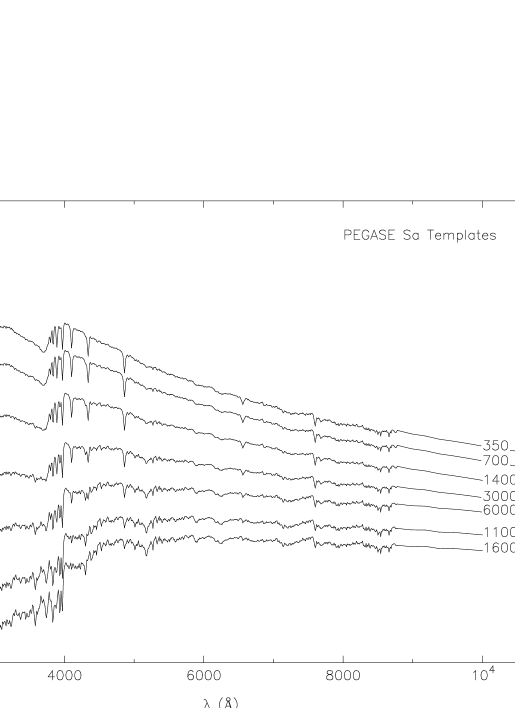
Figure 9: Sa13 galaxy template spectra from PEGASE (Fioc & Rocca-Volmerange, 1997). The age of the spectra are given in million years. The metallicity is adjusted to have a solar value for the 13-Gyr-old spectrum.

Over the planned area of $40$ deg² for the LZT survey, over $\sim 1,000,000$ galaxies are expected. Because the PCA is computer-time consuming, we limit the size of the LZT mock catalogues used in the following analyses to 1 deg². These calatogue therefore include $\sim 30,000$ galaxies, and the number of galaxies in each class are those listed in Table 3.

2.3.2 Galaxy spectral energy distributions

The galaxy templates are extracted from stellar synthesis libraries. Figure 8 shows 24 templates of E/S0, Sa/Sb, Sc/Sd, and Sm/Im galaxies for 3 metallicities and 2 Initial Mass Functions (IMF) kindly provided by S. Charlot, and calculated from the version GISSEL95 of the GISSEL evolutionary code (Bruzual & Charlot, 1993). For early-type galaxies, higher metallicities flatten the slope of the continua. Changing the IMFs induces no effect on the templates (Fig. 8, frame a). For late-type galaxies, the Salpeter IMF (Salpeter, 1955) tends to produce bluer objects than the Scalo IMF (Miller & Scalo, 1979), and the metallicity effect is small (Fig. 8, frames b to d). The Sa/Sb templates using a Salpeter IMF are very similar to the Sc/Sd templates using a Scalo IMF, and at the resolution of the LZT survey, they are nearly identical.

Alternatively, the PEGASE package (Fioc & Rocca-Volmerange, 1997) allows us to generate a set of solar metallicity spectra with different ages, different stellar formation rates (SFR) and different IMF taken from Rana & Basu (1992). Details can be found in Fioc & Rocca-Volmerange (1997). Included in the PEGASE package is an atlas of templates of eight galaxy types. For the various spectral types (E, S0, Sa, etc…), the atlas provides 65 templates from ages of 1 Myr to 16 Gyr; each age sequence is normalized so that the 13-Gyr templates fit present day SEDs of observed galaxies with solar metallicity.

Even if true spectra cover a large range of metallicities and ages, the resolution $R\simeq 40$ of the LZT survey does not allow us to distinguish between a PEGASE young Sa galaxy template and PEGASE old Sb, Sc, Sd or Im galaxy template. Therefore, we include in the mock LZT catalog only templates showing significant differences and instead of using the ages given by PEGASE as true indicators of the evolution of galaxies with redshift, we use them as indicators of the morphological sequence. Hence, for elliptical galaxy SEDs, we use the 23 templates of the PEGASE atlas called E13 and older than 1 Gyr (the templates have a short SFR, followed by passive evolution). For spiral galaxy SEDs, we use the 31 templates of the PEGASE atlas called Sa13, older than 350 Myr (we use a constant SFR for spiral galaxies). Figure 9 shows several Sa13 templates from the PEGASE library, shown at various ages. As already mentioned, the 13-Gyr-old template is fitted to a local Sa galaxy spectra with solar metallicity. We interpret the ages sequence given by PEGASE Sa13 templates as follows: late-type galaxies (Sc, Sd, Im) are modeled by young Sa13 galaxy templates (with ages $<3$ Gyr, 15 templates), and early-type galaxies (Sa, Sb) by old Sa13 galaxy templates (with ages $\geq 3$ Gyr, 16 templates).

There are notable differences between PEGASE and GISSEL elliptical galaxies in the UV, whereas spiral templates look alike in both models. We also emphasize that both GISSEL and PEGASE packages rely on the stellar library of Pickles which is noticeably deficient in AGB stars SEDs. AGB stars are still poorly known but represent a non-negligeable part of the total integrated flux of galaxies.

The mock LZT galaxy catalogues are built using the (evolving) redshift distributions in Fig. 7. Early-type galaxies are randomly extracted from the 12 GISSEL E/S0/Sa/Sb templates, the 23 PEGASE E13 templates, and the 16 Sa13 templates older than 3 Gyr. Late-type galaxies are randomly extracted from the 12 GISSEL Sc/Sd/Sm/Im templates, and the 15 PEGASE Sa13 templates younger than 3 Gyr. The number of early and late-type galaxies are those plotted in Fig. 7 as non-evolving early-type and evolving late-type redshift distributions for the LZT survey (see also Table 3).

2.3.3 Emission-line galaxies

We do not model the emission lines in the galaxy SEDs, because in the medium-band filters used by the LZT, only the brightest emission lines will be detected. At first order, an emission line will be detected only if

$$\frac{W_{\mathrm{line}}}{W_{\mathrm{filter}}}\geq\frac{Threshold}{S/N},$$ (2)

where $W_{\mathrm{line}}$ is the line equivalent width, $W_{\mathrm{filter}}$ is the filter bandwidth, $Threshold$ is the detection threshold in units of standard deviation, and $S/N$ is the signal-to-noise ratio. For $Threshold=1$, $S/N=3$, and a typical $W_{\mathrm{filter}}=150$Å, the emission line must have $W_{\mathrm{line}}\geq$ 50Å. Only QSOs and Seyfert galaxies reach this level of emission.

We emphasize that the analysis of the QSO sub-sample included in the LZT mock catalog (see next Sect.) demonstrates that strong emission lines contribute to improving the object classification and the redshift determination which are obtained by the PCA. As seen in Fig. 14 and described in Sect. 3.1 below, the PCA sequence of QSOs is clearly separated from the blue part of the stellar sequence, and this is caused by the strong emission lines present in the QSO SEDs.

Although Seyfert galaxies only represent a small fraction ($5\%$) of the galaxy populations at low redshift (Reichert, 1992), the fraction of galaxies with strong emission lines may be larger at $z\ga 0.5$. However, we consider that it is not necessary to include them in the mock LZT catalogues, as they have similar SEDs to QSOs, and would therefore make a negligeable change to the PCA eigenbasis. Seyfert galaxies and other galaxies with strong emission lines would deviate from the locus of normal galaxies in the PCA, and would thus be easily identified; their redshift would be measured with similar accuracy as for the QSOs (see Sect. 5). They could also be directly identified from their SEDs using a break-finding algorithm (Cabanac et al., 1998), or a cross-correlation analysis (as shown by preliminary tests performed by R. Cabanac).

2.4 Quasi-stellar objects

The third kind of objects included in the simulations are the quasi-stellar objects (QSO). We use the preliminary results of the on-going 2dF QSO Survey (Boyle et al., 2000). The 2dF QSO survey has been optically selected in the $U$, $B_{J}$ and $R$ bands from UKST photographic plates. The $B_{J}$ QSO LF is found to follow a pure luminosity evolution (Boyle et al., 2000) which can be modeled by

$$\phi(L_{B},z)dL = \frac{\phi_{B}^{*}dL}{\displaystyle\left[\frac{L_{B}}{L_{B}^{*}(z)}\right]^{3.6}+\left[\frac{L_{B}}{L_{B}^{*}(z)}\right]^{1.8}}$$ (3)

$${\rm with\leavevmode\nobreak\ \leavevmode\nobreak\ \leavevmode\nobreak\ \leavevmode\nobreak\ \leavevmode\nobreak\ \leavevmode\nobreak\ \leavevmode\nobreak\ \leavevmode\nobreak\ \leavevmode\nobreak\ \leavevmode\nobreak\ \leavevmode\nobreak\ \leavevmode\nobreak\ \leavevmode\nobreak\ \leavevmode\nobreak\ }$$

$$\log\left[\frac{L_{B}^{*}(z)}{L_{B}^{*}(0)}\right] = 1.4z-0.27z^{2},$$ (4)

$${\rm or\,\,equivalently}$$

$$M_{B}^{*}(z) = M_{B}^{*}(0)-2.5\,(1.4z-0.27z^{2}),$$ (5)

We assume the same analytical description for the $R$ QSO LF, and choose to adopt for the simulations $M_{R}^{*}\simeq-21$ and $\phi_{R}^{*}=10^{-6}$ Mpc^-3 mag^-1, a $\sim 35$% larger value than calculated from the $B_{J}$ 2dF survey (Boyle et al., 2000). Equation 3 can be rewritten in terms of absolute magnitude $M_{R}$:

$$\phi(M_{R},z)dM_{R} = \frac{0.4ln(10)\Phi_{R}^{*}dM_{R}}{X^{3.6-1}+X^{1.8-1}},$$

$$X = 10^{0.4[M^{*}_{R}(0)-M_{R}]-1.4z+0.27z^{2}}.$$ (6)

We assume that Eq. 6 is a reasonable prediction of the LZT QSO sample and we extrapolate the QSO LF to the LZT apparent magnitude limit of $R_{\mathrm{c}}\leq 23$. We also set a bright cut off at $R_{\mathrm{c}}=15$. The resulting redshift distribution in the interval $0\leq z\leq 4$ is shown in Fig. 10.

Figure 10: Redshift distribution for QSOs with $15\leq R_{\mathrm{c}}\leq 23$ in an Einstein-de Sitter Universe, using the 2dF QSO survey LF (Boyle et al., 2000).

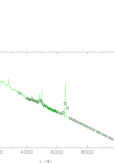
Figure 11: Composite QSO spectrum at $z=0$ (Francis et al., 1991). The wavelengths of the centers of the LZT filters are overlaid ($\circ$). At red wavelengths, the spectrum is extrapolated by a power-law from 6000 to 10⁴ Å, to which is added a synthetic H_α line. In the UV, the spectrum is completed with observations from HST (Zheng et al., 1997).

Figure 10 shows a composite QSO template derived from the LBQS sample (Francis et al., 1991), and a sample of 101 QSOs observed in the UV using HST (Zheng et al., 1997). Because the QSO template provided by Francis et al. is bounded at 6000 Å, and the LZT filters extend out to 10⁴ Å, we approximate the missing continuum by a power-law in the range 6000-10 000 Å. In the blue, the composite spectrum is bounded at 800 Å. In order to define the U and blue LZT magnitudes for all QSOs with $z\leq 4$, we extrapolate the spectrum to 300 Å at a constant flux. Note that because of Lyman $\alpha$ absorption, the continuum of the spectrum is poorly defined at wavelengths bluer than $\sim 1200$ Å (see Vanden Berk et al., 2001); this choice only affects QSOs with $z\geq 2.75$, among which, only those with weak emission lines would be “lost” in the star sample. We also add a synthetic $H_{\alpha}$ emission line whose intensity is related to the intensity of the $H_{\beta}$ emission line already present in the composite spectrum, according to the typical $H_{\alpha}/H_{\beta}$ line ratio of $\sim 4$, obtained in models of broad line regions (Osterbrock, 1989). A new composite spectra has been made available by the SDSS consortium (Vanden Berk et al., 2001) while the present article was in the refereeing process. Because both the emission lines and the continua of the 2 composite spectra are remarkably similar, we did not update our simulations to include the SDSS composite spectrum: the wide spectral range of the SDSS spectrum would make no improvement to our analysis, as the range covered by the 2dF composite spectrum used here is sufficient to describe the full wavelength interval of the LZT filters for QSOs with $0\la z\la 4$.

The integrated QSO number count per deg² is extrapolated from the differential number counts in the 2dF QSO survey (Boyle et al., 2000). To a limiting apparent magnitude of $R\leq 23$, the integrated count of QSOs per square degree is $\sim 130$. The mock LZT catalogues are generated for 1 deg², hence each simulation is obtained by randomly drawing $130$ QSO templates with the same redshift distribution as in Fig. 10, and subsequently adding noise according to the LZT efficiency (see the next Sect.). The range of signal-to-noise ratio in the continuum of the synthetic QSO spectra is $3-100$.

Because the number of QSOs is relatively small in our mock catalogues we decided to use only the composite SED of Francis without slope variations. Nevertheless, it is likely that the slopes of the continuum of real QSO SEDs vary around the mean slope of the composite SED of Francis. The effect of such a variation on the PCA would be to spread the locus of QSOs from a line to a surface; the area of this surface would be related to the standard deviation in the variation of the slope. This variation could degrade the identification of QSOs, because the flatter the slopes, the higher the similarities between QSOs and emission-line galaxies. On the other hand, the measured redshift accuracies (Sect. 5) should not be affected by this simplification.

2.5 Noise

Photon noise and detector read-out noise are added to the SED of each type of object according to the response curve $T(\lambda)$ of the Large Zenith Telescope (LZT), defined as the product of the detector sensitivity curve $CCD(\lambda)$ by the transmission curve of the telescope/instrument optics $O(\lambda)$, and the sky transmission $I(\lambda)$:

$$T(\lambda)=I(\lambda)\;O(\lambda)\;CCD(\lambda);$$ (7)

For an object with intrinsic flux $F_{0}(\lambda)$, the final flux $F(\lambda)$ obtained after “observing” the object with the LZT telescope+instrument+detector and correcting it using an absolute flux calibration is

$$F(\lambda)=F_{0}(\lambda)\left[1+\frac{gauss}{S/N(\lambda)}\right]$$ (8)

with

$$S/N(\lambda) = \frac{\sqrt{\frac{T(\lambda)\;N_{\mathrm{night}}}{g(\lambda)}}\;F_{0}(\lambda)}{\sqrt{F_{0}(\lambda)+A_{\mathrm{src}}\;sky(\lambda)+\frac{A_{\mathrm{src}}\;RON^{2}\;g(\lambda)}{A_{\mathrm{pix}}\;T(\lambda)\;N_{\mathrm{night}}}}},$$ (9)

$$g(\lambda) = \frac{10^{20}\;hc}{\lambda_{c}\;\Delta\lambda\;\Delta t\;A_{\mathrm{mirror}}}.$$ (10)

$gauss$ is a gaussian random generator, with a null mean and a root-mean-square dispersion of 1, $S/N(\lambda)$ is the “observed” signal-to-noise ratio in the spectrum $F(\lambda)$; $sky(\lambda)$ is a composite sky spectrum, using Kitt Peak night sky spectrum (Massey & Foltz, 2000), Mauna Kea KECK LRIS OH emission lines atlas (http://www2.keck.hawaii.edu), and GEMINI near IR modeled continuum (http://www.us-gemini.noao.edu). Figure 12 shows the composite high-resolution sky spectrum and its medium-band counterpart using the LZT filters. In Eq. 9, $A_{\mathrm{src}}$ is the area of the observed object in arcsec² on the detector, $A_{\mathrm{pix}}=0.245$ arcsec² is the area of one CCD pixel, $RON=11$ e^- is the CCD readout noise. The function $g(\lambda)$ in Eq. 10 is the flux expressed in Joule/second/meter³ corresponding to one photon having the central wavelength $\lambda_{c}$ of the LZT filter considered (see Fig. 1), arriving on the detector per exposure time $\Delta t$ and per wavelength interval $\Delta\lambda$ (of the considered filter), given the area of the LZT mirror $A_{\mathrm{mirror}}=28.3$ m² (wavelengths are expressed in meters, time in seconds); $hc=1.992^{-25}$ J$\cdot$m is the product of the Planck constant by the speed of light. Because the LZT is operated in drift-scan mode, the exposure time is fixed to $\Delta t=65$ sec. The exposure time is effectively increased by observing a given region of the survey in a given filter during several nights $N_{\mathrm{night}}$ (see Eq. 9).

Figure 12: Composite sky spectrum using Kitt Peak night sky spectrum (Massey & Foltz, 2000), Mauna Kea KECK LRIS OH emission lines atlas (http://www2.keck.hawaii.edu), and GEMINI near IR modeled continuum (http://www.us-gemini.noao.edu). The filled diamonds are the LZT U+medium-band filter fluxes used for noise computations.

Figure 13: Signal-to-noise distributions ($S/N[\lambda]$) of 3 stellar spectra with types O5V, G0V, and M6V, with median $S/N$ of 44, 14, and 122 resp.. The lowest $S/N$ is set to $3.35$ (dotted line): its corresponds to the signal-to-noise ratio of a punctual source extended over 5 contiguous pixels, with a detection threshold of 1.5 per pixel.

The number of optical surfaces in the telescope/instrument combination is 11: the mirror (80% reflectivity), and 4 lenses plus the CCD window (98% transmission is assumed for each of the 10 surfaces). For simplicity the transmission is supposed to be achromatic. The LZT total efficiency curve $T(\lambda)$ has a bell-shape between 3000Å  and 10000Å, with a flat maximum transmission of 0.65 running from 5000Å  to 8000Å. Figure 13 shows the $S/N(\lambda)$ calculated using Eq. 9 for an O5V star, a G0V star and an M6V star, with their lowest signal-to-noise ratio set to 3.35: this corresponds to the overall signal-to-noise ratio obtained from 5 contiguous pixels having each a signal-to-noise ratio of 1.5. Note that we choose such a low detection level per pixel in order to test the PCA. Given the LZT median seeing of 0.9 arcsec FWHM (Full-Width-Half-Maximum), we do not expect stars to be less extended than 5 pixels, as it corresponds to the area of a disk of 1.2-arcsec diameter projected onto CCD pixels with an area $A_{\mathrm{pix}}=0.245$ arcsec². We thus adopt the limiting signal-to-noise ratio of $3.35$ as our detection threshold for the LZT mock catalog. For galaxies at $z\simeq 0.5$, a typical FWHM of 3 arcsec (see Sect. 4.1) yields an area of 28.8 pixels, and a detection threshold of $S/N=1.5$ per pixel yields an overall $S/N\sim 8$.

We also define the overall signal-to-noise of each spectrum as the median value of $S/N(\lambda)$ over the 41 LZT filters. For the spectra in fig. 13, these median $S/N$ are 44 (O5V), 14 (G0V), and 122 (M6V). Figure 13 therefore illustrates that very blue or very red spectra must have a high median $S/N$ to be detected over the entire range of the LZT filters. To simplify the analysis and interpretation, the SEDs of all classes/types of objects in a given mock catalog are set to the same median signal-to-noise ratio. Mock catalogues are generated such that only objects with a lower filter above the threshold limit of $S/N(\lambda)=3.35$ and median signal-to-noise ratio equal to a given value are included: any object having at least one filter with a $S/N(\lambda)<3.35$ is therefore not included in the catalog. Catalogues with median signal-to-noise ratios of $100,\,20,\,10$, and $6$ are used for the analysis reported here. In the following Sects., the labels $S/N$ always refer to the median signal-to-noise ratio of the spectra in the mock catalogue considered. As shown in Fig. 13, we emphasize that at a median $S/N$ ratio of 100, the bluest objects will have a signal-to-noise ratio of $\sim 10$ in their reddest filters, whereas the reddest objects will have a signal-to-noise ratio of $\sim 3$ in their bluest filters; for flat-spectrum objects, the range of signal-to-noise ratio described by the spectra will be narrower.

3 Methodology

3.1 Principal Component Analysis

For a detailed description of the PCA, the reader is referred to the books of Murtagh & Heck (1987) or Kendall (1972), and to the seminal paper of Connolly et al. (1995b). In this section we outline the results of PCA and develop the classification method.
Following Connolly et al. (1995b), consider a set $f$ of $N$ vectors $f_{i}$ of $M$ elements $f_{\lambda i},\leavevmode\nobreak\ i\in\{1\ldots N\},\leavevmode\nobreak\ \lambda\in\{1\ldots M\}$, normalized to have unit scalar products $[f_{i}\cdot f_{i}]^{1/2}=1$. In our case, $M$ is the number of filters: $M=41$. The PCA derives a set of $min(N,M)$ orthogonal eigenvectors $e_{j}$ (that is $M=41$ eigenvectors in the present case, as $N\gg M$), using criteria of decreasing maximum variance of the spectra when projected onto the eigenvectors. Each vector $f_{i}$ can be written as a linear combination of $e_{j}$:

$$f_{\lambda i}=\sum_{j=1}^{M}y_{ij}e_{\lambda j},$$ (11)

where $y_{ij}$, denoted eigencomponent, is the weight of the $j$th eigenvector in the $i$th vector. The first eigenvector $e_{1}$ is the mean vector over the $f_{\lambda i}$. Each weight $y_{i1}$ measures how much $f_{\lambda i}$ is similar to the mean vector, i.e. gives its projection onto the mean vector; the second vector $e_{2}$ lies in the direction of highest variance orthogonal to $e_{1}$ etc.

The main advantage of the PCA is that when the vectors $f_{i}$ are correlated (as it is the case for astronomical SEDs), most of the discriminatory power of the linear combination (Eq. 11) is carried by the first few eigenvectors, and the high-order eigenvectors carry mostly the noise of the spectra. The PCA therefore provides a powerful filter for the set $f$ (see Galaz and de Lapparent, 1998). For illustration, Table 4 shows the eigenvalues $\gamma_{j}$ of a PCA performed on one mock LZT catalog described in Sect. 2. As shown by Connolly et al. (1995b), each eigenvalue $\gamma_{j}$ is the contribution of the corresponding eigenvector $e_{j}$ to the variance of the set $f$, and therefore describes the relative power of each eigenvector in the dataset (one can intuitively realize that if all vectors have similar directions, they can be described by a small number of components). The power $P_{j}$ carried by each eigenvector $e_{j}$ can be measured as

$$P_{j}=\frac{\gamma_{j}}{\sum_{j=1}^{M}\gamma_{j}}.$$ (12)

Table 4 therefore shows that the first 3 eigenvectors $e_{1}$, $e_{2}$, $e_{3}$ carry 87.6%, 9%, 2.2% resp. of the descriptive power; the sum of these 3 contributions yields 98.8%, and adding $e_{4}$ increases the summed contributions to 99.3%. This means that the first 3 vectors actually carry most of the information and, to a good approximation, the weights of the other eigenvectors may be neglected. This is the reason why only the first 3 or 4 eigencomponents are usually kept to describe a set of galaxies at $z=0$ (Ronen et al., 1999).

Table 4: Eigenvalues $\gamma_{j}$ of a typical PCA derived eigenbasis $e$ from a LZT mock catalog which contains a mix of 3368 stars, 11600 galaxies and 170 QSO SEDs with $S/N=100$, as described in Sect. 2. The first 3 eigenvalues contain 98.8% of the descriptive power.

$e_{j}$	$\gamma_{j}$	$e_{j}$	$\gamma_{j}$	$e_{j}$	$\gamma_{j}$
$e_{1}$	13230.44	$e_{15}$	1.198	$e_{29}$	0.076
$e_{2}$	1355.23	$e_{16}$	1.004	$e_{30}$	0.070
$e_{3}$	340.38	$e_{17}$	0.972	$e_{31}$	0.057
$e_{4}$	71.54	$e_{18}$	0.775	$e_{32}$	0.055
$e_{5}$	35.57	$e_{19}$	0.703	$e_{33}$	0.051
$e_{6}$	25.90	$e_{20}$	0.563	$e_{34}$	0.007
$e_{7}$	16.70	$e_{21}$	0.465	$e_{35}$	0.010
$e_{8}$	6.434	$e_{22}$	0.426	$e_{36}$	0.014
$e_{9}$	4.450	$e_{23}$	0.369	$e_{37}$	0.042
$e_{10}$	3.045	$e_{24}$	0.282	$e_{38}$	0.021
$e_{11}$	2.917	$e_{25}$	0.199	$e_{39}$	0.026
$e_{12}$	2.041	$e_{26}$	0.190	$e_{40}$	0.031
$e_{13}$	1.862	$e_{27}$	0.136	$e_{41}$	0.028
$e_{14}$	1.589	$e_{28}$	0.120

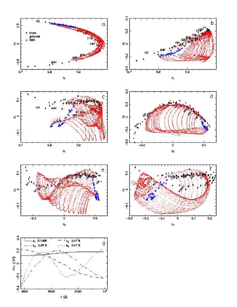
Figure 14: PCA eigencomponents $y_{2}$ versus $y_{1}$ a), $y_{3}$ versus $y_{1}$ b), $y_{4}$ versus $y_{1}$ c), $y_{3}$ versus $y_{2}$ d), $y_{4}$ versus $y_{2}$ e), $y_{4}$ versus $y_{3}$ f), and a plot of the first 4 eigenvectors g) for a catalog containing 131 stars ($\ast$), 7800 galaxies ($\cdot$) and 80 QSOs ($\circ$) at a median signal-to-noise ratio of $S/N=100$ (see Sect. 2). The 3 classes of objects occupy different regions of the graphs. Galaxies and QSOs show clear redshift sequences. The loci of the various stellar types are indicated in each graph.

Our case is more complex because we have to analyze a catalog containing different classes of objects, which in addition span different redshift intervals, hence showing a wide variety of spectral energy distributions. We therefore need to use all significant information. Several tests were performed, with PCAs having 4, 5, 6, 7, 8, 9, 10 and 20 eigencomponents. Fewer than 5 components is largely insufficient to describe the LZT mock samples (see Sect. 6.1). One must reach 9 components to restore the full details of the LZT mock samples. We therefore choose to perform the analysis of the LZT mock catalogues with a 10-eigencomponent PCA, as the remaining power after the 10th component just reaches below 0.1% (see Table 4 and Eq. 12). With 10 eigencomponents, Eq. 11 then becomes

$$f_{\lambda i}\simeq\sum_{j=1}^{10}y_{ij}e_{\lambda j}.$$ (13)

Figure 14 plots the first 4 weights or PCA eigencomponents $y_{1}$, $y_{2}$, $y_{3}$, and $y_{4}$ resulting from a PCA on the same mock catalog that used to obtain Table 4. The last graph shows the corresponding first 4 eigenvectors; the corresponding relative powers which they carry are indicated in the graph. Stars (stars) galaxies (dotted lines) and QSOs (open circles) occupy well-defined regions of the 4-D space described by the first 4 eigenvectors $e_{1}$, $e_{2}$, $e_{3}$, and $e_{4}$ (see frames b & d). As shown by Connolly et al. (1995b) and Galaz & de Lapparent (1998), using the first 3 eigencomponents, the stellar spectral sequence (shown with asterisks) describes an arc, with later type being at lower values of $y_{2}$. The stellar spectral types of selected stars are indicated in each graph. O, B, and A stars have positive values of $y_{2}$, whereas M stars have negative values of $y_{2}$. The other spectral types fill the sequence. The galaxies (plotted as dots) describe a 2-D surface, starting from the stellar sequence at low redshift, and extending away from it along the paths generated by a redshift step of $0.01$. The higher redshift considered for the galaxies is $\sim 2$. The QSOs (open circles) describe a linear sequence defined by their redshift ($1\leq z\leq 4$). The QSO sequence is distinct from the stellar sequence at low redshift, and merges with it at $z\sim 3$ (see Sect. 4.2); at this redshift, a QSO cannot be distinguished from an F star.

Therefore, the PCA not only provides a spectral classification within each class of object (stars, galaxies, QSOs) but also allows a classification scheme by which the 3 classes of objects can be distinguished. The definition of the different spectral types for each class of object can be done by parameterization of the 1-D or 2-D surfaces they describe. This is developed in Sect. 3.3.

3.2 The spectral classification

Because the PCA is a non-parametric approach, the eigenvectors derived for one catalog are specific and maybe inappropriate for another catalog. In order to use the PCA for spectral classification, one must relate the internal correlations outlined by the PCA with the physical properties of the objects. The canonical but subjective method to achieve this purpose, is to create realistic mock catalogues of templates and apply the PCA to them. Previous works by Connolly et al. (1995a); Connolly & Szalay (1999), Galaz & de Lapparent (1998) and Ronen et al. (1999) establish the efficiency of the PCA to produce an internal classification scheme related to physical properties of galaxies. For instance, Galaz & de Lapparent (1998) use the first 3 eigencomponents $y_{i1}$, $y_{i2}$, and $y_{i3}$ as Cartesian coordinates of a 3-D space, and convert them into the 2 angles defining the corresponding spherical coordinates which are in turn used for the classification: one parameter is related to the color of the objects, i.e. the slope of the continua, and the other is an index of the intensity of the emission lines. Ronen et al. (1999) show by using stellar synthesis galaxy template spectra that one can track down some properties such as the age or the metallicity. The weakness of the method of Ronen et al. is that when the stellar synthesis models reproduce the observed spectra but are physically wrong, the derived physical properties are erroneous. A successful approach should include a direct calibration of the PCA on observed spectra with known types, ages, and metallicities (Galaz & de Lapparent, 1998).

As pointed out by Connolly et al. (1995b), the PCA eigenvectors and corresponding eigencomponents are determined by the relative numbers of the different types of objects. Connolly et al. (1995b) introduce a morphological type normalization to account for this relative proportion of objects when catalogues with unrealistic proportions are used. Here, we prefer the direct approach of using realistic mock catalogues (see Sect. 2) which will be directly comparable to the LZT catalog.

The PCA applied to the mock LZT catalogues is used here to extract the relevant information for classifying objects and measuring their redshifts (for galaxies and QSOs). We choose a simple approach. Once the principal eigencomponents of the mock catalog are measured, we select the first 10 eigenvectors and define a 10-dimensional eigenbasis, in which each class of object occupies a given locus, defined by it spectral type among its class, and its redshift for galaxies and QSOs. As the paths followed by the galaxies and QSO are monotonic functions of redshift, the PCA provides a template-independent method for measuring redshifts. Except for the redshift/spectral-type degeneracies discussed in Sect. 6.1, similar types of objects at similar redshifts (for galaxies and QSOs) tend to be nearby in the space defined by the 10-dimensional eigenbasis, thus providing a unique parameterization of a given SED. In the following, we describe how the object classes and types are defined and how the redshifts are measured.

3.3 Definition and measurement of object/spectral types

We define object classes (star, galaxy, QSO) and types (O to M for stars, E to Irr for galaxies) by assigning to each template a number $T$. For stars, the 131 Pickles templates spanning the range of stellar types O to M and luminosities I to V are ordered from blue to red and are assigned types $T\in\{1,2,...,131\}$. Galaxies are also ordered from blue to red as follows: the 12 GISSEL late-type templates (see Sect. 2.3.2); the 27 PEGASE late-type templates; the 12 GISSEL early-type templates; the 27 PEGASE early-type templates; these 78 spectra are assigned types $T\in\{132,133,...,209\}$. QSOs are all assigned $T=210$, as only one type of spectrum was used.

Given the SED $o_{\lambda}$ of an object. The projected components on the eigenbasis $o^{p}_{j}$ are simple scalar products:

$$o^{p}_{j}=o_{\lambda}\cdot e_{\lambda j}=\sum^{41}_{\lambda=1}o_{\lambda}e_{\lambda j},$$ (14)

and the weighted distance $d$ from the object to any other object $i$ of the 10-D space is

$$d=\left[\sum^{10}_{j=1}\gamma_{j}^{1/2}(o^{p}_{j}-y_{ij})^{2}\right]^{1/2}.$$ (15)

where $y_{ij}$ are the eigencomponents defined in Eq. 11 and 13, $e_{j}$ are the corresponding eigenvectors of the PCA performed on the mock catalog. Weighting the eigencomponents with their eigenvalues $\gamma_{j}$ is used to account for the increase in the noise from $y_{i1}$ to $y_{i10}$. The object type $T_{\mathrm{object}}$ is simply defined as the arithmetic mean of the types $T_{y_{i}}$ of the $\eta$ nearest neighbors:

$$T_{\mathrm{object}}=\overline{T}=\frac{1}{\eta}\sum^{\eta}_{i=1}T_{y_{i}}.$$ (16)

As a test, we calculate for our mock catalogues of 2993 galaxies with median $S/N=20$ and $10$, and for those with 2095 galaxies with median $S/N=6$, the type $T_{\mathrm{object}}$ given by Eq. 16 for $\eta=1,2,3,4,5,$ and $10$. The resulting errors in the object classes and types are listed in Table 5: Cols. $\pm 5,\pm 10,\pm 15$ and $>15$, give the number of galaxies for which $T_{\mathrm{object}}$ differs from the true type $T$ by 5, 10, 15, and more than 15 type units; Cols. star and QSO give the number of galaxies misclassified as star, or QSO. Table 5 demonstrates that in all cases, the most accurate results are obtained for $\eta=1$, i.e. the nearest neighbor is always the best choice. The efficiency of the classification is further described in Sect. 4.

Note that in the nearest neighbor analysis used here, the effect of the input $S/N$ onto the eigencomponents $y_{i}$ is not accounted for. Table 5 suggests that the effect on the classification would be negligeable (as almost no errors occur even for large values of $\eta$). The effect on the type and redshift determination would be larger, and we refer the reader to Sect. 6.1 for a more general discussion.

Table 5: Error in the determination of the types for 2993 galaxies at median $S/N=20$, 10, and 2095 galaxies at median $S/N=6$, for different values of $\eta$ (see text for details).

Median $S/N=20$
$\eta$	type error #				class error #
	$\pm 5$	$\pm 10$	$\pm 15$	$>15$	star	QSO
1	2796	14	20	133	0	0
2	2769	23	22	149	0	0
3	2756	24	33	150	0	0
4	2746	38	22	157	0	0
5	2726	56	27	154	0	0
10	2703	50	50	160	0	0
Median $S/N=10$
$\eta$	type error #				class error #
	$\pm 5$	$\pm 10$	$\pm 15$	$>15$	star	QSO
1	2509	76	32	374	0	0
2	2469	75	43	404	0	0
3	2455	86	71	379	0	0
4	2433	125	40	393	0	0
5	2418	130	65	378	0	0
10	2400	128	76	387	0	0
Median $S/N=6$
$\eta$	type error #				class error #
	$\pm 5$	$\pm 10$	$\pm 15$	$>15$	star	QSO
1	1594	84	85	332	0	0
2	1577	114	73	331	0	0
3	1587	105	88	315	0	0
4	1578	136	61	320	0	0
5	1590	126	62	317	0	0
10	1584	143	52	316	0	0

3.4 Measurement of redshifts

Because we apply the PCA to the observed SEDs, it is possible to measure redshifts directly with a technique similar to the classification method (Sect. 3.2). In the 10-D space defined by the first 10 eigenvectors, galaxies and quasars follow redshift sequences. We define the redshift $z_{o}$ of an unknown object as the average redshift $\bar{z}$ of the $\eta$ nearest neighbors from the mock catalog which lie inside a radius $r_{\eta}$ and have type $T_{\mathrm{object}}\pm 5$:

$$z_{o}=\bar{z}=\frac{1}{\eta}\sum^{\eta}_{i=1}z^{T_{\mathrm{object}}}_{y_{i}};$$ (17)

$r_{\eta}$ is defined by $\eta$ and has the same unit as $d$ (Eq. 15), and therefore, as the eigencomponents $y_{i}$ (see Eq. 11 and Fig. 14). The value of $r_{\eta}$ is usually small: for $\eta=10$, we estimate $r_{\eta}\la 0.05$ for the 3 classes of object. If more than one class is present among the $\eta$ neighbors, i.e. if the object falls in a locus containing a mix of various classes, the class is not robustly defined and the average redshift is given for all classes inside $r_{\eta}$. Our mock catalog is such that for 98% of the galaxies, the redshift accuracy is not strongly dependent on $\eta$ for $\eta<5$, and for 90% of the QSOs, $\eta=1$, i.e., the nearest neighbor always provides a more accurate redshift than the average over a group of objects (the remaining 2% galaxies and 10% QSOs are affected by degeneracies in redshifts, which are described in Sect. 6.1).

4 Star/galaxy/QSO separation

In this section we examine quantitatively how the separation of stars, galaxies and QSOs can be performed using the PCA, and how the object profile can contribute to the analysis.

4.1 Extended versus unresolved objects

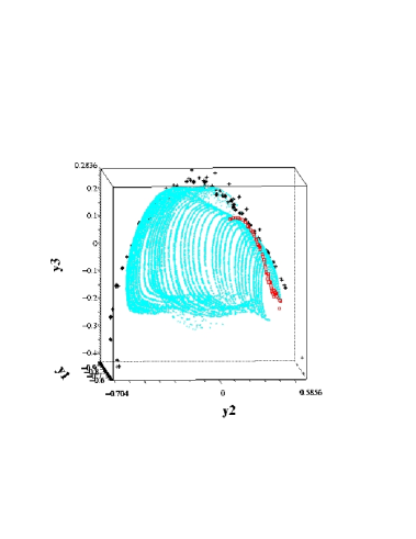
Figure 15: PCA projections $y_{1}$, $y_{2}$, and $y_{3}$ for a mock LZT catalog of 33,486 objects (3370 stars [+], 29,986 galaxies [$\cdot$] and 130 QSOs [squares]). The SEDs have a median $S/N\simeq 100$.

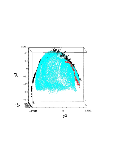
Figure 16: Same as in Fig. 15 for a median $S/N\simeq 20$.

In an Einstein-de Sitter universe, the angular size $\theta$ of an object with physical size $D$ is

$$\theta(z)=(DH_{0}/2c)(1+z)^{2}[(1+z)-(1+z)^{1/2}]^{-1}$$ (18)

where $c=300,000$ km s^-1, and $H_{0}$ is the Hubble constant. Following Sandage, Kron & Longair Sandage et al. (1995), a typical disk galaxy has an effective diameter of $D=10$ kpc, which results in an angular size $\theta(z=0.25)=4.09\arcsec$; this value assumes a mean surface brightness in Johnson $V$ band $\mu_{V}=23.5$ mag$\cdot$arcsec^-2, and an exponential disk profile (see Table 6.2, p. 283, in Sandage, Kron & Longair, 1995). For $\mu_{V}=25.1$ mag$\cdot$arcsec^-2, the angular size $\theta(z=0.5)=2.8\arcsec$. Hence, most of bright galaxies at $z\la 0.5$ are expected to be more extended than the PSF of the LZT ($\sim 1-2\arcsec$), and potential confusion between star and galaxy SEDs is not expected to occur beyond redshift $0.2$. At redshifts higher than $0.2$, the PCA is indeed robust to segregate stars from galaxies due to the red-shifting of the galaxy SEDs. Only compact galaxies at low redshifts ($z\la 0.2$) might be intrinsically difficult to distinguish from stars in the medium-band system of the LZT. So far there is no evidence for a dominating population of compact galaxies at these redshifts. Moreover, the fraction of galaxies in the predicted LZT redshift distribution of Fig. 7 lying at $z\leq 0.2$ is $\sim 10$%, a non-negligeable but minor component of the full sample.

4.2 PCA classification efficiency

Table 6: Error in the classification of $\sim$ 3000 stars, $\sim$ 3000 galaxies, and $\sim$ 1000 QSOs for different values of median signal-to-noise ratio $S/N$ (see text for details).

. Median $S/N$ Input ^a Classification # ^b class # Stars Galaxies QSOs Stars 3181 3181 0 0 100 Galaxies 2993 0 2993 0 QSOs 984 0 0 984 Stars 2843 2833 10 0 20 Galaxies 2993 0 2993 0 QSOs 984 0 0 984 Stars 2092 2092 0 0 10 Galaxies 2993 0 2993 0 QSOs 984 6 0 978 Stars 1956 1923 0 33 6 Galaxies 2095 0 2095 0 QSOs 741 42 9 690

^a Input number of objects in each class
^b Output number of stars, galaxies, and QSOs derived by the 10-component PCA

One key parameter in determining the efficiency of the PCA classification is the signal-to-noise ratio in the spectra. Figure 15 shows a 3D plot of the first 3 eigencomponents of the PCA performed on mock catalogues containing 33,486 objects (3370 stars, 29,986 galaxies and 130 QSOs) and a median signal-to-noise ratio $S/N\simeq 100$ (see Sect. 2.5). This catalog represents a sub-area of 1 deg² of the future LZT survey, and the PCA method is that described in Sect. 3.2, based on the first 10 eigencomponents. In Fig. 16, the mock catalog of Fig. 15 is degraded to a median signal-to-noise ratio $S/N\simeq 20$. In both Figs., stars, galaxies and QSOs occupy different loci in the 3D-space, therefore allowing us to separate objectively the 3 classes of objects, and illustrating how the PCA is robust to noise.

Table 6 compiles the efficiency of the classification as a function of signal-to-noise ratio for a small mock catalog described in Sect. 5 below. Following the previous Sect., we assume that the 1347 galaxies at $z\la 0.5$ are extended, and thus can be separated from stars using morphological criteria. The remaining 1646 galaxies at $z\ga 0.5$ are separated from stars and QSOs using Eq. 16. For a median $S/N=100$, the object classification is perfect, and although it slowly degrades as the signal-to-noise ratio decreases, the performance of the classification are weakly dependent on the signal-to-noise ratio.

Table 6 shows that QSO SEDs tend to be misclassified as stellar SEDs ($6\%$ of QSOs at a median signal-to-noise ratio of 6). There is no degeneracy between blue stars (O, B or white dwarfs) and low-redshift QSOs, because blue stars have no emission lines; QSOs are thus clearly segregated. In the range $2.5<z<3$, QSO and F/G stellar SEDs are similar. For $z\ga 3.5$, QSO signatures are unique again and misclassification is rare. Unfortunately, the range $2.5<z<3$ corresponds to the peak of the expected QSO distribution (see Sect. 2.4). This explains why such a large fraction of QSOs are misclassified as stars for median $S/N=6$. This outlines a weakness of this classification method, the solution of which probably lies in a slightly different approach which we discuss in Sect. 6.

Table 7: Error in the determination of the type for stars and galaxies, for different values of median signal-to-noise ratio $S/N$. Stars have a total of 131 types, and galaxies have 78 types (see text for details).

Median $S/N$	Object class	type error # a
		$\pm 5$	$\pm 10$	$\pm 15$	$>15$
100	Stars	3177	3	0	1
	Galaxies	2916	0	4	25
20	Stars	2617	163	33	30
	Galaxies	2796	14	20	133
10	Stars	1658	290	73	71
	Galaxies	2509	76	32	374
6	Stars	1560	317	38	41
	Galaxies	1594	85	84	332

^a Number of objects classified within $\pm 5$, $\pm 10$, $\pm 15$ and more than $\pm 15$ of their input types

4.3 PCA type identifications

Table 7 allows us to evaluate the accuracies in the type identifications for the 2 classes of objects having types (stars and galaxies). The accuracies are measured by the difference between the real type and the PCA-measured type, as in Table 5. For galaxies, an error of $\pm 10$ on the type leads to a catastrophic error in redshift in $1/3$ of the cases, and an error of $\pm 15$ or more leads systematically to a catastrophic error in redshift. Table 7 shows the results for the 4 median signal-to-noise ratios $S/N=100,20,10,6$.
At a median $S/N=100$, the PCA is able to discriminate O,B,A,F,G,K,M star types and most luminosity and metallicity classes. At a median $S/N=20$, metallicity differences within each stellar type are no longer discriminated, and the luminosity class I, II, III, IV, V is often mismatched. At a median $S/N=10$ and lower, only major continuum differences allow one to discriminate between different stellar types. Table 7 shows that even at $S/N=6$, the PCA is able to discriminate types for half of the objects within each class.

5 Redshift measurement accuracy

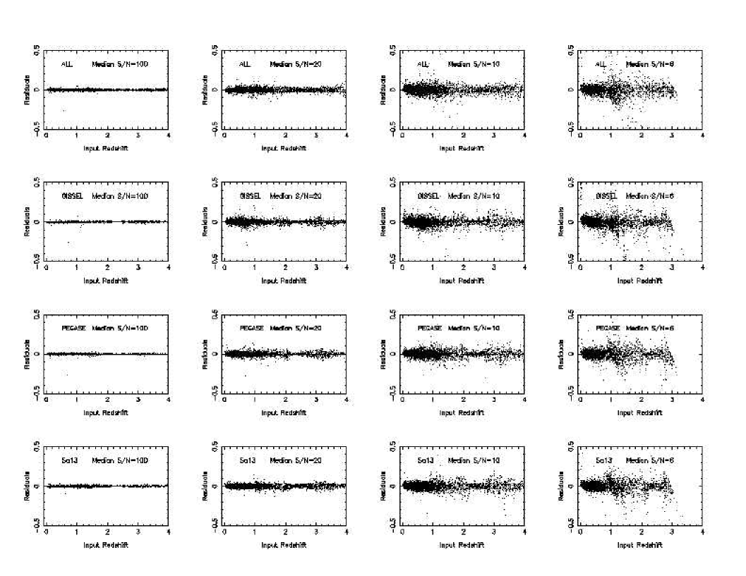
Figure 17: Redshift residuals versus input redshift extracted from a $\chi^{2}$ reduction of the first 10 PCA eigencomponents. In each frame, spectra in sub-mock catalogues are projected onto realistic mock simulations with a median signal-to-noise ratio of $S/N=100$. ¿From top to bottom, in addition to $\sim 3000$ stars and $\sim 1000$ QSOs, the sub-mock calatogues include $\sim 3000$ galaxy SEDs drawn respectively from only the 78 galaxy templates of PEGASE+GISSEL (ALL), from only the 24 galaxy templates of GISSEL, from only the 54 PEGASE templates (PEGASE), and from only the 31 PEGASE Sa13 templates (Sa13). In all frames, only QSOs have redshifts $z>2$. The corresponding standard deviations are listed in Tables 8 to 12.

Table 8: Residuals in the redshift measurements for sub-mock simulations including $\sim 3000$ stars, $\sim 1000$ QSOs, and $\sim 3000$ galaxy SEDs with a median signal-to-noise ratio of 100 (see also Fig. 17).

Median $S/N=100$
$z$	ALL			GISSEL			PEGASE			PEGASE Sa13
	#	$\bar{z}$	$\sigma_{\mathrm{Res.}}$	#	$\bar{z}$	$\sigma_{\mathrm{Res.}}$	#	$\bar{z}$	$\sigma_{\mathrm{Res.}}$	#	$\bar{z}$	$\sigma_{\mathrm{Res.}}$
0.1	243	-0.0002	0.006	244	-0.0003	0.004	243	-0.0002	0.004	251	0.0004	0.004
0.2	334	-0.0001	0.004	336	-0.0001	0.003	325	0.0001	0.003	329	0.0000	0.003
0.3	354	-0.0004	0.014	358	-0.0003	0.004	358	-0.0003	0.004	359	-0.0003	0.003
0.4	357	0.0001	0.005	354	-0.0004	0.014	326	-0.0004	0.004	351	0.0003	0.005
0.5	319	-0.0001	0.005	318	-0.0005	0.004	288	-0.0001	0.004	325	0.0002	0.006
0.6	293	-0.0005	0.004	291	-0.0001	0.004	258	0.0001	0.004	288	0.0001	0.004
0.7	254	0.0004	0.004	251	-0.0003	0.003	221	0.0004	0.005	254	-0.0001	0.004
0.8	219	-0.0006	0.005	225	0.0001	0.003	177	-0.0001	0.006	224	0.0001	0.004
0.9	181	0.0002	0.005	181	0.0003	0.004	147	0.0008	0.005	178	-0.0002	0.006
1.0	148	0.0002	0.008	146	0.0010	0.010	114	-0.0012	0.005	150	-0.0005	0.006
1.1	111	-0.0004	0.007	114	-0.0005	0.005	90	-0.0003	0.006	110	0.0007	0.006
1.2	90	-0.0002	0.007	88	-0.0010	0.004	66	-0.0005	0.009	90	0.0003	0.006
1.3	68	-0.0009	0.010	68	-0.0007	0.004	52	-0.0012	0.008	64	0.0003	0.008
1.4	51	0.0006	0.009	49	-0.0009	0.004	47	-0.0001	0.009	54	-0.0045	0.006
1.5	48	-0.0010	0.011	50	0.0001	0.003	41	0.0000	0.008	47	0.0009	0.007
1.6	40	0.0009	0.010	40	0.0003	0.005	39	-0.0025	0.009	40	0.0002	0.008
1.7	39	0.0027	0.007	39	-0.0011	0.006	35	-0.0026	0.007	39	0.0004	0.007
1.8	35	-0.0003	0.008	35	-0.0003	0.007	31	-0.0010	0.006	35	-0.0031	0.007
1.9	34	-0.0000	0.007	29	-0.0017	0.005	31	-0.0010	0.006	32	0.0003	0.007
2.0	40	-0.0005	0.006	45	0.0024	0.007	43	0.0005	0.007	42	-0.0010	0.007
2.5	44	0.0005	0.004	48	-0.0002	0.006	50	-0.0008	0.006	46	0.0009	0.005
3.0	40	-0.0002	0.006	39	0.0021	0.007	39	-0.0031	0.007	42	-0.0005	0.005
3.5	31	-0.0010	0.005	27	-0.0004	0.005	28	0.0025	0.008	32	0.0025	0.006

Notes:
at $z<2$, $z$ is the redshift of the galaxies binned by intervals of 0.1
at $z\geq 2$, $z$ is the redshift of the QSOs binned by intervals of 0.5
# is the number of galaxies or QSOs in the redshift bin considered
$\bar{z}$ is the average residual in the redshift
$\sigma_{\mathrm{Res.}}$ is the r.m.s. dispersion in the redshifts errors defined as $\Delta z=|z_{\mathrm{PCA}}-z_{\mathrm{input}}|$
ALL corresponds to sub-mock catalogues with galaxies drawn from all galaxy templates
GISSEL corresponds to sub-mock catalogues with galaxies drawn from GISSEL templates only
PEGASE corresponds to sub-mock catalogues with galaxies drawn from PEGASE templates only
PEGASE Sa13 corresponds to sub-mock catalogues with galaxies drawn from PEGASE Sa13 templates only

Table 9: Same as in Table 8 for a median signal-to-noise ratio of 20 (see also Fig. 17).

Median $S/N=20$
$z$	ALL			GISSEL			PEGASE			PEGASE Sa13
	#	$\bar{z}$	$\sigma_{Res.}$	#	$\bar{z}$	$\sigma_{Res.}$	#	$\bar{z}$	$\sigma_{Res.}$	#	$\bar{z}$	$\sigma_{Res.}$
0.1	242	-0.0012	0.014	242	-0.0002	0.016	245	0.0003	0.015	248	-0.0008	0.012
0.2	330	-0.0010	0.013	335	0.0008	0.015	333	-0.0010	0.012	330	0.0005	0.012
0.3	360	-0.0002	0.013	354	-0.0003	0.015	351	-0.0000	0.013	357	-0.0009	0.013
0.4	353	0.0009	0.016	355	-0.0027	0.030	357	-0.0017	0.021	354	0.0010	0.014
0.5	319	0.0023	0.019	317	-0.0019	0.024	322	-0.0009	0.018	320	0.0010	0.016
0.6	295	0.0015	0.017	296	0.0007	0.028	293	-0.0002	0.016	290	-0.0004	0.014
0.7	251	0.0004	0.019	251	-0.0015	0.021	253	-0.0001	0.018	257	-0.0005	0.013
0.8	219	-0.0021	0.021	220	-0.0013	0.021	217	0.0001	0.019	218	0.0003	0.015
0.9	181	0.0020	0.020	179	0.0027	0.021	183	-0.0020	0.019	180	-0.0009	0.018
1.0	147	0.0023	0.024	155	-0.0004	0.021	149	0.0031	0.026	149	0.0008	0.026
1.1	116	0.0034	0.026	108	0.0064	0.039	112	-0.0016	0.022	114	-0.0008	0.025
1.2	86	-0.0008	0.025	91	0.0007	0.020	87	0.0001	0.026	88	-0.0035	0.026
1.3	66	0.0005	0.032	66	-0.0014	0.015	67	0.0032	0.021	66	0.0091	0.023
1.4	53	-0.0023	0.025	50	-0.0023	0.015	51	0.0046	0.018	52	-0.0027	0.019
1.5	48	0.0057	0.082	49	0.0006	0.015	48	-0.0019	0.025	49	-0.0027	0.032
1.6	40	-0.0052	0.032	39	0.0004	0.019	40	0.0003	0.023	40	-0.0067	0.020
1.7	39	0.0171	0.114	40	0.0053	0.041	40	0.0091	0.029	39	-0.0047	0.027
1.8	35	-0.0051	0.025	35	0.0017	0.032	35	-0.0049	0.027	35	-0.0034	0.031
1.9	33	-0.0021	0.023	34	0.0047	0.027	32	-0.0100	0.033	31	-0.0094	0.026
2.0	41	0.0034	0.022	40	0.0027	0.026	42	-0.0036	0.029	43	0.0023	0.030
2.5	46	-0.0030	0.013	44	0.0005	0.013	46	0.0011	0.016	47	0.0028	0.012
3.0	38	-0.0037	0.019	39	-0.0021	0.034	37	0.0016	0.029	42	0.0012	0.033
3.5	28	-0.0068	0.017	29	-0.0117	0.023	29	0.0100	0.020	29	0.0041	0.018

Table 10: Same as in Table 8 for a median signal-to-noise ratio of 10 (see also Fig. 17).

Median $S/N=10$
$z$	ALL			GISSEL			PEGASE			PEGASE Sa13
	#	$\bar{z}$	$\sigma_{Res.}$	#	$\bar{z}$	$\sigma_{Res.}$	#	$\bar{z}$	$\sigma_{Res.}$	#	$\bar{z}$	$\sigma_{Res.}$
0.1	243	-0.0006	0.026	245	0.0072	0.030	241	-0.0002	0.023	242	-0.0010	0.022
0.2	333	0.0019	0.028	327	0.0007	0.032	329	0.0013	0.020	333	-0.0010	0.023
0.3	356	-0.0030	0.027	360	-0.0008	0.034	360	0.0010	0.025	357	0.0015	0.025
0.4	358	-0.0025	0.032	353	-0.0089	0.039	357	-0.0011	0.030	347	-0.0016	0.034
0.5	320	-0.0038	0.033	325	-0.0078	0.039	317	-0.0023	0.029	323	0.0006	0.029
0.6	290	-0.0020	0.031	289	-0.0070	0.044	296	0.0025	0.034	296	0.0000	0.025
0.7	256	0.0022	0.039	250	-0.0053	0.036	250	0.0025	0.037	249	-0.0010	0.027
0.8	218	-0.0023	0.037	221	-0.0096	0.041	223	0.0004	0.032	227	-0.0043	0.031
0.9	179	-0.0016	0.043	179	-0.0090	0.050	178	0.0015	0.036	175	-0.0017	0.032
1.0	153	-0.0005	0.085	152	-0.0103	0.062	146	0.0002	0.04	151	0.0052	0.0436
1.1	108	-0.0041	0.068	113	-0.0119	0.045	115	0.0010	0.047	112	-0.0008	0.050
1.2	92	0.0184	0.102	86	0.0081	0.044	89	-0.0034	0.061	89	-0.0038	0.053
1.3	67	-0.0006	0.042	68	-0.0008	0.038	66	0.0063	0.042	66	0.0158	0.056
1.4	49	-0.0038	0.045	50	-0.0059	0.035	49	0.0005	0.046	50	0.0002	0.043
1.5	50	-0.0121	0.066	48	0.0030	0.059	51	0.0066	0.068	49	-0.0024	0.084
1.6	40	0.0385	0.165	40	-0.0007	0.107	39	0.0388	0.143	40	0.0028	0.041
1.7	39	0.0404	0.196	40	0.0199	0.108	40	0.0380	0.143	40	0.0142	0.105
1.8	35	0.0017	0.094	35	0.0083	0.044	35	-0.0080	0.052	35	-0.0046	0.056
1.9	27	0.0411	0.124	33	0.0112	0.056	31	-0.0010	0.053	33	-0.0061	0.078
2.0	47	0.0217	0.113	41	-0.0051	0.058	43	0.0116	0.057	41	-0.0012	0.060
2.5	44	-0.0032	0.032	46	0.0083	0.030	44	0.0023	0.025	46	0.0028	0.023
3.0	41	0.0002	0.031	41	-0.0078	0.074	39	-0.0115	0.068	42	-0.0155	0.094
3.5	28	0.0014	0.042	32	0.0059	0.056	32	0.0206	0.041	29	-0.0045	0.048

Table 11: Same as in Table 8 for a median signal-to-noise ratio of 6 (see also Fig. 17).

Median $S/N=6$
$z$	ALL			GISSEL			PEGASE			PEGASE Sa13
	#	$\bar{z}$	$\sigma_{Res.}$	#	$\bar{z}$	$\sigma_{Res.}$	#	$\bar{z}$	$\sigma_{Res.}$	#	$\bar{z}$	$\sigma_{Res.}$
0.1	216	0.0055	0.026	217	0.0126	0.031	217	0.0029	0.030	208	0.0026	0.028
0.2	269	0.0028	0.033	262	0.0065	0.039	261	-0.0007	0.032	266	0.0010	0.036
0.3	260	0.0010	0.037	267	0.0070	0.113	266	0.0013	0.033	270	-0.0002	0.030
0.4	222	-0.0007	0.099	223	0.0013	0.069	222	-0.0029	0.050	220	0.0039	0.051
0.5	175	0.0004	0.053	173	0.0014	0.067	177	0.0009	0.064	177	-0.0021	0.039
0.6	129	0.0018	0.065	131	-0.0027	0.082	128	0.0035	0.067	131	0.0048	0.045
0.7	90	-0.0008	0.052	89	0.0012	0.063	91	0.0043	0.042	86	0.0045	0.039
0.8	118	-0.0807	0.185	122	-0.0223	0.091	58	0.0038	0.045	60	0.0027	0.047
0.9	184	-0.1366	0.237	174	-0.0654	0.146	102	-0.0253	0.124	101	-0.0113	0.091
1.0	144	-0.0965	0.249	155	-0.0812	0.156	146	-0.0568	0.168	148	0.0007	0.092
1.1	116	-0.0639	0.235	107	-0.0132	0.089	112	-0.0248	0.122	113	-0.0036	0.098
1.2	87	0.0239	0.207	91	-0.0076	0.129	89	-0.0248	0.122	89	-0.0108	0.091
1.3	66	0.0209	0.244	63	0.0265	0.133	67	-0.0043	0.114	65	-0.0013	0.103
1.4	50	0.0617	0.233	50	-0.0102	0.093	51	-0.0042	0.148	52	0.0058	0.083
1.5	49	0.0577	0.266	52	0.0114	0.131	50	0.0117	0.111	49	-0.0024	0.111
1.6	41	0.1385	0.339	40	0.0030	0.110	39	0.0313	0.151	39	-0.0060	0.078
1.7	39	0.0411	0.248	39	-0.0152	0.123	40	0.0186	0.184	40	0.0388	0.140
1.8	35	0.1317	0.355	35	-0.0077	0.109	35	0.0211	0.081	35	-0.0220	0.122
1.9	34	0.1615	0.354	31	-0.0210	0.100	32	0.0062	0.089	34	-0.0141	0.082
2.0	39	0.0182	0.186	43	0.0056	0.081	42	0.0129	0.084	40	-0.0185	0.073
2.5	39	0.0377	0.154	47	-0.0117	0.074	45	-0.0276	0.087	48	-0.0137	0.070
3.0	35	0.0111	0.054	38	-0.0132	0.116	38	-0.0216	0.097	38	-0.0145	0.120

Table 12: Residuals in the galaxy redshift measurements binned by increasing redshift for the simulations including GISSEL templates only on a PCA including PEGASE templates only, for various median signal-to-noise ratios (see also Fig. 18).

$z$	Median $S/N=100$			Median $S/N=20$			Median $S/N=10$			Median $S/N=6$
	#	$\bar{z}$	$\sigma_{Res.}$	#	$\bar{z}$	$\sigma_{Res.}$	#	$\bar{z}$	$\sigma_{Res.}$
0.1	244	-0.0024	0.021	242	-0.0024	0.023	245	-0.0013	0.033	217	0.0066	0.041
0.2	336	-0.0012	0.022	335	-0.0031	0.023	327	-0.0068	0.034	262	-0.0107	0.056
0.3	358	-0.0022	0.028	354	-0.0038	0.033	360	-0.0112	0.040	267	-0.0160	0.076
0.4	354	-0.0128	0.044	355	-0.0125	0.046	353	-0.0249	0.050	223	-0.0313	0.059
0.5	318	-0.0206	0.049	317	-0.0172	0.049	325	-0.0263	0.051	173	-0.0392	0.056
0.6	247	-0.0183	0.047	286	-0.0252	0.050	289	-0.0329	0.055	131	-0.0508	0.062
0.7	184	-0.0459	0.048	251	-0.0426	0.046	251	-0.0468	0.055	89	-0.0557	0.101
0.8	157	-0.0581	0.057	220	-0.0557	0.049	221	-0.0834	0.124	122	-0.1634	0.220
0.9	124	-0.1432	0.220	161	-0.1066	0.176	179	-0.1298	0.204	174	-0.3560	0.284
1.0	86	-0.1900	0.254	110	-0.1503	0.213	152	-0.1829	0.238	155	-0.3805	0.292
1.1	77	-0.1933	0.267	77	-0.1825	0.261	113	-0.2285	0.273	107	-0.3045	0.313
1.2	59	-0.1734	0.257	66	-0.1248	0.201	69	-0.1534	0.243	91	-0.2792	0.303
1.3	55	-0.0651	0.133	51	-0.0559	0.119	51	-0.0519	0.145	63	-0.0640	0.148
1.4	42	-0.0520	0.103	40	-0.0501	0.080	34	-0.0239	0.101	50	-0.0582	0.163
1.5	41	0.0264	0.134	44	0.0315	0.152	41	0.0053	0.127	52	0.0000	0.165
1.6	36	0.0833	0.191	36	0.0123	0.133	37	0.0523	0.196	36	0.0203	0.167
1.7	37	0.0601	0.191	37	0.0558	0.189	37	0.0423	0.177	39	0.0809	0.253

Definition of Cols.:
#: number of galaxies or QSOs in the redshift bin considered
$\bar{z}$: average residual in the redshift
$\sigma_{Res.}$: standard deviation in residual

In order to test the accuracy of the measurement of redshifts with the PCA, we must make a prior hypothesis that the mock catalog is a fair representation of real observations. In that case, it is acceptable to compare sub-samples of the main catalog to itself, for different $S/N$ ratio to verify that we can recover physical information (here, the redshift). In other words, internal errors will be a good representation of the errors. On the other hand, if the mock catalog is not a fair simulation of the observations, additional systematic errors will degrade the measured accuracy. The underlying motivation for using sub-samples of the mock catalog (denoted “sub-mock” catalogues hereafter) is obviously to save computing time. Keeping this remark in mind, we generate small mock catalogues of galaxy SEDs according to the procedure described in Sect. 2. The small mock catalogues contain $\sim 3000$ stars, $\sim 3000$ galaxies and $\sim 1000$ QSOs. We then project the SEDs onto the first 10 eigenspectra derived from PCAs made on mock catalogues with realistic proportions of stars, galaxies QSOs ($\sim 3000$ stars, $\sim 30\,000$ galaxies, $\sim 1000$ QSOs), and with a median signal-to-noise ratio $S/N=100$. The resulting 10 eigencomponents of each SED are compared to the corresponding eigencomponents of the realistic mock catalog using the least-square technique described in Sect. 3 (Eqs. 15 and 17).

Figure 17 (frames labeled “ALL”) shows the residuals in the redshift measurement and Tables 8 to 12 show the standard deviations in the residuals of measured redshifts versus input redshifts, as a function of redshift using all galaxy templates available (54 PEGASE templates, 24 GISSEL templates). In order to evaluate the impact on the error budget of using different templates for the galaxy SEDs, we restrict the sub-mock catalogues, whereas the eigenbasis on which the various sub-samples are projected remains unchanged and contains all 54 PEGASE templates and 24 GISSEL templates. For each median signal-to-noise value, we generate sub-mock catalogues using for galaxies: only the 24 GISSEL templates (Tables 8 to 12, and frames labeled “GISSEL” in Fig. 17); only the 54 PEGASE templates (Tables 8 to 12, and frames labeled “PEGASE” in Fig. 17); only the 31 Sa13 PEGASE templates (Tables 8 to 12, Cols. labeled “PEGASE Sa13”, and frames labeled Sa13 in Fig. 17). In Fig. 17, the simulations are shown for median signal-to-noise ratios $S/N=100$, $S/N=20$, $S/N=10$, and $S/N=6$.

All groups of templates shown in Fig. 17 and Tables 8 to 12 show similar trends. They yield accurate redshift measurements at all redshifts for median $S/N=100,20$, with $\sigma_{\mathrm{Res.}}\la 0.02$ for galaxies at $0.1\leq z\leq 1.2$ or $1.8\leq z<2.0$ and all QSOs (at $z\geq 2.0$), and $\sigma_{\mathrm{Res.}}\simeq 0.02-0.04$ for galaxies in $1.3\leq z\leq 1.7$. For a median $S/N=10$, the errors in the redshift measurement remain very small with $\sigma_{\mathrm{Res.}}\la 0.04$ for galaxies at $0.1\leq z\leq 0.9$, $\sigma_{\mathrm{Res.}}\simeq 0.03-0.1$ for QSOs (at $z\geq 2.0$), and $\sigma_{\mathrm{Res.}}\simeq 0.03-0.2$ for galaxies in $1.0\leq z<2.0$. Even for the lowest signal-to-noise ratio of $S/N=6$, the redshift measurement is robust to $z\leq 0.7$ for galaxies, with $\sigma_{\mathrm{Res.}}\simeq 0.03-0.1$, and then suffers from catastrophic degeneracies at $z\geq 0.9$, where $\sigma_{\mathrm{Res.}}$ grows to $\sim 0.2-0.3$; similar problems affect QSOs, which have $\sigma_{\mathrm{Res.}}\simeq 0.05-0.2$ for $2\leq z\leq 3.0$.

Note that the dispersion in the redshift residuals for median $S/N=10$ and $S/N=6$ are comparable with the results obtained by Hickson et al. (1994) using a $\chi^{2}$ adjustment of mock LZT galaxy SEDs onto the PEGASE templates; in contrast to the results of Hickson et al. (1994), the dispersion in the PCA redshift residuals increases monotonically with redshift. Tables 8 to 12 also show that the intense emission lines present in the QSOs allow us to measure redshifts at all signal-to-noise ratios. The problem of possible misclassification of QSO as stars, mentioned in Sect. 4.2, only affects the completeness of the sample, but does not affect the quality of redshift measurements.

The similar redshift residuals for the 4 types of sub-mock catalogues (ALL, GISSEL, PEGASE, PEGASE Sa13 in Table 8, 10, 10 and 12) may appear surprising, as one would expect more degeneracy when simulations include independent models of template SEDs. However, we project the sub-mock catalogues onto the full realistic catalog, which includes all template SEDs. An interesting test is to measure, for instance, redshifts from a GISSEL simulation using a PCA calculated from a PEGASE-based mock catalog, and to examine whether significant errors occur. Table 12 shows the systematic error thus introduced in the measurement of redshifts for signal-to-noise ratios $S/N=100,20,10,$ and $6$; Fig. 18 shows the measured (“observed”) redshift versus the true redshift (“theoretical”) for $S/N=20$. The standard deviation $\sigma_{\mathrm{Res.}}$ in the residuals rises by an order of magnitude for $S/N=100$ compared to the results in Table 8, and the average deviations show a systematic negative offset. For lower signal-to-noise ratios ($S/N=20,10,6$), the degradation in the redshift measurement is less marked as the $S/N$ decreases, as expected; the systematic negative offset persists and is largest for $S/N=6$. Table 13 shows the classification efficiency for this simulation: a significant $6.6\%$ of galaxies are misidentified as stars at a median $S/N=100$ and $3\%$ at a median $S/N=20$. The misidentification occurs because the PEGASE templates do not fill the 10-D PCA space in the same way as GISSEL templates do; the effect is smaller for lower $S/N$ because noise partly dissipates the difference.

This test therefore shows that classification and redshift measurement are sensitive to the representativity of each analyzed spectrum among the sample from which the PCA is performed: a subsample of observed SEDs not represented in the catalog used for the PCA might have systematically biased redshifts and classification. This hints to the inaccuracies of the current spectral synthesis models rather than to a real degeneracy problem for PCA, and urges the use of the widest variety of galaxy/QSO/stellar SEDs when performing a PCA. Instead of performing the PCA onto the observed sample, a better method is to calculate the eigenvectors from a mock catalog with the widest variety of galaxy, QSO, and stellar SEDs, together with a realistic mix of the different object types and realistic redshift distributions. This was attempted with the mock catalogues generated here. However, the systematic differences between the GISSEL and PEGASE templates show that improved models of spectral libraries are needed.

Figure 18: Measured redshift versus input redshift using a $\chi^{2}$ reduction of the first 10 PCA eigencomponents of a GISSEL-based mock catalog projected onto a PEGASE-based PCA. The median signal-to-noise ratio is $S/N=20$. The corresponding standard deviations for $z\leq 1.7$ are listed in Table 12.

Table 13: Star/Galaxy/QSO classification efficiency for a GISSEL-based mock catalog projected onto a PEGASE-based PCA (see text for details).

Median $S/N=100$
Type	Input #	Output #
		Star (%)	Gal. (%)	QSO (%)
Stars	3181	3181 (100)	0 (0)	0 (0)
Galaxies	2993	198 (6.6)	2795 (93.4)	0 (0)
QSO	100	0 (0)	0 (0)	100 (100)
Median $S/N=20$
Type	Input #	Output #
		Star (%)	Gal. (%)	QSO (%)
Stars	2843	2823 (99)	20 (1)	0 (0)
Galaxies	2993	83 (2.8)	2910 (97.2)	0 (0)
QSO	100	0 (0)	0 (0)	100 (100)
Median $S/N=10$
Type	Input #	Output #
		Star (%)	Gal. (%)	QSO (%)
Stars	2092	2092 (100)	0 (0)	(0)
Galaxies	2993	29 (1)	2964 (99)	0 (0)
QSO	984	0 (0)	0 (0)	984 (100)
Median $S/N=6$
Type	Input #	Output #
		Star (%)	Gal. (%)	QSO (%)
Stars	1956	1956 (100)	0 (0.)	0 (0)
Galaxies	2095	2 (0.1)	2093 (99.9)	0 (0)
QSO	706	0 (0)	1 (0.1)	704 (99.9)

6 Discussion

6.1 Degeneracy in PCA

Figure 19: SEDs of 2 GISSEL SAB galaxies viewed through the LZT filter system (see Fig. 1), with high $S/N$ and slightly different IMF metallicity and redshifts: Salpeter IMF, metallicity [Fe/H]$=0.004$, and $z=0.354$ for the SED shown as dotted lines; and Salpeter IMF, metallicity [Fe/H]$=0.020$ and $z=0.274$ for the SED shown as dashed line. The 2 SEDs are clearly distinguishable.

Figure 20: Same as in Fig. 19 using the PEGASE library: an old Sa galaxy at $z=0.204$ (solid line) and an Elliptical galaxy at $z=0.064$ (dot-dashed line).

We now examine the problem of degeneracies in the PCA, which is particularly acute when too few eigencomponents are used. Figures 19, 20, and 21 illustrate the limit of reconstructing SEDs using only the first 4 eigencomponents of the PCA. Figures 19 and 20 show LZT SEDs of galaxies which have different redshifts but similar continua. In principles, the spectra should be clearly distinguishable using their local features. But the 4-component PCA classifies them as “similar” spectra, hence introducing a large error in the redshift measurement. Using Eq. 17, the PCA measures $z=0.354$ for the pair of SEDs in Fig. 19, which have true redshifts $z=0.354$, $z=0.274$, and $z=0.204$ for the pair in Fig. 20, with true redshifts $z=0.204$, $z=0.064$. Figure 21 shows the PCA reconstruction of the SEDs using the first 4 eigencomponents and their corresponding eigenvectors. The reconstructed SEDs are nearly identical in each pair. The 4-component PCA washed out all local features precluding any finer analysis. We also estimated the redshift measurement error using only the 4-component PCA. The redshift accuracies at a median $S/N=10$ were 3 times larger than those obtained with the 10-component PCA at the same $S/N$ ratio (see Table 10).

The problem of degeneracies when trying to measure redshifts using the PCA is linked to an intrinsic limit of the technique. The PCA is powerful for filtering the noise in observed spectra, for extracting both the common features and the major source of variance among an ensemble of SEDs. In the case of galaxy SED’s at zero redshift, the PCA is well suited for accurate classification, as the common features of the spectra are the underlying stellar populations and the characteristic emission and absorption lines associated with them. In the present case, the mix of redshifts which cover a large interval ($0\la z\la 2$ for galaxies) introduces a vast variety of continuum shapes among the SEDs and the dominant eigencomponents of the resulting PCA emphasize the continuum over local features, which are common to only a few objects (those at the same redshift).

Figure 21: The reconstructed SEDs using the first 4 components of the PCA are shown for the 4 galaxies of Fig. 19 and 20 using the same line types. Differentiating between the 2 SAB galaxies, resp. between the Sa and the E galaxy, is intrinsically difficult.

Most of the degeneracies are resolved when using 10 eigencomponents instead of 4, because 10 components allow one to reproduce the main absorption bands and discontinuities through the entire range of redshifts. Figures 22 and 23 illustrate the description improvement of a 10-eigencomponents analysis. Figure 22 shows a PEGASE E template of 1.8 Gy at a redshift $z=0.8$ (solid line) superposed on a PEGASE Sa spiral template of 12 Gy at a redshift $z=0.688$ (dot-dashed line). Figure 23 shows the PCA reconstruction of the same templates using 10 eigencomponents. High signal-to-noise ratio spectra would be distinguishable whereas low signal-to-noise spectra might be misclassified.

Figure 22: SEDs of 2 PEGASE galaxies viewed through the LZT filter system (see Fig. 1), with intermediate $S/N$, and different ages and redshifts: E with age 1.8 Gy, and $z=0.800$ (solid line),and Sa with age 12 Gy and $z=0.688$ (dot-dashed line); both have similar metallicities and IMF of Kroupa Fioc & Rocca-Volmerange (1997). The 2 SEDs are clearly distinguishable as well as the PCA reconstructions in Fig. 23.

Figure 23: Reconstruction of the templates shown in Fig. 22 using 10 eigencomponents of a PCA mock catalog. High signal-to-noise ratio spectra projected onto such a PCA would allow us to differentiate the 2 reconstructions, but low signal-to-noise SEDs would be indistinguishable.

Such degeneracies have however a weak impact on the overall performances of the PCA technique as indicated in Tables 10 to 12. Catastrophic degeneracies in redshift affect only 2% of the galaxies, and 10% of the QSOs at all signal-to-noise ratios considered; these fractions are calculated as the fractions of objects in each class for which the difference between the input and measured redshift is larger than the quadrature sum of the redshift residuals corresponding to the 2 redshift values (listed in Tables 10–12). As the degeneracy sometimes only affect the redshift and not the spectral type (see Fig. 19), the degeneracies in redshift yield degeneracies in spectral type for only a sub-fraction of the objects.

Note that if the catalog used to calculate the PCA is different from the observed catalog for which the classification, type and redshift measurement are planned to be performed, a pre-requisite is to introduce in the source catalog for the PCA similar error functions as in the data. Projecting an observed catalog with high signal-to-noise ratio, onto a PCA calculated from low signal-to-noise spectra would merely result in the loss of information present in the data. Whereas projecting an observed catalog with low signal-to-noise onto a PCA derived from high signal-to-noise data would result in catastrophic errors.

6.2 Comparison with photometric redshifts

Figure 24: Comparison of the input redshifts $z_{\mathrm{model}}$ of a simulated catalog and the photometric redshift estimation $z_{\mathrm{phot}}$ from HYPERZ code (Bolzonella et al., 2000) when using the LZT 40 medium-band filters. The redshift sequence is tight at all redshifts showing only a small degeneracy near redshift 2.

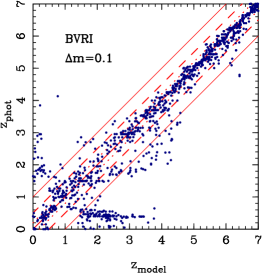
Figure 25: Same as in Fig. 25 using $BVRI$ broad-band filters. This figure is reproduced from Fig. 2 of (Bolzonella et al., 2000); dotted lines correspond to $\Delta z=0.2$, dashed lines to $\Delta z=0.5$, and thin solid lines to $\Delta z=1$, where $Deltaz=|z_{\mathrm{model}}-z_{\mathrm{phot}}|$. Conspicuous degeneracies appear along the redshift sequence.

The galaxy redshift accuracy $\sigma_{\mathrm{Res.}}\sim 0.01-0.05$ (for median $S/N\geq 10$) obtained here with the PCA should not be attributed to the PCA technique itself, but to the dense sampling of the SEDs by the LZT medium-band filters (note that $\sigma_{\mathrm{Res.}}\sim 1/R$ with the LZT filter resolution $R\simeq 40$, see Fig. 1). We illustrate this point by using another method to measure the redshifts of “LZT-observed” galaxies. We use the published code HYPERZ (Bolzonella et al., 2000) for measuring “photometric redshifts” by standard $\chi^{2}$ fits to a spectral library. The model catalog of SEDs was kindly provided by R. Pelló and is described in Bolzonella et al. (2000): it contains the SEDs with a $S/N=10$ of 1000 galaxies generated using version GISSEL98 of the GISSEL spectral library (Bruzual and Charlot, 1993; see Sect. 2.3.2). This sample was then “observed” through the LZT filters. Figure 24 shows a comparison between the input redshifts $z_{\mathrm{model}}$ of the resulting catalog with their photometric estimation $z_{\mathrm{phot}}$. In the redshift range of interest for the LZT galaxies ($0\leq z\leq 1.5$), the r.m.s. dispersion in the redshifts errors $\Delta z=|z_{\mathrm{phot}}-z_{\mathrm{model}}|$ (after rejection of the few “catastrophic detections”, defined by $\Delta z\geq 1$, and occurring only at $z\leq 0.5$), is $0.036$ in the interval $0\leq z\leq 0.5$, $0.018$ in the interval $0.5\leq z\leq 1.0$, $0.033$ in the interval $1.0\leq z\leq 1.5$. Note that these dispersions are comparable with the values obtained with the PCA in the full redshift range $0\leq z\leq 1.5$ (see Table 10).

For comparison, we replicate in Fig. 25, the $BVRI$ panel of Fig. 2 from Bolzonella et al. (2000), showing the dispersion in the photometric redshifts calculated from broad-band magnitudes with an uncertainty $\Delta m=0.1$ (which approximately matches the $S/N=10$ in the LZT SEDs used in Fig. 24): in the redshift range $0\leq z\leq 1.5$, the r.m.s. uncertainty in $z_{\mathrm{phot}}$ is in the range $0.2-0.3$ (see Table 2 of Bolzonella et al., 2000), 10 times larger than with the LZT filters. The variance in the redshifts error is also calculated after rejection of the “catastrophic detections” with $\Delta z\geq 1$. These correspond to analogous degeneracies as those described here in Sect. 6.1, and mainly occur in the redshift intervals $0\leq z\leq 0.4$ et $1.5\leq z\leq 4.5$. We emphasize that the PCA-measured redshift sequence in Fig. 24 is much cleaner than that obtained with the broad-band filters in Fig. 25. As both sets of filters span the same wavelength range, this comparison provides a direct demonstration of the general advantage of using the LZT medium-band filters over the traditional use of broad-band filters, in proportion to the resolution of the filter system used, and at the expense of observing time. An intermediate approach in which a wide-band system is complemented by medium-band filters was also proposed by Budavári et al. (2001), with a moderate gain in redshift accuracy (the error is decreased by 34% for $z\leq 1.3$).

6.3 Improvements

The measurements of physical parameters using LZT SEDs might be improved by complementing the PCA with a $\chi^{2}$ technique for measuring the redshifts. Based on spectral libraries such as those used here, a $\chi^{2}$ analysis measures redshifts to $\sigma_{\mathrm{Res.}}\la 0.02$ at $z\la 1$ for $S/N=10$ (Hickson et al., 1994). It is however very sensitive to the noise in the SEDs, as it makes use of all the information carried in them. This approach also provides a way to perform the object classification (note that at redshift $z\la 0.5$, comparison of the object profiles with the point-spread-function could be used for differentiating stars from galaxies, as discussed in Sect. 4.1). One could use the $\chi^{2}$ technique to control the redshifts calculated by the 10-component PCA, and thus identify the degenerate SEDs for which better redshifts could be measured. Alternatively, one could consider a 2-step analysis in which the $\chi^{2}$ technique is first applied to the observed SEDs in order to measure their redshifts, and in a second step, the PCA is applied to the SEDs “blue-shifted” to $z=0$, with the goal to obtain a reliable spectral classification for the identified objects, and to generate “noiseless” reconstructed SEDs. An iterative process using both techniques might be required and would contribute to improving the object classification and redshift measurement.

Because observing objects at widely different redshifts results in rest-wavelength SEDs covering differing wavelength intervals. The basic PCA technique described above and requiring that objects are covered by a common wavelength interval, could not be used on the SEDs “blue-shifted” to $z=0$. One could consider performing separate PCAs on sub-samples of rest-wavelength SEDs selected by redshift interval. Studying the evolution of the galaxy populations with redshift would however require to compare the SEDs at different redshift over a common wavelength interval. A technique, recently developed by Connolly and co-workers, uses the reconstructing ability of the PCA to fill the gaps in data with varying wavelengths intervals (Connolly & Szalay, 1999). A complementary approach which creates the spectral templates from multicolor surveys (Budavári et al., 2000) could also be applied. Overall, the resulting PCA would allow both a reliable spectral classification of all objects, and reconstruction of the missing regions of the spectra under the null-evolution hypothesis (which the PCA would implicitly do). By comparison of how the different spectral types are populated at different redshifts, such a PCA would allow one to examine and quantify the redshift evolution of the galaxy population.

7 Conclusion

This paper describes an application of Principal Component Analysis (PCA) to a simulated multicolor survey using the 40 medium-band filters of the Large Zenith Telescope. For that purpose, we generate realistic mock catalogues of $\sim 3000$ stars, $\sim 30\,000$ galaxies, and $\sim 1\,000$ QSOs. For stars, we use templates from the library of Pickles (1998) and the phenomenological model of star counts of Bahcall & Soneira (1986). For galaxies, we use spectral energy distributions (SED) from GISSEL (Charlot, 1993) and PEGASE (Fioc, 1997) and a luminosity function derived from a review of the most recent $R$-band luminosity functions of the literature. We choose the CFRS-type evolution in the galaxy luminosity function, with luminosity evolution of only the late-type galaxies. For QSOs, we use an extrapolation of the composite spectrum of Francis (1991), and the luminosity function of the 2dF QSO survey.

Using the realistic mock catalogues, we perform a PCA and extract the first 10 eigencomponents. The 10-D space allows one to separate efficiently stars, galaxies, and QSOs even at low signal-to-noise ratios. 98% of stars, 100% of galaxies and 93% of QSOs are classified correctly at a median signal-to-noise ratio $S/N=6$. These values increase to 100% of stars, 100% of galaxies and 100% of QSOs at a median $S/N=10$. For SEDs with a median $S/N=6$, the 10-component PCA also provides a measurement of redshifts accurate to $\sigma_{\mathrm{Res.}}\la 0.05$ for galaxies with $z\la 0.7$, and to $\sigma_{\mathrm{Res.}}\la 0.2$ for QSOs with $z\ga 2$. At a median $S/N=20$, $\sigma_{\mathrm{Res.}}\la 0.02$ for galaxies with $z\la 1$ and for QSOs with $z\ga 2.5$ (for a given median $S/N$, a 10 to 30 times lower $S/N$ is expected at the extreme wavelengths of the bluest/reddest objects). This is not sufficient for small-scale 3-D clustering analyses, but perfectly adequate for luminosity function studies, and for measuring the evolution with redshift in the large-scale clustering using projected moments.

This paper also underlines the main weakness of the PCA. It is well-known that age, star-formation rate, redshift, and dust extinction produce degenerate SEDs at a resolution $R\simeq 40$. Although the PCA is not able to resolve some intrinsic degeneracies due to the medium-band observing technique, it efficiently reduces the noise in the SEDs at the expense of additional degeneracies. The solution to this problem may lie in the combination of a PCA with a standard $\chi^{2}$ fitting procedure. Another crucial issue in the use of the PCA for type/class/redshift measurement, is to calculate the eigenvectors from a sample in which each type of object is sufficiently well represented. The use of such a catalog, constructed from a combination of a wide variety of well calibrated observed SEDs together with precise evolutionary models, will guarantee the best results for PCA analyses. These reference samples will also allow detection of new types of object, as these will significantly deviate from the sequences of known objects.