Io Revealed in the Jovian Dust Streams

Abstract

The Jovian dust streams are high-speed bursts of submicron-sized particles traveling in the same direction from a source in the Jovian system. Since their discovery in 1992, they have been observed by three spacecraft: Ulysses, Galileo and Cassini. The source of the Jovian dust streams is dust from Io’s volcanoes. The charged and traveling dust stream particles have particular signatures in frequency space and in real space. The frequency-transformed Galileo dust stream measurements show different signatures, varying orbit-to-orbit during Galileo’s first 29 orbits around Jupiter. Time-frequency analysis demonstrates that Io is a localized source of charged dust particles. Aspects of the particles’ dynamics can be seen in the December 2000 joint Galileo-Cassini dust stream measurements. To match the travel times, the smallest dust particles could have the following range of parameters: radius: 6 nm, density: 1.35–1.75 g/cm³, sulfur charging conditions, which produce dust stream speeds: 220$\backslash$450 km s^-1 (Galileo$\backslash$Cassini) and charge potentials: 5.5$\backslash$6.3 V (Galileo$\backslash$Cassini).

1 Overview

The Jovian dust streams are high-speed collimated streams of submicron-sized particles traveling in the same direction from a source in the Jovian system. They were discovered in March 1992 by the cosmic dust detector instrument onboard the Ulysses spacecraft, when the spacecraft was just past its closest approach to Jupiter. Observations of the Jovian dust stream phenomena continued in the next nine years. A second spacecraft, Galileo, now in orbit around Jupiter, is equipped with an identical dust detector instrument to Ulysses’ dust instrument. Before and since the Galileo spacecraft’s arrival in the Jupiter system in December 1995, investigators recorded more dust stream observations. In July and August 2000, a third spacecraft with a dust detector (combined with a chemical analyzer), Cassini, traveling on its way to Saturn, recorded more high-speed streams of submicron-sized particles from the Jovian system. The many years-long successful Jovian dust streams observations reached a pinnacle on December 30, 2000, when both the Cassini and Galileo dust detectors accomplished a coordinated set of measurements of the Jovian dust streams inside and outside of Jupiter’s magnetosphere.

Indirect methods applied by previous researchers have pointed to Io being the simplest explanation for the question of the origin of the Jovian dust streams. We first show by direct methods that Io is the source of the Jovian dust streams. To address the issue of identifying Io directly in the Galileo dust detector data, we apply time-frequency analysis, in particular, Fourier methods, to the Galileo dust data. Additional frequency signatures, such as amplitude modulation, also emerge from the time-frequency analysis.

The second part of this paper focuses on the dust streams dynamics. Here, we apply a detailed Jovian particles and fields model to simulate a dust stream particle’s trajectory as the particle moves from Io’s orbit through Jupiter’s magnetosphere and beyond. Through the model, we show one possible set of parameters that match the travel times seen in the December 30, 2000 Galileo-Cassini joint dust stream measurements.

2 Io’s Frequency Fingerprint

In order to find Io’s frequency ‘fingerprint’ in the Galileo dust detector data, we followed the following steps: 1) we transformed the Galileo dust detector data into frequency space via periodograms, 2) we noted frequency patterns such as amplitude modulations, 3) we compared the frequency-transformed Galileo data with synthetic data, and, 4) we noted spacecraft effects such as Doppler shifts.

2.1 Time-Frequency Analysis via Periodograms

The “classic” or Schuster periodogram (Bretthorst, 1988) is conventionally defined as the modulus-squared of the discrete Fourier transform. If the input time series contains a periodic feature, then the periodogram can be calculated for any frequency and it displays the presence of a sinusoid near one frequency value as a distinct peak in the spectrum. The Lomb-Scargle periodogram applied here is a slightly modified version of the classic periodogram giving a simpler statistical behavior (Scargle, 1982).

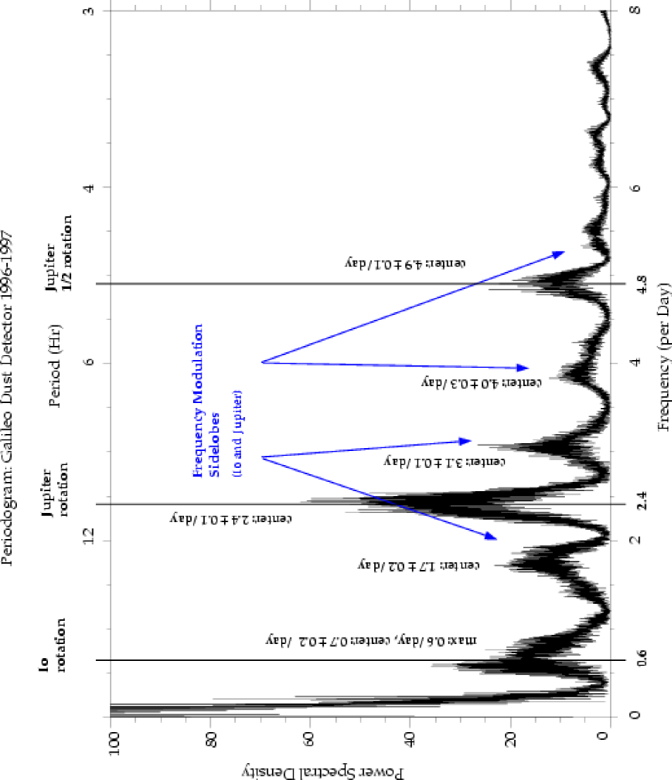
Figure 1: A Lomb-Scargle periodogram for the first two years, 1996-1997, of Galileo dust impact rate data, with the specific signatures described in the text. Io’s frequency of orbital rotation, in particular, can be seen here in frequency space, which provides our first direct evidence that Io is a source of the Jovian dust streams. A confirmation of Io’s role as a localized charged dust source arises through the modulation effects. The vertical solid lines mark Io’s orbital and Jupiter’s rotational periods, and the arrows point to Jupiter’s modulation products with Io straddling Jupiter’s frequency. The first harmonic of Jupiter’s rotation frequency is visible at ($\omega_{1}$ = 4.8 day^-1) and Jupiter’s modulation products with Io, which are straddling that first harmonic peak, can be seen, as well. The strong frequency peak near the origin at 1 over Galileo’s orbital period is due to the Galileo spacecraft orbital geometry.

Our best Galileo dust dataset for detecting Io’s frequency fingerprint emerged from the earlier Galileo orbits around Jupiter, because the spacecraft orbital geometry of the first years of the Galileo mission favored higher fluxes of dust stream particles. Therefore, by combining two years of the early data, we gained a higher signal-to-noise dataset. In Fig. 1, we show a Lomb-Scargle periodogram for the first two years, 1996-1997, of Galileo dust impact rate data. This particular periodogram is the best example from the Galileo dust detector data showing, with high confidence: Io’s frequency signature, Jupiter’s frequency signatures, and amplitude modulation effects. The periodogram shows the following frequency signatures.

Frequency Summary of Fig. 1

1. A strong peak near the origin,

2. An asymmetric peak: maximum at 0.6 day^-1, center at 0.7 $\pm$ 0.2 day^-1,

3. An asymmetric peak: center at 1.7 $\pm$ 0.2 day^-1,

4. A tall peak: center at 2.4 $\pm$ 0.1 day^-1,

5. A peak: center at 3.1 $\pm$ 0.1 day^-1,

6. Harmonics of the previous three peaks, and

7. Progressively smaller and less-defined peaks.

2.2 Amplitude Modulation in Frequency Space

Frequencies in frequency space can interact in numerous ways. We interpret the frequency peaks, seen in Fig. 1, to be the result of Io’s frequency of orbital rotation, Jupiter’s magnetic field frequency of rotation, and an interaction between these two frequencies called amplitude modulation (AM). The simplest case of AM is a sinusoid modulating the amplitude of a carrier signal, which is itself a sinusoid. Then the carrier signal is broken down in frequency space into several sinusoidal oscillations: $x\approx\sin(\omega_{0}t)+\sin(\omega_{0}t)\sin(\Omega t)$, which can be converted to sums of frequencies using a trigonometric identity for sine products. The result is a signature in frequency space that displays a carrier frequency: $\omega_{0}$ with side frequencies (“modulation products”): ($\omega_{0}+\Omega$) and ($\omega_{0}-\Omega$).

The process of amplitude modulation applies to Io’s orbital and Jupiter’s rotational frequencies in the following way. Jupiter’s rotation period is 9.8 hours corresponding to a frequency of 2.4 rotations per day. Io’s orbital period (and rotation period) is 1.8 days, corresponding to a frequency of 0.6 rotations per day. If the dust originates from Io, and the dust flux is modulated by Jupiter, then the spectrum in frequency space would appear like the spectrum in Fig. 1, where the modulation products (sidelobes) at Jupiter’s frequency at full and half-rotations are due to Jupiter’s frequency modulating Io’s frequency of orbital rotation. The frequency difference between Jupiter’s rotational frequency and each of the sidelobes is the same frequency as Io’s frequency of orbital rotation. In addition, if one or both of the original signals have broad spectra, then the spectrum of the modulation products will be broadened to the same extent (since the modulation process is linear). Therefore, the spread of Io’s peak is repeated in the same way for the sidelobes of Jupiter’s frequency peaks (full and half-rotation).

Modulation products appeared in about 20% of the first 29 frequency-transformed Galileo orbits. Galileo’s orbit E4 was the first orbit for which a hint of the amplitude modulation appeared, then in orbit G8, the signature was unmistakable. Other Galileo spacecraft orbits for which one can clearly see the modulation products are: C10, E18, and G29. Periodograms of each of the individual orbits can be seen in Graps (2001).

2.3 Synthesizing the Frequency-transformed Dust Stream Data

The main physical processes behind the frequency-transformed data can become clearer when one synthesizes data and compares the synthesized data to the real data. We have synthesized a spectrum, using typical periods from Galileo’s dust impact rate data, a Jupiter rotation and half rotation period, and an Io orbital rotational period, which show in the real data. We added some Gaussian-distributed noise, and after transforming the synthesized data into frequency space with an FFT, frequency peaks appear with their modulation products, which are in the same locations as those in the 1996-1997 Galileo dust detector periodogram. Figures of the synthesized time series and frequency-transformed data can be seen in Fig. 2.

2.4 Spacecraft Effects in Frequency Space

Several Galileo spacecraft orbital characteristics can be identified in the frequency-transformed data. The first effect is at the origin. For each orbit, the dust instrument receives more dust impacts while in the inner Jovian system than while in the outer Jovian system, which in frequency space, results in a peak at the origin. The second spacecraft effect is a Doppler effect between Galileo and Io, as the “observer” and the “source.” In frequency space, the result is that both the Io and the Jupiter peaks can be smeared by Doppler shifts. The Io frequency peak Doppler shift is to shorter periods. This asymmetry appears in the modulation products, as well. A table of the Doppler shift trends can be seen in Graps (2001).

2.5 August-September 2000 Dust Storm

In August and September 2000, both Cassini (travelling by at $\sim$1 A.U. from Jupiter), and Galileo (in an orbit carried to $\sim$250 R_J from Jupiter, where R_J=7.134 10⁹ cm is the equatorial radius of Jupiter) detected increases in the rate of dust impacts, which were approximately 100 times their nominal impact rates. In the frequency-transformed data from both spacecraft, Io’s frequency signature swamped all other frequency signatures in the Galileo data, which was noteworthy, because both spacecraft were located far from Jupiter, outside of Jupiter’s magnetosphere. Galileo detected the ‘dust storm’ earlier during the perijove portion of its G28 orbit, during Days $\sim$218–240. After Day 240, Galileo’s impact rate decreased, however, Cassini observed high impact rates particularly on $\sim$Day 251 and $\sim$Day 266. (See the periodogram of the dust impact rate in Fig. 3). Cassini’s dust detector’s observational geometry is very different from Galileo’s, however, by accident, Cassini captured the dust storm approximately 1-2 weeks after Galileo detected the dust storm.

2.6 Conclusions of Io’s Frequency Fingerprint

Frequency analysis via Fourier techniques of the Galileo dust data provides our first direct evidence of an Io dust source. The presence of Io’s rotation frequency argues that Io is a localized source of charged dust particles because charged dust from diffuse sources would couple to Jupiter’s magnetic field and appear in frequency space with Jupiter’s rotation frequency and its harmonics. A confirmation of Io’s role as a localized charged dust source arises through the modulation effects.

The Galileo dust detector periodogram data shows variabilities, orbit-to-orbit, even for some orbits which share similar orbital geometry. This orbit-to-orbit variability is a clue that, either the intervening medium or Io itself, i.e. its volcanoes, is a source of the variability.

3 Jovian Dust Stream Dynamics

To describe the dynamics of the dust streams, we apply a detailed Jovian particles and fields model to simulate a dust stream particle’s trajectory as the particle moves from Io’s orbit through Jupiter’s magnetosphere and beyond. For the model, one needs to assume approximations for the following: 1) Jupiter’s magnetic field, 2) Jupiter’s plasma, 3) dust particle density, 4) dust particle optical property, 5) charging processes, and 6) forces.

3.1 Jovian Dust Stream Model Details

We approximate Jupiter’s magnetic field by implementing Connerney’s $O_{4}$ or $O_{6}$ model (Connerney, 1981, 1993), which is a quadrupole expansion of the planet’s internal field. Additionally, we hinge Connerney’s current sheet described in Connerney et al. (1981), to approximate Jupiter’s magnetodisk. Connerney’s sheet implementation considers the magnetodisk as a perturbation to Jupiter’s internal field.

Jupiter’s plasma is approximated using a plasma model which is a fit to the Voyager 1 and 2 cold plasma measurements, described in Bagenal (1989). We assumed a constant mixing ratio of 50% between single ionized oxygen and sulfur ions.

For the dust particle density, we use density values 1.35–2.0 g/cm³. The dust particle’s optical properties are manifested via $Q_{pr}$, which affects the particle’s dynamics through the radiation pressure force. For this work, a $Q_{pr}$ value for the dust particle is calculated based on the particle’s size, and following the curve in Burns et al.’s classic paper: Burns et al. (1979).

The charge of the dust particles is approximated by summing over the currents: photoelectron emission, ion and electron collection, and secondary electron emission. The charge of the particle, which varies in time, is integrated simultaneously with the particle’s acceleration. Here, we model the acceleration by considering the following forces: Jupiter’s gravitational force, the light pressure force, the Lorentz force, and the solar gravitational force (Horányi et al., 1997). We have neglected the neutral gas and plasma (Coulomb) drag forces on the dust particle because the time-scales used in these runs are short (hours to a day), compared to the time-scales over which those forces have an effect.

More details of the Jovian dust stream model can be found in M. Horányi’s papers, such as Horányi et al. (1997), and in Graps (2001).

3.2 Dynamics Results

A window of particle sizes exists for which dust particles can escape from traveling in Keplerian orbits in Jupiter’s magnetosphere. For small dust particles, their motion is as plasma ions and electrons, which gyrate about Jupiter’s magnetic field lines. For large dust particles, their motion is governed by gravity. From Io’s orbital location, the window of dust particle sizes for escaping particles is approximately radius 5 nm to 35 nm. This particle size is strongly dependent on the charging assumptions, especially the secondary electron emission material assumption. In our numerical experiments thus far, we found that smaller dust particles can be ejected when the impacting ion or electron energy is lower than the energy of other impacting ions or electrons in the secondary electron emission process. For example, a particle with sulfur properties can be ejected from Io’s location with a minimum size 4 nm, versus a particle with silicate material properties, which can be ejected from Io’s location with a minimum size 6 nm.

As the dust stream particle moves through the Jovian magnetosphere, equilibrium potential is rarely reached. Therefore, as the particle moves outward, it continues to collect charges, which further accelerate the particle. We now think that the Jovian dust stream particles move faster (at least 400 km/sec) than previously assumed in the earlier work presented by Zook et al. (1996), which suggested dust speeds, at least 200 km/sec.

3.3 Joint Measurements: December 2000 from Galileo & Cassini

On December 30, 2000, the Cassini spacecraft closely flew by Jupiter, providing a simultaneous two-spacecraft measurement (Cassini-Galileo) of particles from one collimated stream from the Jovian dust streams. Particles in a stream were detected by Galileo, as the spacecraft was orbiting inside of the Jovian magnetosphere close to Ganymede (8–12 Jovian radii), and then particles in the stream traveled to Cassini, as Cassini flew by Jupiter at approximately 140 Jovian radii. Figure 4 shows the dust impact rate data for the dual dust stream measurements, the gold line denotes the Galileo rates and the green line indicates the Cassini rates. We assumed that the same dust stream at each spacecraft began where the black horizontal line marks the midpoint of the peak rise in impact rate. The travel time between the two black-marked peaks is approximately 7 hours. One goal of the dynamical modeling was to match this travel time. From preliminary modeling, Fig. 5 shows the result of one possible trajectory of a Jovian dust streams particle released near Io’s orbit. Here, the smallest dust particles could have the following range of parameters: size: 6 nanometers, density: 1.35–1.75 g/cm³, initial charge potential: 1–4 V, secondary electron emission yield: 3.0, dependent on a maximum electron energy 300 eV, and a photoelectron emission yield: 0.1–1.0, which produce dust particle speeds: 220$\backslash$450 km s^-1 (Galileo$\backslash$Cassini) and charge potentials: 5.5$\backslash$6.3 V (Galileo$\backslash$Cassini). Smaller and larger particles than 6 nanometers result in the wrong direction towards Cassini, and with travel times that are either too fast or too slow.

4 Synopsis

Our work from frequency analysis shows Io as the dominant source of the Jovian dust streams. The variability seen in the frequency analysis shows that we might be able to use dust stream measurements to monitor Io’s volcanoes’ plume activity.

Our charging and dynamics modeling, (more details in Graps (2001)), shows that the dust streams’ equilibrium potential is rarely reached in the Jovian magnetosphere, and that the Jovian dust stream particles travel faster than found previously in Zook et al. (1996). In our preliminary analysis and modeling of the Galileo-Cassini dust stream measurements, we show that one set of conditions, which can match the travel times, gives a dust streams speed at Galileo of 220 km s^-1, with a charge potential: 5.5 V, and a dust streams speed at Cassini of 450 km s^-1, with a charge potential: 6.3 V.

Figure 2: Top: A synthetic impact rate dataset, with added Gaussian noise, which includes the following periods: 48 days for Galileo’s orbit, 9 and 17 days for smaller data blocks, a Jupiter rotation and half rotation period, and an Io rotation period. Bottom: An FFT of the synthetic rate dataset. Galileo’s motion (at the origin), Io’s frequency of orbital rotation (0.6 d^-1), Jupiter’s full frequency (2.4 d^-1) and half-frequency (4.8 d^-1) of rotation can be seen, as well as the Io-Jupiter amplitude modulation products (sidelobes around Jupiter’s frequencies).

Figure 3: A Lomb-Scargle periodogram of dust impact rate data from Galileo (top) and Cassini (bottom) during selected days in July and August 2000. The Galileo data occurred during Galileo’s G28 orbit, when the spacecraft was located outside of Jupiter’s magnetosphere at $\sim$250 R_J(where R_J=7.134 10⁹ cm is the equatorial radius of Jupiter). This Io dust streams storm detected in interplanetary space was stronger in the earlier portion of this orbit close to perijove on Days 218–240 than in the later days, when Cassini detected the storm. Cassini observed high impact rates particularly on $\sim$Day 251 and $\sim$Day 266, when the spacecraft was traveling far outside of Jupiter’s magnetosphere at $\sim$1 A.U.

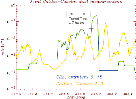
Figure 4: Dust impact rates from the Cassini-Galileo dual dust stream measurements performed on December 30, 2000. The marked travel time, 7 hours, is the time for a dust particle in a collimated dust stream to travel from Galileo to Cassini.

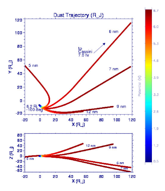
Figure 5: Dust particle trajectories in x-y (top) and x-z (bottom) Jupiter-centered coordinates for different sized particles released from a near-Io Keplerian orbit at 6.2 Jovian radii. The colors indicate the values of the particle’s charge potentials. The trajectory with the arrow indicates a reasonable trajectory which would bring the particle near to the Cassini spacecraft.

References

- Bagenal (1989) Bagenal F., 1989, In: Belton M., West R.A., Rahe J. (eds.) Time-Variable phenomena in the Jovian system, SP-494, 1–403
- Bretthorst (1988) Bretthorst G., 1988, Bayesian Spectrum Analysis and Parameter Estimation, Springer-Verlag
- Burns et al. (1979) Burns J.A., Lamy P.L., Soter S., 1979, Icarus, 40, 1
- Connerney (1981) Connerney J.E.P., Sep. 1981, J. Geophys. Res., 86, 7679
- Connerney (1993) Connerney J.E.P., Oct. 1993, J. Geophys. Res., 98, 18,659
- Connerney et al. (1981) Connerney J.E.P., Acuna M.H., Ness N.F., 1981, J. Geophys. Res., 86, 8360
- Graps (2001) Graps A.L., Jul. 2001, Io Revealed in the Jovian Dust Streams, Ph.D. thesis, Ruprecht-Karls-Universität Heidelberg
- Horányi et al. (1997) Horányi M., Grün E., Heck A., 1997, Geophys. Res. Letters, 24, 2175
- Scargle (1982) Scargle J.D., 1982, Ap. J., 263, 835
- Zook et al. (1996) Zook H.A.., Grün E., Hamilton D.P., et al., 1996, Science, 274, 1501