The Sunyaev-Zeldovich Effect in CMB-calibrated theories applied to the Cosmic Background Imager anisotropy power at $\ell>2000$

Abstract

We discuss the nature of the possible high-$\ell$ excess in the Cosmic Microwave Background (CMB) anisotropy power spectrum observed by the Cosmic Background Imager (CBI). We probe the angular structure of the excess in the CBI deep fields and investigate whether it could be due to the scattering of CMB photons by hot electrons within clusters, the Sunyaev-Zeldovich (SZ) effect. We estimate the density fluctuation parameters for amplitude, $\sigma_{8}$, and shape, $\Gamma$, from CMB primary anisotropy data and other cosmological data. We use the results of two separate hydrodynamical codes for $\Lambda$CDM cosmologies, consistent with the allowed $\sigma_{8}$ and $\Gamma$ values, to quantify the expected contribution from the SZ effect to the bandpowers of the CBI experiment and pass simulated SZ effect maps through our CBI analysis pipeline. The result is very sensitive to the value of $\sigma_{8}$, and is roughly consistent with the observed power if $\sigma_{8}\approx 1$. We conclude that the CBI anomaly could be a result of the SZ effect for the class of $\Lambda$CDM concordance models if $\sigma_{8}$ is in the upper range of values allowed by current CMB and Large Scale Structure (LSS) data.

1. Introduction

The Cosmic Background Imager (CBI) provides some of the highest resolution observations of the cosmic microwave background that have been made thus far. The observations cover the multipole range $400<\ell<4000$ which corresponds to collapsed masses ranging from a factor ten larger than the local group to the largest superclusters. These observations show, for the first time, the fluctuations on scales which gave rise to galaxy clusters and the damping of the power on small scales (Silk, 1968; Peebles & Yu, 1970; Bond & Efstathiou, 1987). Together with the results of other recent, high precision, CMB experiments (Miller et al., 1999; Netterfield et al., 2002; Lee et al., 2001; Halverson et al., 2001) the observations fit the scenario of adiabatic fluctuations generated by a period of inflationary expansion. The CBI observations also provide a unique insight into angular scales where secondary anisotropy effects are thought to become an important contribution to the power spectrum.

In a series of papers we have presented the results from the first year of CMB observations carried out by the CBI between January and December 2000. A preliminary analysis of the data was presented in Padin et al. (2001, hereafter Paper I). In Mason et al. (2003, hereafter Paper II) the observations of three differenced $45^{\prime}$ (FWHM) deep fields were used to measure the power spectrum to multipoles $\ell\lesssim 3500$ in wide bands $\Delta\ell\sim 600$. Pearson et al. (2003, hereafter Paper III) discussed the analysis of three sets of differenced $145^{\prime}\times 165^{\prime}$ mosaiced fields. Mosaicing gives a telescope a larger effective primary beam than that defined by the dish radii. This increases the resolution in the $uv$–plane due to the smaller width of the convolving function. It also reduces the effect of cosmic variance on the errors by increasing the sampled area. The mosaic fields provide high signal–to–noise ratio measurements of the power spectrum up to multipoles $\ell\sim 1700$ with a resolution $\Delta\ell=200$. Myers et al. (2003, hereafter Paper IV) give a detailed description of our correlation analysis and bandpower estimation methods. These have enabled us to analyze efficiently the large data sets involved in the CBI measurements. The implications of the results on cosmological parameters are described in Sievers et al. (2003, hereafter Paper V).

Results from the deep field observations show a fall in the power spectrum up to $\ell\sim 2000$ which is consistent with the damping tail due to the finite width of the last scattering surface. Beyond $\ell\sim 2000$ the power observed is higher than that expected from standard models of damped adiabatic perturbations which provide excellent fits to the data at larger scales. An extensive set of tests have been carried out to rule out possible systematic sources of the measured excess (Paper II). Paper III also reports results in this $\ell$-range which are consistent with those of Paper II. Since the thermal noise levels in the CBI mosaic are substantially higher in this regime than in the deep field observations, the current discussion will focus on the deep field results.

The deep field spectrum shows the power dropping to $\ell\sim 2000$, beyond which power levels are significantly higher than what is expected based on standard models for intrinsic CMB anisotropy. Assuming a single bin in flat bandpower above $\ell=2010$ the observed signal is inconsistent with zero and best–fit models at the $3.5\sigma$ and $3.1\sigma$ levels respectively. The one and two sigma confidence intervals for this bandpower are $359$–$624\,{\rm\mu K^{2}}$ and $199$–$946\,{\rm\mu K^{2}}$, respectively, with a best-fit power level of $508\,{\rm\mu K^{2}}$. The confidence limits were obtained by explicitly calculating the asymmetric, non-Gaussian likelihood of the high-$\ell$ bandpower.

A key consideration in obtaining these results is the treatment of the discrete radio source foreground. Sources with positions known from low-frequency radio surveys were projected out of the data; the brightest sources were also measured at 31 GHz with the OVRO 40-m telescope and subtracted directly from the data. The OVRO data allowed a complementary treatment of this potentially limiting population, giving us great confidence in our bright source treatment. We estimated the power level due to sources too faint to appear in the low frequency radio source catalogs from 30 GHz number counts determined from CBI and OVRO data. The contribution of these residual sources is $114\,\mu{\rm K}^{2}$— a factor of 4.5 below the observed excess— and we estimated an uncertainty of $\sim 57\,\mu{\rm K}^{2}$ in this contribution. The reader will find further discussion of both the CBI deep field spectrum and the treatment of the radio source foreground in Paper II.

Although the significance of the excess power is not conclusive it provides tantalizing evidence for the presence of secondary contributions to the microwave background anisotropies. One of the strongest expected secondary signals is the signature of the scattering of CMB photons by hot electrons in clusters known as the Sunyaev-Zeldovich (SZ) effect (Sunyaev & Zeldovich, 1970). The scattering leads to spectral distortions and anisotropies in the CMB. At the CBI observing frequencies the net effect is a decrement in the temperature along the line of sight. (However, as described in § 4, the lead-trail differencing used in the CBI observations results in positive and negative SZ signals in equal measure, so this cannot be used as a discriminating signature in our data.) The SZ effect is expected to dominate over the primary anisotropies at scales of a few arcminutes.

In this Paper we explore the possibility that the excess observed in the CBI deep fields may be a signature of the SZ effect. In § 2 we describe constraints on the normalization of the mass fluctuations $\sigma_{8}$ and shape parameter $\Gamma$ from CMB experiments and a number of independent surveys. These parameters are critical in determining the amplitude of the SZ effect over the scales of interest to the CBI results. In § 3 we show the predicted power spectra for the SZ effect for various cosmological models. We use numerical methods to estimate the contribution from the SZ effect to the CMB power spectrum. In § 4 we use simulated CBI observations of SZ ‘contaminated’ CMB realizations to investigate the effect of a SZ foreground on our bandpower estimation methods. In § 5 we extend an image filtering technique introduced in Paper IV to include specific template filters for the SZ effect. Our results and conclusions are discussed in § 6.

2. Amplitude and Shape Parameters for LSS from CMB Data

The SZ power spectrum has a strong dependence on the amplitude of the density fluctuations. The amplitude is usually parameterized by the rms of the (linear) mass fluctuations inside 8$h^{-1}$ Mpc spheres, $\sigma_{8}$. We now summarize the constraints we can obtain on the amplitude and shape of the matter power spectrum from CMB data and compare them to results from weak lensing surveys and cluster abundance data. Our parameter estimation pipeline also includes LSS priors which are designed to encompass the range in estimations from such experiments, as described below.

We use the parameter $\Gamma$ to define the shape, following Bardeen, Bond, Kaiser, & Szalay (1986, hereafter BBKS) and Efstathiou et al. (1992, hereafter EBW). A byproduct of linear perturbation calculations used to compute ${\cal C}_{\ell}$ in our database is transfer functions for density fluctuations, which can be related to LSS observables. Various (comoving) wavenumber scales determined by the transport of the many species of particles present in the universe characterize these spectra. The most important scale for dark matter dominated universes is $k^{-1}_{\rm Heq}$, that of the horizon at redshift $\Omega_{m}/\Omega_{er}$ when the density in nonrelativistic matter, $\Omega_{m}\bar{a}^{-3}$, equals that in relativistic matter, $\Omega_{er}\bar{a}^{-4}$. This defines $\Gamma_{eq}$: $k_{\rm Heq}^{-1}=5\,\Gamma_{eq}^{-1}\,h^{-1}\,{\rm Mpc}$, where $\Gamma_{eq}=\Omega_{m}\,{h}\,[\Omega_{er}/(1.68\Omega_{\gamma})]^{-1/2}$. For the cases we consider here we simply have fixed the relativistic density to correspond to the photons and three species of very light neutrinos, so $\Gamma_{eq}=\Omega_{m}\,h$.

Certain functional forms for the transfer functions are popular: In EBW a form was adopted which fit a specific $\Omega_{b}=0.03$ CDM model, but it is more general to adopt a fit to the $\Omega_{b}\rightarrow 0$ form given in BBKS appropriately corrected for the difference between the temperature of the CMB estimated then and known so well now (Bond, 1996). Although the coefficients of fits to detailed models vary with $\omega_{b},h,\omega_{m}$, which in particular result in oscillations in the transfer function for large $\omega_{b}/\omega_{m}$, it turns out that replacing $\Gamma_{eq}$ by $\Gamma$ = $\Gamma_{eq}\exp[-(\Omega_{b}(1+\Omega_{m}^{-1}(2{h})^{1/2})-0.06)]$ works reasonably well, to about 3% over the region most relevant to LSS (Sugiyama, 1995; Bond, 1996). Further, as shown in Bond (1994), replacing $\Gamma$ by $\Gamma_{\rm eff}=\Gamma+(n_{s}-1)/2$ takes into account the main effect of spectral tilt over this LSS wavenumber band. It has also been shown that the $\Gamma$-models do fit the APM and 2dFRS data reasonably well at this stage. Particularly exciting is the prospect that the baryonic oscillations may be seen, but this is not required by the data yet. The approximate codification of a vast array of models in a single $\Gamma_{\rm eff}$ variable simplifies the treatment of LSS in the CMB data enormously.

The other variable we use to construct the LSS prior is the combination $\sigma_{8}\Omega_{m}^{0.56}$. Although various fits to cluster abundances give slightly different exponents than the 0.56, the factor is consistent with a number of other measures and we adopt this form as a representative value. These invariably involve the biasing factor $b_{g}$ for the galaxies involved. For example, relating the galaxy flow field to the galaxy density field inferred from redshift surveys takes the form $[b_{g}\sigma_{8}]\,\beta_{g}$, where $\beta_{g}=\Omega_{m}^{0.56}/b_{g}$ is a numerical factor whose value depends upon data set and analysis procedure. A combination such as this also enters into redshift space distortions. A great advantage of the weak lensing and cluster abundance results shown in the figures is that they are independent of galaxy bias. However, for the cluster case, assumptions are needed which, as the spread in estimates indicates, lead to uncertainties.

Figure 1.— One-dimensional projected likelihood functions of $\sigma_{8}$ calculated for the CMB data with three prior probability restrictions on the cosmological parameters are contrasted with estimates from other datasets. The curves shown used ‘all-data’ for the CMB available for Paper V, namely DMR, DASI (Halverson et al., 2001), BOOMERANG (for the Ruhl et al. (2003) cut), MAXIMA (Lee et al., 2001), VSA (Scott et al., 2002) and the CBI mosaic data for the odd $\Delta L$=140 binning. The marginalization has been performed over seven cosmological variables and all of the relevant calibration and beam uncertainty variables associated with the experiments, seven in this case. Application of the weak-h prior is long-dashed blue, of the flat weak-h prior is solid black and of the LSS flat weak-h prior is dotted black. Adding TOCO (Miller et al., 1999), the Boomerang test flight and 17 other experiments predating April 1999 (hereafter ‘April 99’) as well gives very similar results. The Bayesian 50% and associated 16% and 84% error bars are shown as data points in blue for these and other priors, in particular those with the stronger HST measurement of $h$ included and with SN data included. The magenta data points with smaller errors are those determined with ‘all-data’ to March 2003, including WMAP, as described in Bond et al. (2003). The original LSS prior was constructed based on the cluster abundance data (Bond, 1996; Bond & Jaffe, 1999; Lange et al., 2001). An SZ estimate of $\sigma_{8}$ from Goldstein et al. (2003) that simultaneously determines amplitudes for a best-fit primordial spectrum and an SZ spectrum for our CBI deep field data in conjunction with ACBAR (Kuo et al., 2004) and BIMA (Dawson et al., 2002) data is shown at the top. Estimates of $\sigma_{8}$ from cluster abundance data and from weak lensing data are also shown. These results have invariably had more restrictive priors imposed than those for the CMB, and so are not always applicable, but the overall level of agreement in the various approaches is encouraging. From top to bottom, the sample cluster values are from Eke et al. (1996); Carlberg et al. (1997); Fan & Bahcall (1998); Pen (1998c); Pierpaoli, Scott & White (2001); Reiprich & Böhringer (2002); Seljak (2002); Viana, Nichol & Liddle (2001); Borgani et al. (2001), then two estimates from Pierpaoli et al. (2003), then from Schuecker et al. (2003); Allen et al. (2003); Voevodkin & Vikhlinin (2004). From top to bottom, the weak lensing estimates are from Hoekstra et al. (2002); van Waerbeke et al. (2002); Refregier et al. (2002); Bacon et al. (2002); Jarvis et al. (2003); Hamana et al. (2003); Brown et al. (2003); Heymans et al. (2004).

Figure 2.— The weak prior we use for LSS in $\sigma_{8}\Omega_{m}^{0.56}$ is compared with estimates from SZ, cluster abundances, weak lensing and from the CMB data shown in Fig. 1, appropriately scaled. The blue error bars are for ‘all-data’ to June 2002, and the magenta are for ‘all-data’ to March 2003. The prior used in past work was shifted up in central value from 0.47 to 0.55, but was otherwise the same. We have also considered the LSS(low-$\sigma_{8}$) case (dashed green), with the prior shifted downward to be centered on 0.40 to accommodate better the low cluster abundance estimates, with results shown in Tables 2, 3.

In Figures 1 and 2 we show the effect of the different priors on the distributions of $\sigma_{8}$ and $\sigma_{8}\Omega_{m}^{0.56}$, respectively. We also compare these to the weak lensing results shown in the figures. The “Red Cluster Survey” results of Hoekstra et al. (2002) and the “Virmos-Descart Survey” results of van Waerbeke et al. (2002) correspond to a version of a weak prior: they marginalize over $\Gamma_{\rm eff}$ in the range 0.1 to 0.4, which is largely equivalent for this application to marginalization over $\omega_{b}$, $n_{s}$ and $\omega_{m}$. They also marginalize over the uncertainty in the mean redshift of the lensed galaxies $z_{s}$ from 0.27 to 0.34 in the former case, and 0.78 to 1.08 in the latter case. On the other hand, the cosmology was kept fixed with $\Omega_{m}=0.3$. Refregier et al. (2002) and Bacon et al. (2002) adopt a more restrictive parameter range. If the weak marginalization scheme of Hoekstra et al. (2002) and van Waerbeke et al. (2002) were used the error bars would increase in these cases. (Recently van Waerbeke et al. (2005) have improved the Virmos-Descart Survey analysis, which lowers the van Waerbeke et al. (2002) $\sigma_{8}$ estimate by 12%.)

Figs. 1 and 2 show sample cluster abundance estimates of $\sigma_{8}$ which are discussed below.

Figure 3.— The prior probability used for the shape parameter $\Gamma_{\rm eff}$ is shown as solid green. (This is to be contrasted with the more skewed one used in Lange et al. (2001), etc., shown as light dashed-dotted green.) The $\Gamma$-prior was designed to encompass the range indicated by the APM data, vintage 1992, but estimates from the 2dFRS and SDSS shown below are quite compatible. The CMB results for $\Gamma_{\rm eff}$ are shown with various choices for priors for comparison. Solid blue is for ‘all-data’ as of June 2002, as described in Sievers et al. (2003), and magenta is for the data as of March 2003, as described in Bond et al. (2003). $\Gamma_{\rm eff}$ includes corrections for $\omega_{b}$, $h$, and the tilt. The related values of $\Omega_{m}h$ are shown at the bottom to show the effect of these corrections.

van Waerbeke et al. (2002) give a weak lensing result of $\Gamma_{\rm eff}=0.25\pm 0.13$ with marginalization over $\Omega_{m}$ from 0.1 to 0.4 and over $\sigma_{8}$. This is not explicitly shown in Fig. 3 where we plot the prior probability we adopted for $\Gamma_{\rm eff}$. The APM result is the long standing one used to construct the original prior, that $\Gamma_{\rm eff}$ in the 0.15 to 0.3 range provided a good fit to the data, e.g. EBW and Bond (1996). Recent 2dFRS (Peacock et al., 2001) and SDSS (Szalay et al., 2001) results shown give compatible results. Dodelson et al. (2001) estimate $0.14^{+0.11}_{-0.06}$, with errors at 95% confidence, for SDSS. Szalay et al. (2001) also give an estimate of $\sigma_{8}$ of $0.92\pm 0.06$, but the issue of galaxy biasing is folded into this determination. Although there are indications from the 2dF survey that biasing for the relevant galaxies is nearly unity from redshift-space distortions ($b=1.04\pm 0.11$, Verde et al. 2002), and the result is therefore compatible with the results shown, such results are not as directly applicable as those from clusters and from lensing which directly relate to matter density power spectrum amplitudes.

The LSS prior used here and in Paper V involves a combination of constraints on the amplitude parameter $\sigma_{8}\Omega_{m}^{0.56}$ and on the shape parameter $\Gamma_{\rm eff}$. It differs slightly from that used in Lange et al. (2001), Jaffe et al. (2001) and Netterfield et al. (2002). We use $\sigma_{8}\Omega_{m}^{0.56}$=$0.47^{+0.02,+0.11}_{-0.02,-0.08}$, distributed as a Gaussian (first error) smeared by a uniform (tophat) distribution (second error). We constrain the shape of the power spectrum via $\Gamma_{\rm eff}\equiv\Gamma+(n_{s}-1)/2$=$0.21^{+0.03,+0.08}_{-0.03,-0.08}$, where $\Gamma\approx\Omega_{m}\,h\,\,e^{-[\Omega_{B}(1+\Omega_{m}^{-1}(2{h})^{1/2})-0.06]}$. In earlier work a central value of $\sigma_{8}\Omega_{m}^{0.56}=0.55$ was used together with $\Gamma_{\rm eff}$ = $0.22^{+0.07,+0.08}_{-0.04,-0.07}$. The old $\Gamma$ prior is compared with the current version in Fig. 3. The change does not affect the parameter values obtained.

The original $\sigma_{8}$ prior choice was motivated by fits to the cluster temperature distribution, as was the decision to lower the central value by 15% made here. Our philosophy is to make the distribution broad enough so that reasonable uncertainties are allowed for in the prior. For example, there are many models that do not fit the shape as well as the amplitude of the cluster distribution function. Thus the best $\sigma_{8}$ for a given model depends upon the temperature range chosen for the fit, and other physics might be involved. Especially with the reduced model spaces often considered, the formal statistical errors can look spectacularly good, but systematic issues undoubtedly dominate. Curiously, with the 15% drop, it appears that the $\sigma_{8}$ prior chosen could have been designed for the (weak) weak lensing results. We test sensitivity by showing results for a ‘LSS(low-$\sigma_{8}$)’ prior which has a further drop of 15%: $\sigma_{8}\Omega_{m}^{0.56}$=$0.40^{+0.02,+0.11}_{-0.02,-0.08}$, This also accommodates some of the recent lower $\sigma_{8}$ estimates from cluster abundances, many of which use the X-ray luminosity as an indicator of mass, calibrated by observations. (We note that the re-analyzed Virmos-Descart Survey result (van Waerbeke et al., 2005) gives $\sigma_{8}\Omega_{m}^{0.56}$=$0.43\pm 0.04$, similar to the value obtained from the CMB-only data when WMAP is included.)

We will discuss the simulations in detail below, but we note here that the cases we have run simulations on have $\sigma_{8}=0.9$ and $1.0$, and $\Gamma_{\rm eff}=0.18$ and $0.21$. The detailed baryonic dependence of the transfer function was included in the $0.18$ case. The parameter choices were $\omega_{b}=0.022$ and $0.0245$, $h=0.7$, $\Omega_{m}=0.3$ and $0.37$. A best-fit model to the data for many prior choices has $\omega_{b}=0.0225,\omega_{c}=0.12,n_{s}=0.95,\tau_{C}=0.1$, and $\Omega_{\Lambda}=0.7$ and with $h=0.69,\Omega_{b}=0.047,\Omega_{\rm cdm}=0.253$ with a 13.7 Gyr age; the normalization is $\sigma_{8}=0.84$, and $\Gamma=0.17$ with $\Gamma_{\rm eff}=0.15$.

In general, CMB data provide weak constraints on the normalization of the matter fluctuations due to the added effects of the spectral tilt $n_{s}$ and the optical depth parameter $\tau_{C}$ on the overall amplitude of the CMB power spectrum. Allowing for tensor modes in the power spectrum introduces further degeneracies. As shown in Paper V, when fitting for a given parameter we adopt the conservative, and more computationally intensive, approach of marginalizing over all other variables considered.

Table 1Simulation parameters

Code	Size (Mpc)	Resolution	$\sigma_{8}$	$\Omega_{b}h^{2}$	$\Omega_{\Lambda}$	$\Omega_{m}$	$h$	$n_{s}$	$\Gamma_{\rm eff}$
SPH	$200$	$256^{3}$	$0.9$	$0.0200$	$0.70$	$0.30$	$0.70$	$1.0$	$0.18$
SPH	$200$	$256^{3}$	$1.0$	$0.0200$	$0.70$	$0.30$	$0.70$	$1.0$	$0.18$
SPH	$400$	$512^{3}$	$0.9$	$0.0220$	$0.70$	$0.30$	$0.70$	$1.0$	$0.18$
MMH	$143$	$512^{3}$	$1.0$	$0.0245$	$0.63$	$0.37$	$0.70$	$1.0$	$0.21$

Table 2Amplitude and Shape Parameters for LSS from the CMB: ‘all–data’, June 2002 Compilation

Priors	$\sigma_{8}$	$\sigma_{8}\Omega_{m}^{0.56}$	$\Gamma_{eq}$	$\Gamma$	$\Gamma_{\rm eff}$
wk-$h$	$0.88^{0.13}_{0.12}$	$0.61^{0.16}_{0.22}$	$0.28^{0.07}_{0.07}$	$0.23^{0.06}_{0.06}$	$0.21^{0.05}_{0.05}$
wk-$h$+LSS	$0.83^{0.11}_{0.10}$	$0.52^{0.06}_{0.11}$	$0.23^{0.04}_{0.04}$	$0.20^{0.04}_{0.04}$	$0.18^{0.03}_{0.03}$
wk-$h$+LSS(low-$\sigma_{8}$)	$0.81^{0.10}_{0.10}$	$0.45^{0.06}_{0.08}$	$0.21^{0.04}_{0.04}$	$0.17^{0.04}_{0.04}$	$0.17^{0.03}_{0.03}$
wk-$h$+SN	$0.85^{0.15}_{0.12}$	$0.45^{0.11}_{0.08}$	$0.21^{0.03}_{0.03}$	$0.17^{0.03}_{0.03}$	$0.17^{0.03}_{0.03}$
flat+wk-$h$	$0.89^{0.10}_{0.11}$	$0.56^{0.23}_{0.25}$	$0.26^{0.08}_{0.08}$	$0.23^{0.08}_{0.08}$	$0.20^{0.07}_{0.07}$
flat+wk-$h$+LSS	$0.87^{0.08}_{0.07}$	$0.50^{0.07}_{0.11}$	$0.23^{0.04}_{0.04}$	$0.20^{0.04}_{0.04}$	$0.17^{0.03}_{0.03}$
flat+wk-$h$+LSS(low-$\sigma_{8}$)	$0.84^{0.09}_{0.08}$	$0.43^{0.06}_{0.09}$	$0.20^{0.04}_{0.04}$	$0.17^{0.03}_{0.03}$	$0.15^{0.03}_{0.03}$
flat+wk-$h$+SN	$0.85^{0.11}_{0.09}$	$0.43^{0.10}_{0.11}$	$0.20^{0.03}_{0.03}$	$0.17^{0.03}_{0.03}$	$0.15^{0.03}_{0.03}$
flat+HST-$h$	$0.86^{0.11}_{0.11}$	$0.44^{0.13}_{0.16}$	$0.21^{0.05}_{0.05}$	$0.18^{0.05}_{0.05}$	$0.16^{0.04}_{0.04}$
flat+HST-$h$+LSS	$0.88^{0.08}_{0.08}$	$0.47^{0.08}_{0.07}$	$0.22^{0.03}_{0.03}$	$0.19^{0.03}_{0.03}$	$0.17^{0.03}_{0.03}$
flat+HST-$h$+SN	$0.84^{0.11}_{0.08}$	$0.43^{0.08}_{0.08}$	$0.20^{0.03}_{0.03}$	$0.17^{0.03}_{0.03}$	$0.15^{0.03}_{0.03}$
flat+HST-$h$+LSS+SN	$0.87^{0.09}_{0.08}$	$0.45^{0.07}_{0.05}$	$0.21^{0.02}_{0.02}$	$0.18^{0.02}_{0.02}$	$0.16^{0.03}_{0.03}$
flat+HST-$h$+LSS(low-$\sigma_{8}$)+SN	$0.85^{0.09}_{0.07}$	$0.43^{0.05}_{0.05}$	$0.20^{0.02}_{0.02}$	$0.17^{0.02}_{0.02}$	$0.15^{0.02}_{0.02}$

Note. — Amplitude and shape parameter estimates from various datasets, for various prior probability choices and using ‘all-data’ for the CMB available for Paper V, and as described there, in particular DMR+DASI+MAXIMA + BOOMERANG (Ruhl et al. 2003 cut), VSA and CBI mosaic data for the odd $\Delta\ell$=140 binning, as described in Paper III. In the first four rows, the weak prior in $h$ ($0.45<h<0.90$) is imposed (including further weak constraints on cosmological age, $t_{0}>10$ Gyr, and matter density, $\Omega_{m}>0.1$). The sequence shows what happens when priors for LSS (with $\sigma_{8}\Omega_{m}^{0.56}$ centered about 0.47), for LSS(low-$\sigma_{8}$) (with the $\sigma_{8}$ distribution shifted downward by 15%, centered about 0.40), and for SN are imposed. While the first four rows allow $\Omega_{tot}$ to be free, the next four have $\Omega_{tot}$ pegged to unity, a number strongly suggested by the CMB data. The final 4 rows show the ‘strong-$h$’ prior, a Gaussian centered on $h=0.71$ with dispersion $\pm 0.07$, obtained for the Hubble key project. The $t_{0}>10$ Gyr and $\Omega_{m}>0.1$ constraints are also imposed, but they have no impact. Central values and $1\sigma$ limits for the 7 database parameters that form our fiducial minimal-inflation model set are found from the 16%, 50% and 84% integrals of the marginalized likelihood for $\sigma_{8}$ and $\sigma_{8}\Omega_{m}^{0.56}$. For $\Gamma_{eq}\equiv\Omega_{m}h$, $\Gamma$ and $\Gamma_{\rm eff}$, the values are means and variances of the variables calculated over the full probability distribution. Shifting the center of the $\sigma_{8}\Omega_{m}^{0.56}$ prior downward by 15% to accommodate more of the low cluster results has little effect on the flat+HST-$h$+LSS+SN result.

In Table 2 we summarize the constraints on the LSS parameters from the CMB data used in Paper V and a combination of priors. The mean and quoted ($1\sigma$) errors correspond to the 50%, 16% and 84% integrals of the marginalized likelihoods respectively.

Figure 4.— One and two sigma contours of 2D projected likelihood functions show how various cosmological parameters correlate with $\sigma_{8}$. For this case, ‘all–data’ from the June 2002 compilation was used: DASI+MAXIMA+BOOMERANG+VSA plus the CBI mosaic data for the odd $\Delta L$=140 binning. The $\Omega_{k}-\sigma_{8}$ panel shows the weak-$h$ prior (magenta) and LSS+weak-$h$ prior (solid black). For the other 3 panels the flat constraint was added to these two priors as well. Note the positive correlation with $n_{s}$, but little correlation in the other variables.

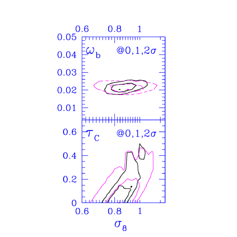
Figure 5.— One and two sigma contours of 2D projected likelihood functions for $\omega_{b}$ and $\tau_{C}$ for ‘all-data’ of Sievers et al. (2003). The flat+weak-$h$ prior (magenta) and flat+LSS+weak-$h$ prior (solid black) cases are shown. The significant $\sigma_{8}$–$\tau_{C}$ correlation is evident, which results in a higher $\sigma_{8}$ for higher $\tau_{C}$. One could impose a stronger prior than $\tau_{C}<0.7$ (as is done here) based on astrophysical arguments. This is fraught with uncertainty since it involves the first objects collapsing on small scales in the universe and their efficiency in generating stars that produce ionizing radiation. However, $\tau_{C}$ has apparently been detected by WMAP at the $0.16\pm 0.04$ level (Kogut et al., 2003), and results with a prior encompassing this detection on the March 2003 compilation of the data are given in Table 3.

In Figs. 4 and 5 we show the correlation of $\sigma_{8}$ with other parameters considered. Correlations with $\tau_{C}$ are nontrivial, and allowing the space to be open in $\tau_{C}$ does tend to give higher marginalized $\sigma_{8}$. The CMB data as of June 2002 did not give an indication of a $\tau_{C}$ detection, and we have imposed no physical prior on those results.

Table 3Amplitude and Shape Parameters for LSS from the CMB: ’all–data’, March 2003 Compilation

Priors	$\sigma_{8}$	$\sigma_{8}\Omega_{m}^{0.56}$	$\Gamma_{eq}$	$\Gamma$	$\Gamma_{\rm eff}$
wk-$h$	$0.83^{0.04}_{0.06}$	$0.45^{0.24}_{0.16}$	$0.24^{0.07}_{0.07}$	$0.20^{0.06}_{0.06}$	$0.18^{0.05}_{0.05}$
wk-$h$+LSS	$0.85^{0.04}_{0.03}$	$0.44^{0.02}_{0.02}$	$0.21^{0.02}_{0.02}$	$0.17^{0.01}_{0.01}$	$0.15^{0.02}_{0.02}$
wk-$h$+LSS(low-$\sigma_{8}$)	$0.84^{0.05}_{0.05}$	$0.43^{0.02}_{0.04}$	$0.20^{0.02}_{0.02}$	$0.17^{0.02}_{0.02}$	$0.15^{0.02}_{0.02}$
wk-$h$+SN	$0.84^{0.05}_{0.05}$	$0.43^{0.02}_{0.13}$	$0.20^{0.02}_{0.02}$	$0.17^{0.02}_{0.02}$	$0.14^{0.02}_{0.02}$
flat+wk-$h$	$0.83^{0.05}_{0.06}$	$0.43^{0.03}_{0.16}$	$0.19^{0.03}_{0.03}$	$0.16^{0.03}_{0.03}$	$0.14^{0.02}_{0.02}$
flat+wk-$h$+LSS	$0.85^{0.04}_{0.03}$	$0.44^{0.02}_{0.02}$	$0.21^{0.01}_{0.01}$	$0.17^{0.01}_{0.01}$	$0.15^{0.01}_{0.01}$
flat+wk-$h$+LSS(low-$\sigma_{8}$)	$0.84^{0.05}_{0.05}$	$0.43^{0.02}_{0.04}$	$0.20^{0.02}_{0.02}$	$0.17^{0.02}_{0.02}$	$0.15^{0.02}_{0.02}$
flat+wk-$h$+SN	$0.84^{0.05}_{0.05}$	$0.43^{0.02}_{0.13}$	$0.20^{0.02}_{0.02}$	$0.17^{0.02}_{0.02}$	$0.14^{0.02}_{0.02}$
flat+HST-$h$	$0.83^{0.05}_{0.06}$	$0.43^{0.02}_{0.16}$	$0.19^{0.03}_{0.03}$	$0.16^{0.03}_{0.03}$	$0.14^{0.02}_{0.02}$
flat+HST-$h$+LSS	$0.85^{0.04}_{0.03}$	$0.44^{0.02}_{0.02}$	$0.21^{0.01}_{0.01}$	$0.17^{0.01}_{0.01}$	$0.15^{0.01}_{0.01}$
flat+HST-$h$+SN	$0.84^{0.04}_{0.05}$	$0.43^{0.02}_{0.04}$	$0.20^{0.02}_{0.02}$	$0.17^{0.02}_{0.02}$	$0.15^{0.02}_{0.02}$
flat+HST-$h$+LSS+SN	$0.85^{0.04}_{0.03}$	$0.44^{0.02}_{0.02}$	$0.21^{0.01}_{0.01}$	$0.17^{0.01}_{0.01}$	$0.15^{0.01}_{0.01}$
flat+HST-$h$+LSS(low-$\sigma_{8}$)+SN	$0.85^{0.04}_{0.04}$	$0.44^{0.02}_{0.03}$	$0.20^{0.02}_{0.02}$	$0.17^{0.02}_{0.02}$	$0.15^{0.02}_{0.02}$

Note. — Similar to Table. 2 but for an extension of ‘all-data’ to include WMAP, ACBAR, extended VSA ((Grainge et al., 2003)) and CBI results, as well as DASI, Boomerang and Maxima, analyzed in the same way. A further (weak) prior on $\tau_{C}$ was applied to accommodate the WMAP detection from the cross-correlation of temperature and polarization, but this makes little difference to the results. For example, without this extra prior, flat+wk-$h$ shifts to $0.81^{0.05}_{0.05}$ and $0.41^{0.03}_{0.11}$. As for Table 2, the downshifted LSS prior has little effect on flat+HST-$h$+LSS+SN.

The addition of the first-year WMAP data and other data that has appeared since sharpens the determination of the parameters $\sigma_{8}$, $\sigma_{8}\Omega_{m}^{0.56}$ and $\Gamma_{\rm eff}$. This ‘March 2003’ compilation of CMB anisotropy data, described in Bond et al. (2003), is treated in the same way as the June 2002 data is in Paper V, with the same ${\cal C}_{\ell}$-database. Results are shown in Table 3 and in the reduced errors in Figs. 1, 2 and 3. For the March 2003 data, a prior was included on $\tau_{C}$ to accommodate the $\tau_{C}=0.16\pm 0.04$ detection reported by the WMAP team (Kogut et al., 2003). The form we have adopted has a top-hat spread convolved with a Gaussian distribution, as for our $\sigma_{8}\Omega_{m}^{0.56}$ and $\Gamma_{\rm eff}$ priors: $\tau_{C}=0.16^{+0.04,+0.06}_{+0.04,+0.06}$. Similar results are obtained using the Markov Chain Monte Carlo approach, which explicitly includes the $\tau_{C}$-detection using the TE data of Kogut et al. (2003).

Best-fit models may have lower $\sigma_{8}$ values than the marginalized values. Typical best–fit models for the June 2002 dataset are: ($\Omega_{\rm cdm}=0.47,\Omega_{\Lambda}=0.50,\Omega_{b}=0.079,h=0.51,n_{s}=0.90,\tau_{C}=0$ and $\sigma_{8}=0.72$) for the weak prior case and ($\Omega_{\rm cdm}=0.44,\Omega_{\Lambda}=0.50,\Omega_{b}=0.063,h=0.57,n_{s}=0.90,\tau_{C}=0$ and $\sigma_{8}=0.81$) for flat+weak and flat+weak+LSS priors. These $\sigma_{8}$ values are lower because the best–fits selected the $\tau_{C}=0$ peak in the likelihood whereas integration over the relatively broad $\tau_{C}$ likelihood allows for the inclusion of high–$\sigma_{8}$ models. If the HST-$h$ or SN prior is included along with LSS, the best-fit model is a more conventional $\Lambda$CDM one, with $\tau_{C}=0.1$: ($\Omega_{\rm cdm}=0.25,\Omega_{\Lambda}=0.70,\Omega_{b}=0.047,h=0.69,n_{s}=0.95,\tau_{C}=0.1$ and $\sigma_{8}=0.84$). For the March 2003 data with the $\tau_{C}$ prior, this $\tau_{C}=0.1$ model also provides a best-fit for the weak+flat and weak+flat+LSS cases.

Comparison of our results with independent estimates of $\sigma_{8}$ from CMB data is complicated by the different choices of parameter marginalization and by different treatments of the CMB data. Lahav et al. (2002) carried out a joint CMB–2dFRS analysis of cosmological parameters. Their result is $\sigma_{8}=0.73\pm 0.05$ after marginalizing over some variables but keeping $\tau_{C}$ fixed at 0 and $n_{s}$ fixed at unity. This value is therefore biased low with respect to non–zero $\tau_{C}$ models. They also show how letting $\tau_{C}$ vary gives higher values for $\sigma_{8}$. Melchiorri & Silk (2002) quote smaller values for $\sigma_{8}$ in their analysis, even when $\tau_{C}$ was allowed to vary.

The values we obtain for the March 2003 dataset are in good agreement with those obtained by the WMAP team (Spergel et al., 2003). However we caution that the projected distribution of $\sigma_{8}$ from the CMB depends upon the other parameters. For the seven-parameter inflation-motivated models considered here, there is a strong correlation of $\sigma_{8}$ with the Thomson scattering depth $\tau_{C}$ and the primordial spectral index $n_{s}$. If, in addition, $n_{s}$ is allowed a logarithmic correction with wavenumber, introducing another parameter highly correlated with $\sigma_{8}$, the distribution extends to higher $\sigma_{8}$ (Bond et al., 2003). Allowing for a gravity wave contribution extends the distribution to lower $\sigma_{8}$. These caveats about the effect of adding extra parameters in the CMB analysis together with the scatter in the estimates of $\sigma_{8}$ from clusters and weak lensing shown in Figs. 1 and 2 reflect the current uncertainty as to whether a low or high $\sigma_{8}$ will emerge.

3. The Angular Power Spectrum of the Sunyaev-Zeldovich Effect

The SZ effect is a signature of the scattering of CMB photons off hot electrons. The effect can be described in terms of the fractional energy gain per scatter along the line of sight. By multiplying by the number density of electrons and integrating along the line of sight we can derive the induced temperature change:

$$\frac{\Delta T_{\rm SZ}}{T_{\rm CMB}}=-2y\,\psi_{K}(x)=-2\sigma_{T}\int n_{e}\frac{k_{B}(T_{e}-T_{\rm CMB})}{m_{e}c^{2}}d\chi\,\psi_{K}(x)\,,$$ (1)

where $y$ is the Compton $y$-parameter, $\sigma_{T}$ is the Thomson cross–section, $n_{e}$ is the electron number density, $T_{e}$ is the electron temperature, $T_{\rm CMB}$ is the CMB temperature, $k_{B}$ is Boltzmann’s constant and $m_{e}c^{2}$ is the electron’s rest mass energy. Here $\psi_{K}(x),\,x\equiv h\nu/k_{B}T_{\rm CMB}$ is a frequency-dependent function which is unity at Rayleigh-Jeans wavelengths and is 0.975 at the 30 GHz frequencies probed by the CBI.

With the great increase in experimental sensitivity, measurement of the SZE in known clusters has become almost routine (see, e.g., Birkinshaw, Gull & Hardebeck 1984; Carlstrom et al. 1996; Holzapfel et al. 1997; Mason, Myers, & Readhead 2001; Udomprasert et al. 2004; Grainge et al. 2002). Coupled with X–ray observations of the cluster these measurements yield independent constraints on the value of the Hubble constant. They also provide a direct measurement of the amount of baryon mass in the cluster gas. The SZ effect is expected to contribute significantly to the CMB power spectrum at scales $\ell>2000$, with a crossover point between the primary CMB and SZ signature occuring somewhere between $\ell\sim 2000$ and $\ell\sim 3000$. Surveys observing at these scales will therefore require accurate component separation to reconstruct the primary CMB spectrum and much work has focused on this issue in recent years. Many proposed experiments will adopt multi-frequency observing strategies in order to separate the different components by their different spectral dependence. These techniques cannot be applied to the narrow frequency band of the CBI observations. However we can attempt to address the question of whether the SZ effect could provide a contribution with the required amplitude to explain the observed excess.

We use the output of two separate hydrodynamical simulation algorithms in an attempt to predict the level at which the SZ effect will contribute to the CBI deep field observations. We also relate our numerical results to analytical models of the SZ power spectrum based on the halo model.

3.1. Hydrodynamical Simulations of the Sunyaev-Zeldovich Effect

The two codes that we have employed both provide high-resolution dark matter and hydrodynamical simulations of large scale cosmic structure which we use to generate simulated wide-field SZ maps. The simulation algorithms and processing techniques were developed independently (Pen, 1998a; Bond et al., 1998, 2002; Wadsley, Stadel & Quinn, 2003) and are based on two different numerical schemes for solving the self–gravitating, hydrodynamical equations of motion. High-resolution gasdynamical simulations of large enough volumes are still beyond current technological capabilities. Following an approach taken previously by other authors (e.g., Springel, White & Hernquist, 2001), we create a pseudo-realization of the cosmic structure up to high redshifts from a single, medium-sized, high-resolution simulation by stacking randomly translated and rotated (or flipped) copies of the (evolving) periodic volume.

One set of SZ simulations was obtained using the Gasoline code, an efficient implementation of the (Lagrangian) smooth particle hydrodynamics (SPH) method (Wadsley, Stadel & Quinn, 2003). This tree$+$SPH code uses a pure tree-based gravity solver and has spatially-adaptive time stepping. It has been parallelized on many architectures (MPI in this case) and shows excellent scalability. The results presented here are based on the analysis of three high resolution $\Lambda$CDM simulations: two 200 Mpc box computations, with $256^{3}$ dark matter plus $256^{3}$ gas particles, and one 400 Mpc box computation, with $512^{3}$ dark and $512^{3}$ gas particles, a very large number for SPH simulations. The calculations were adiabatic, in the sense that only shocks could inject entropy into the medium. Despite the different sizes, all three simulations were therefore run with the same mass resolution. All simulations were run with a gravitational softening of 50 kpc (physical). The scale probed by the SPH smoothing kernel was not allowed to become smaller than the gravitational softening in the 200 Mpc runs, but it was not limited in the 400 Mpc run, which attained gas resolution scales as low as 5 kpc in the highest density environments, though increasing considerably at lower density. (64 neighbors were required to be within the smoothing kernel in the 400 Mpc run.) The $512^{3}$ simulation was performed on a large-memory, 114 (667 MHz) processor SHARCNET COMPAQ SC cluster at McMaster University. It required about 80 GB of memory and took $\sim 40$ days of wall time to run.

Another set of SZ maps was obtained using a $512^{3}$ run of the Moving Mesh Hydrodynamics (MMH) code of Pen (1998a). This code features a full curvilinear Total-Variation-Diminishing (TVD) hydro code with a curvilinear particle mesh (PM) N-body code on a moving coordinate system. We follow the mass field such that the mass per unit grid cell remains approximately constant. This gives all the dynamic range advantages of SPH simulations combined with the speed and high resolution of grid algorithms. The box size was $143$ Mpc and the smallest grid spacing was $57$ kpc (comoving). This $512^{3}$ simulation used $30$ GB memory and took about three weeks ($\sim 1500$ steps) on a 32 processor shared memory Alpha GS320 using Open MP parallelization directives. The calculations were adiabatic as well.

The simulation boxes yield a number of projections of the gas distributions in random orientations and directions. The projections are then stacked to create a redshift range appropriate for the SZ simulation. In the case of the MMH simulation the angular size of the simulated box above a redshift of $z=1.6$ is smaller than $2$ degrees, the required angular size of the SZ simulations. To include the contributions from higher redshifts we tiled two copies of the periodic box to cover the increased angles. This only affects the smallest scales. All the maps were obtained with a low redshift cutoff at $z=0.2$ to minimize the contribution from the closest clusters in the projections. The computational costs of running such large hydrodynamical simulations prevented us from obtaining targeted simulations with identical cosmological parameters from both algorithms. Below we account for the parameter variations in the models run when comparing the two simulations and we see a remarkable consistency between the results. The parameter variations are, in fact, an advantage for us since they provide us with a sampling of the SZE amplitude for processing through the CBI pipeline. We summarize the parameters used in the simulations in Table 1.

The two 200 Mpc SPH simulations were used to generate 20 2$\times$2 degree maps each while the MMH simulation yielded 40 separate maps. A detailed analysis of the MMH maps including SZ statistics and non-Gaussianity is given by Zhang, Pen & Wang (2002). A preliminary analysis of simulated SZ maps based on one of the $256^{3}$ SPH simulations was presented by Bond et al. (2002), and a more detailed analysis of the $512^{3}$ results will be presented elsewhere.

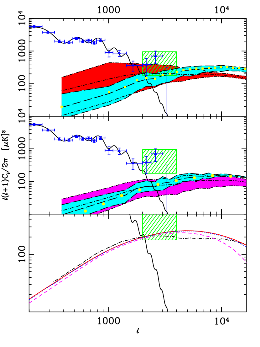
Figure 6.— SZ power spectra for various simulations. All SZ spectra have been scaled to a common $\Omega_{b}h=0.0314$, the best–fit to the CMB data. The upper panel shows the SZ spectra for the $\sigma_{8}=1.0$ SPH $256^{3}$ 200 Mpc (cyan) and MMH $512^{3}$ 140 Mpc (red) simulations. We also plot the power spectrum from the $\sigma_{8}=0.9$ SPH $256^{3}$ 200 Mpc run (yellow points) scaled using the relation of equation 2. The target 2-sigma region suggested by the deep data is shown as a green-hatched box. An optimal power spectrum combining all CBI data with the BOOMERANG, COBE–DMR, DASI and MAXIMA data is shown as blue triangles. The solid black curve is a best-fit model to the data out to $\ell=2000$. The middle panel compares the $\sigma_{8}=0.9$ $512^{3}$ 400 Mpc (cyan) and $256^{3}$ 200 Mpc (magenta) SPH simulations. The yellow points are the spectra derived from the $\Lambda$CDM simulation of Springel, White & Hernquist (2001), also scaled to $\Omega_{b}h=0.0314$. The bottom panel compares the MMH results (dot-dash) with the analytic halo model results described in § 3 for mass cuts of $0.001M_{8}$ (solid, red), $0.01M_{8}$ (dotted, blue) and $0.1M_{8}$ (dashed, magenta) described in the text. There is little sensitivity to a change in the lattice size over the $\ell$-range shown. We note that physical effects, such as early entropy injection, may change the effective mass cut.

3.2. Hydrodynamical Simulation Results

In Fig. 6 we show the results for the $\sigma_{8}=1.0$, $143$ Mpc MMH simulation, the $\sigma_{8}=1.0$ and $0.9$, 200 Mpc SPH simulation and $\sigma_{8}=1.0$, 400 Mpc SPH simulation. The curves show averages for the ${\cal C}_{\ell}$ spectra from the 40 and 20 MMH and SPH maps respectively. The shaded regions show the full excursion of the power spectra in each set of maps. This gives a partial indication of the scatter induced in the power due to the small areas being considered. We compare these with a best–fit model to the BOOMERANG, CBI, COBE–DMR, DASI and MAXIMA data and an optimal combination of the mosaic and deep CBI, BOOMERANG, COBE–DMR, DASI and MAXIMA bandpowers (Paper V). The combined spectrum is designed for optimal coverage with variable bandwidths over the range of scales considered. At scales above $\ell\sim 1000$ the optimal spectrum is dominated by the contributions of the CBI mosaic and deep results.

To compare the cosmological simulations we have to account for the difference in parameters the simulations were run with. The dominant effect for the SZ ${\cal C}_{\ell}$ spectrum is variation in $\sigma_{8}$ and $\Omega_{b}h$, scaling as $\sigma_{8}^{7}$ and $(\Omega_{b}h)^{2}$. The top panel of Fig. 6 demonstrates that ${\cal C}_{\ell}\propto\sigma_{8}^{7}$ does indeed bring the 200 Mpc SPH run at $\sigma_{8}=0.9$ into essentially perfect alignment with the $\sigma_{8}=1$ run (yellow/square points). (Apart from the amplitude, the initial conditions in the simulations were otherwise the same). The exact factor $n$ in a scaling of form ${\cal C}_{\ell}\sim(\Omega_{b}h)^{2}\sigma_{8}^{n}$ depends upon the model in question, but $6\lesssim n\lesssim 9$ is typical (Zhang, Pen & Wang, 2002). Differences in $\Omega_{m}$ and shape of the power spectrum also have an influence on ${\cal C}_{\ell}$, as Komatsu & Seljak (2002) discuss in more detail.

For the two separate $\sigma_{8}$ cases employed in the runs we rescale the spectra to a nominal $\Omega_{b}h=0.0314$, a value suggested by the CMB data. This enables us to compare the MMH result with the SPH results for the $\sigma_{8}=1$ runs (top panel Fig. 6). We see that the two codes give similar amplitudes over the range considered, and, in particular, these are very similar over the scales of interest for the CBI deep field result (green/hatched box). At larger angular scales, the MMH simulation shows a somewhat higher amplitude than the SPH simulation. This may be in part due to the presence of a large rare cluster in the MMH volume simulation. The Poisson noise contribution of the large cluster is aggravated by the resampling technique adopted in the SZ map making stage described above. Variable redshift cutoffs do indeed confirm the dominant effect of this single cluster on the low–$\ell$ tail of the spectrum.

At smaller angular scales the two results start to diverge. The differences in spectral shape and cosmological parameters should not account for this. It may be attributable to the different techniques used to limit the resolution achievable, but this needs more investigation.

In the middle panel we have plotted the results from the 400 Mpc and 200Mpc SPH simulations which were both run with $\sigma_{8}=0.9$. We also compare this run to SZ power spectra derived from the 200 Mpc box SPH simulations of Springel, White & Hernquist (2001). The cosmological parameters of the Springel, White & Hernquist (2001) simulations were the same as those used in our SPH runs except for a value of $\Omega_{b}h^{2}=0.018$. We also rescale this spectrum to the nominal $\Omega_{b}h=0.0314$. The agreement is remarkable. We can contrast this level of agreement with the situation described in Springel, White & Hernquist (2001) where it appeared that different codes were giving quite different results. Nonetheless we plan a further exploration of the effects of lattice size variations and other numerical parameters to compare more exactly the MMH and SPH codes.

Based on these results we can calibrate the expected power to compare with the wide band result of Paper II:

SPH: $${\cal C}^{SZ}_{\ell}\sim 170\,\mu K^{2}\frac{(\Omega_{b}h)^{2}}{(0.0314)^{2}}\sigma_{8}^{7}$$

MMH: $${\cal C}^{SZ}_{\ell}\sim 210\,\mu K^{2}\frac{(\Omega_{b}h)^{2}}{(0.0314)^{2}}\sigma_{8}^{7}.$$ (2)

For $\sigma_{8}=1$ and $\Omega_{b}h=0.0314$, these amplitudes are $\sim 0.4$ relative to the noise level for the CBI joint analysis of the three deep fields.

3.3. Analytic Modeling of the Sunyaev-Zeldovich Power Spectrum

The general analytic framework comes under the generic name of ‘halo models’, in which simple parameterized gas profiles within clusters and groups are constructed, appropriately scaled according to the masses. The gas profile in a halo and halo mass-temperature relation determines the SZ effect of the halo. The abundance of the halos as a function of mass and redshift is determined by the Press & Schechter (1974) formula, the Bond & Myers (1996) peak-patch formula, or formulas derived from fits to $N$-body simulations. Clustering of the halos is included through simple linear biasing models. The halo model approach has been applied to the SZ effect by many authors over time (e.g., Bond 1988; Cole & Kaiser 1988; Makino & Suto 1993; Bond & Myers 1996; Atrio-Barandela & Mucket 1999; Komatsu & Kitayama 1999; Cooray 2000; Molnar & Birkinshaw 2000; Seljak, Burwell & Pen 2001). There has still not been an adequate calibration of the relation between the physical parameters describing the gas distribution in the halos and the results of gas dynamical simulations, and usually the parameters that have been adopted are those derived from observations of clusters at low redshift. We show here that we can get reasonable fits to our simulation results by choosing suitable gas profile parameters. However we caution that the gas profile is a function of halo mass and redshift, so globally fitting to our simulated SZ power spectra may not deliver reliable parameters for the analytic model. For now, we take our globally fit models to show sensitivity to parameter variations.

In the bottom panel of Fig. 6 a few analytic models are shown to compare with the $\sigma_{8}=1$ MMH simulation. The Press-Schechter distribution for the halo comoving number density $n$ as a function of halo mass $M$ and redshift $z$ is $Mdn/dM$ $\propto$ $({2}/{\pi})^{1/2}$ $(\bar{\rho}_{0}/M)\left|{d\ln\sigma}/{d\ln M}\right|\nu e^{-\nu^{2}/2}$, where $\nu\equiv(\delta_{c}/{\sigma})$. Here $\bar{\rho}_{0}$ is the present mean matter density of the universe. $\sigma(M,z)$ is the linear theory rms density fluctuation in a sphere containing mass $M$ at redshift $z$. It is calculated using the input linear density power spectrum $P(k)$ of our simulations, which is truncated at $k_{\rm lower}=2\pi/L$ and $k_{\rm upper}=\sqrt{3}\pi N/L$ due to the finite box size $L$ and resolution $N$ of simulations, respectively. In this formula, we have taken $\delta_{c}=1.686$ as the linearly extrapolated spherical overdensity at which an object virializes. Although this is strictly valid only for $\Omega_{m}=1$ cosmologies, when $\Omega_{m}$ decreases from $1$ to $0.3$, $\delta_{c}$ only decreases from $1.686$ to $\sim 1.675$ (Eke et al., 1996). We omit this dependence of $\delta_{c}$ on $\Omega_{m}$, $\Omega_{\Lambda}$ and therefore redshift, for the $\Omega_{m}=0.37$ $\Lambda$CDM we are trying to fit here. We also truncate the mass integral at a specified lower mass limit $M_{\rm lower}$, which we choose as a free parameter. In these analytic estimates, clustering is usually treated with simple linear models in which the long wavelength cluster distribution is amplified over the underlying mass distribution by a mass-dependent biasing factor, leading to a power spectrum $b(M_{1})b(M_{2})P(k)$ amplified over the underlying dark matter spectrum $P(k)$. This turns out to be a small effect for the SZ power spectra.

To describe the gas profile, we need the pressure profile. We take this to be that for an isothermal distribution with a baryon density profile given by a $\beta$ model with $\beta=2/3$. For the gas temperature, we adopt the virial theorem relation given in Pen (1998b): ${M}/{M_{8}}=(T/T_{8})^{3/2}$, where $M_{8}$ is the mean mass contained in an $8h^{-1}{\rm Mpc}$ sphere and $T_{8}={4.9\Omega_{m}^{2/3}\Omega(z)^{0.283}(1+z)}\,{\rm keV}$. $\Omega(z)$ is the fraction of matter density with respect to the critical density at redshift $z$. This relation was obtained by comparing the gas temperature distribution in simulations with the halo mass function described above. For the electron number density profile we adopt $n_{e}=n_{e0}\left[1+{r^{2}}/{r_{\rm core}^{2}}\right]^{-1}$, scaled by the central density $n_{e0}$ and core radius $r_{\rm core}$. Since our simulations show that the pressure profile falls off more rapidly than the product of temperature and density given here would indicate, we truncate the pressure at a fraction $fr_{\rm vir}$ of the ‘virialized radius’ $r_{\rm vir}$. The virial radius is defined as the radius of a sphere with mass $M$ and mean density $\Delta_{c}(z)\bar{\rho}(z)$, where $\bar{\rho}(z)$ is the mean matter density at redshift $z$ and $\Delta_{c}$ is given by Eke et al. (1996). If we assume that gas accounts for a fraction $\Omega_{B}/\Omega_{m}$ of the halo mass, the baryon content fixes one of the 3 parameters, $n_{e0}$. We treat $f$ and $r_{\rm vir}/r_{\rm core}$ as free parameters to be fit to the SZ power spectrum.

The bottom panel of Fig. 6 shows typical fits we can obtain with the above model using $r_{\rm vir}/r_{\rm core}=4.8$ and $f=0.9$. Given the number of free parameters, many combinations of values can yield reasonable fits. In order to investigate the resolution effects in our simulations we fix $r_{\rm vir}/r_{c}$ and $f$ and vary the lower mass cutoff $M_{\rm lower}$ and the $k$ range cutoff in the analytic model. These parameters are related to the resolution limitations of our simulations. For the MMH simulation, we find the effect of the $k$ range cutoff is negligible, but that $M_{\rm lower}$ has a larger effect. Since we need more than 100 gas and dark matter particles to resolve a halo, we choose $M_{\rm lower}$ as the mass of 100 gas particles and 100 dark matter particles. This corresponds to $0.0015M_{8}$ for the $512^{3}$ simulation. We see substantial deviations developing when $M_{\rm lower}>0.01M_{8}$. There are as well other uncertainties not included in our hydro simulations, which are adiabatic. For example, the outflow of gas from groups could lead to an effective mass cutoff that is physical rather than resolution dependent. The concentration parameter for gas, $r_{\rm vir}/r_{\rm core}$ could be a function of mass and of redshift, which would also change the results.

4. Simulating CBI Observations of the Sunyaev-Zeldovich Effect

The estimation of bandpowers used in the analysis of the CBI observation is based on a maximum likelihood technique which assumes the signal to be a Gaussian random field (Paper IV). This assumption appears to be justified in the case of primary CMB anisotropies where no clear evidence of non-Gaussianity has been found. However, the contributions from various foregrounds are non-Gaussian. Although the observations are noise dominated at the scales of interest for the CBI deep field excess and therefore expected to be predominantly Gaussian, it is important to test the effect of a small non-Gaussian signal such as a SZ foreground on the bandpower estimation procedure.

We used the simulated SZ maps to test the effect of a SZ foreground on the CBI analysis pipeline. To do this we constructed detailed mock data sets using the CBI simulation tools (Paper IV). We took real observations for particular dish configurations and pointings and replaced the observed visibilities by realizations of the expected signal and instrumental noise. This resulted in simulated observations with $uv$ coverage identical with the actual observations. The simulations can also include foreground templates as a distribution of point sources or maps of the SZE.

Each simulated $2\times 2$ degree SZ map is used as a foreground and added to a primary CMB background to generate mock observations of the $08^{\rm h}$ deep field. One point to note is that the CBI observations are actually differenced to minimize any ground pick–up (Paper II). This involves subtracting the signal from two fields (lead and trail) separated by 8 minutes of right ascension on the sky. In adding a SZ foreground to the simulated observations two separate SZ maps were used as lead and trail fields. For this exercise, we created 20 simulated observations using the 40 MMH maps and 10 for the 20 SPH maps.

The mock data sets were then processed through our power spectrum estimation pipeline described in Paper IV. The maximum likelihood calculation of the power spectrum used template correlations to project out the expected contribution from point source foregrounds. Since point source templates were projected out of the data or were constrained at a known amplitude (as in the case of the residual unresolved background), the power in the excess was assigned to the CMB when fitting for the bandpowers since no other correlations were included in the quadratic power spectrum estimator (except for instrumental noise). We reproduced this situation by simulating observations of primary CMB realizations with SZ foregrounds, but only allowing for noise and CMB contributions to the total correlation matrix in the likelihood

$${\bf C}={\bf C}^{\rm N}+{\bf C}^{\rm CMB},$$ (3)

where the correlations due to the CMB are expressed as a function of the bandpowers $C_{B}$ with

$${\bf C}^{\rm CMB}=\sum_{B}{\cal C}_{B}\frac{\partial{\bf C}^{\rm CMB}}{\partial{\cal C}_{B}}\,.$$ (4)

The SZ maps were produced from simulations of different cosmologies and we have shown how the spectra can be scaled to fiducial $\Omega_{b}h$ and $\sigma_{8}$ values for comparison. However when simulating the measurement of bandpowers we chose to use unscaled contributions in order to test the different amplitude regimes given by the different values of baryon density. As a primary CMB signal we used random realizations of a single $\Lambda$CDM model ($\Omega_{m}=0.30$, $\Omega_{b}=0.04$, $\Omega_{\Lambda}=0.70$, $h=0.68$ and $n_{s}=0.975$). For the SZ contributions we restricted ourselves to the $\sigma_{8}=1.0$ simulations.

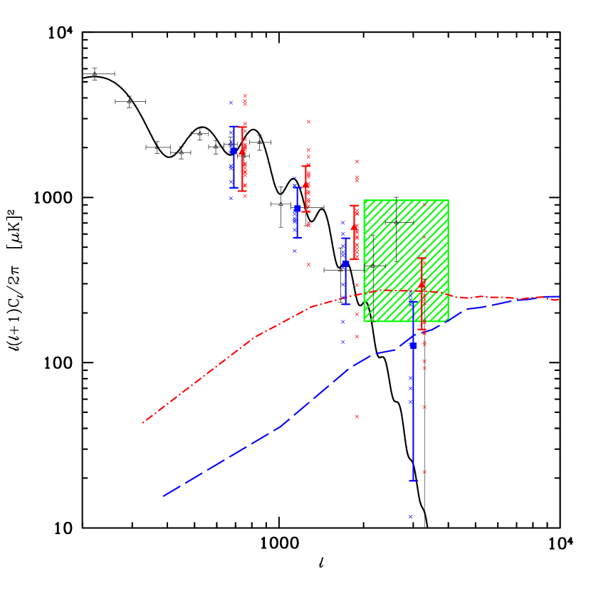
Figure 7.— Simulated observations of CMB plus SZ fields. The result of bandpower estimation on simulated observations of the $08^{\rm h}$ deep field containing noise, realizations of a fiducial $\Lambda$CDM model shown in black (solid line) and SZ foregrounds from the SPH and MMH $\sigma_{8}=1.0$ simulations. The blue (dashed) curve shows the average power spectrum of the input SPH maps and red (dash-dotted) is the average power spectrum of the input MMH maps. The red (triangle) points are the average bandpowers obtained from the analysis of 20 separate observations using the MMH maps. The blue (square) points are the average bandpower obtained from 10 SPH maps. The bandpower estimation pipeline recovers the correct power in the SZ dominated region $\ell>2000$. The green (shaded) rectangle shows the 95% confidence region for the high-$\ell$ CBI deep field result. Both the MMH and SPH codes show power consistent with the confidence region.

Results are shown in Fig. 7. The bandpowers are averaged over the 20 and 10 independent realizations from the two $\sigma_{8}=1.0$ simulations. The triangles (red) are for the MMH simulations and the SPH results are shown as squares (blue) points. The model used for the primary CMB contribution is also shown together with the $2\sigma$ confidence region for the deep excess. The errors shown are obtained from the variance of the measured bandpowers. The averages appear to recover the input power accurately in both regimes where either the primary CMB signal or SZ signal dominate.

The interpretation of the errors is of course complicated in the SZ-dominated regime by the non-Gaussianity of the SZ signal (eg. Zhang, Pen & Wang 2002). The small area considered in the simulations results in significant sample variance effects in the measurements of the SZ power. The scatter in the observed bandpowers over the different realizations is also shown in Fig. 7. The non-Gaussian scatter is significant, although this effect would decrease for the larger area probed in the joint three-field analysis and because the high-$\ell$ errors are dominated by the noise. It is also important to note that if the SZE is a significant source of the power in the observations, the sample variance component of the errors derived in the optimal spectrum estimation would be biased.

It is also interesting to note the effect of the low–$\ell$ contribution in the MMH simulations. There is a sizable contribution to the bandpowers below $\ell\sim 2000$. Although this effect may be due to the presence of one rather large cluster in the simulation, as discussed above, it raises the question of whether a SZ signal with high enough amplitude to explain the excess may already be constrained by its low–$\ell$ contributions.

5. Wiener-filtering the CBI Deep Field Observations

The CBI does not have sufficient frequency coverage to strongly distinguish different signals by their frequency dependence (e.g., CMB, SZ, and Galactic foregrounds). Spectral separation of the different components is therefore infeasible. Although the sensitivity of the CBI results presented here is not sufficient to conclusively identify individual features in the maps, we present examples and simulations of a Wiener-filtering technique described in Paper IV.

The total mode to mode correlations in the data are separated into four components in a typical analysis of the deep field visibilities with the weight matrix ${\bf W}$ as the sum

$${\bf W}=({\bf C}^{\rm N}+{\bf C}^{\rm CMB}+{\bf C}^{\rm SRC}+{\bf C}^{\rm res})^{-1},$$ (5)

with noise (N), CMB, known source (SRC) and residual source (res) components, respectively. (In papers II and III, the known source contribution is split into two components, for sources with and without measured flux densities.)

In the limit where all the components can be considered Gaussian random fields we can define the probability of each signal given the data as the Gaussian (Bond & Crittenden, 2002)

$$\ln P(\Delta^{\rm X}|\bar{\Delta}) = -\frac{1}{2}(\Delta^{\rm X}-\langle\Delta^{\rm X}|\bar{\Delta}\rangle)^{\dagger}({\bf C}^{\rm X})^{-1}(\Delta^{\rm X}-\langle\Delta^{\rm X}|\bar{\Delta}\rangle)$$ (6)

$$-\frac{1}{2}{\rm Tr}\ln{\bf C}^{\rm X}-N\ln\sqrt{2\pi},$$

where $\bar{\Delta}$ are the observations, $\Delta^{\rm X}$ is the map vector of the component ${\rm X}$, ${\bf C}^{\rm X}$ is the mode to mode correlation matrix for the component and $N$ is the number of modes in the map. The mean $\langle\Delta^{\rm X}|\bar{\Delta}\rangle$ defines the Wiener-filtered map of the component given the observations

$$\Delta^{\rm X}={\bf C}^{\rm X}{\bf W}\bar{\Delta},$$ (7)

with variance about the mean

$$\langle\delta\Delta^{\rm X}\delta\Delta^{{\rm X}\dagger}|\bar{\Delta}\rangle={\bf C}^{\rm X}-{\bf C}^{\rm X}{\bf W}{\bf C}^{\rm X}.$$ (8)

In our case, the maps $\Delta$ are column vectors containing the gridded visibility estimators (Paper IV), and sky plane maps can be obtained by Fast Fourier Transforming these estimators in the $uv$–plane. The correlation structure of the estimator grids are a necessary by-product of our gridding method and power spectrum estimation pipeline. The calculation of the correlations includes all the relevant information on the sampling structure and convolution of the fine-grained observation plane. Eq. 8 therefore includes all aspects of the uncertainties in the Wiener-filtered map resulting from the observations.

Due to the complex weighting applied to the observed visibilities in our gridding scheme it is difficult to assign units to the maps produced by simply Fourier transforming the gridded uv–plane. In order to obtain images with approximate normalizations in mJy/pixels, we reweight by dividing the vector at each lattice site by a second vector obtained by gridding a 1 mJy point source placed at the center of each field. It is important to note that this deconvolution is carried out in the coarse grained lattice and is not a full deconvolution of the effect of the dirty beam since no extra information is added to complete the uv–plane when gridding. In Fig. 8 we show the image obtained by Fourier transforming the gridded uv–plane of a simulated observation of a point source placed at the center of the $08^{\rm h}$ field.

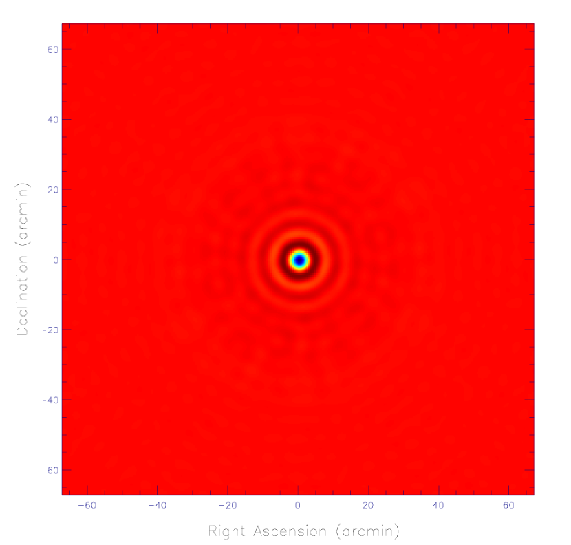
Figure 8.— The image produced by gridding a simulated observation of a point source placed at the center of the $08^{\rm h}$ field.

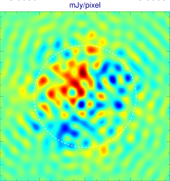
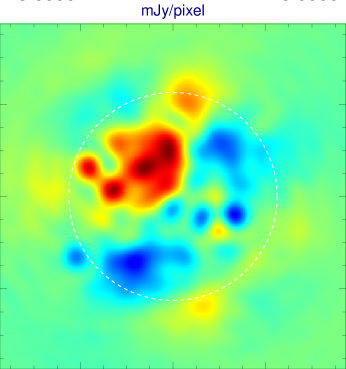
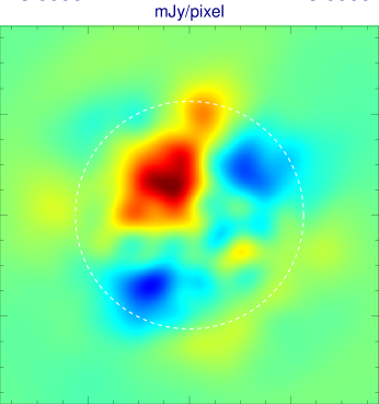
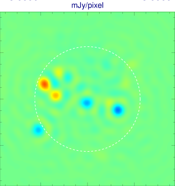
Figure 9.— Filtered images of the CBI $08^{\rm h}$ deep field. The total signal plus noise image (top left) displayed as a $70^{\prime}$ by $70^{\prime}$ field. The white (dashed) circle shows the $45^{\prime}$ FWHM of the primary beam. A total signal image (top right) is obtained by using the sum of CMB and point source foreground correlations as a template. The amplitude of the residual source background is set to a flux of $0.08{\rm Jy}^{2}{\rm sr}^{-1}$ in the filter. Using the joint deep field bandpowers as amplitudes in the filters we obtain the optimal image for the CMB (bottom left). This image encompasses the power attributed to the high-$\ell$ excess. The known point source residuals can also be filtered out of the data (bottom right). Colour scales are kept constant for the filtered images to ease comparison of the relative amplitudes of the components. The images are deconvolved by the response of a simulated source placed at the center of the field.

We show an example of the use of such filters in Fig. 9. The sequence shows the result of applying different filters to the $08^{\rm h}$ deep field observation. The original image (upper left) is first filtered to obtain a map of the total signal contributions which includes CMB and point sources (upper right). The CMB power spectrum obtained from the joint deep field analysis is then used as a template to obtain a map of the CMB contribution (lower left). The template includes the excess power above $\ell\sim 2000$. The post-subtraction residuals in the known point sources can also be separated into an image (lower right) which shows the total contribution of the modes which are projected out when estimating the power spectrum. The mean Wiener-filtered maps make no statement on the significance of any feature by themselves and considering only the mean can be misleading since there is no information on the allowed fluctuations around the mean in the map itself. This is particularly so in the case of interferometric observations where the nature of the noise and sampling uncertainties means that, although the power due to single features is conserved their structure in the sky plane is complicated by the extended nature of the correlations in the uncertainties. As shown above, however, in the Gaussian limit we can assign confidence limits on any features using Eq. 8.

A useful method of visualizing the significance of the features is by creating constrained realizations of the fluctuations and comparing these to the mean. For example we can obtain a random realization of the fluctuations by taking $\Delta_{i}^{\rm X}=({\bf C}^{\rm X}-{\bf C}^{\rm X}{\bf W}{\bf C}^{\rm X})^{1/2}\xi$ where $\xi$ are random Gaussian variates with unit norm. Adding these maps to the mean we get an idea of the allowed fluctuations about the mean. Strongly constrained features will be relatively unaffected by the fluctuations and represent the high signal–to–noise ratio limit where ${\bf C}^{\rm X}-{\bf C}^{\rm X}{\bf W}{\bf C}^{\rm X}\rightarrow 0$. Features measured at levels comparable to the ‘generalized’ noise of the observations will be washed out by the fluctuation levels and represent the limit ${\bf C}^{\rm X}-{\bf C}^{\rm X}{\bf W}{\bf C}^{\rm X}\rightarrow{\bf C}^{\rm X}$. The full pixel–pixel covariance matrix of the component map can be calculated by direct FFT of the covariance matrix or by taking Monte Carlo ensemble averages of the fluctuation realizations.

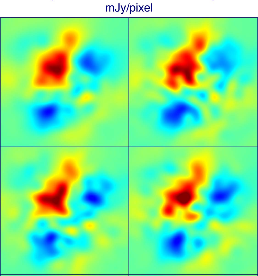
Figure 10.— Another way to illustrate whether the features seen in the Wiener-filtered images are robust is to show a few fluctuations about the mean (Wiener) map, here for the $08^{\rm h}$ deep field. The top left panel reproduces the mean CMB component map of Fig. 9. The remaining three panels show the addition of three constrained realizations of the allowed fluctuations to the mean map. At the signal–to–noise ratios of the larger scale CMB observations the features are robust to the fluctuations. Note that these images are ‘dirty maps’: no attempt has been made to compensate for gaps in the $uv$-coverage. The features are a combination of main-lobe and side-lobe responses to the CMB.

The level of fluctuations allowed around the mean for the CMB component of Fig. 9 is shown in Fig. 10. The four panel figure shows the Wiener filter of the component and the same map with three random realizations of the fluctuations added to it. As expected the CMB component is well constrained on the scales shown in the image since the signal–to–noise ratio is high: i.e. the main features in the map are stable with respect to the fluctuations. The features are therefore expected to be closely related to ‘real’ structures on the sky; but the nature of the observations, in particular the side-lobes of the point spread function (synthesized beam), means that the detailed structure of the features is not well constrained and most likely does not reflect the precise shape of the objects. The filtering of the large scale power by the interferometric observations also makes the correspondence with the large scale features on the sky not as intuitive as with sky plane based measurements.

Using the specific SZ models we introduced in § 4 we can now extend the image analysis by template-filtering the images specifically for SZ contributions. As described above the only components modeled in the total correlation matrix are the CMB, instrumental noise and source components. We therefore construct the SZ template as

$${\bf C}^{\rm SZ}=\sum_{B}{\cal C}^{\rm SZ}_{B}\frac{\partial{\bf C}^{\rm CMB}}{\partial{\cal C}_{B}}.$$ (9)

where the amplitudes ${\cal C}^{\rm SZ}_{B}$ are obtained by filtering the average SZ power spectra by the deep field band window functions (see Paper II).

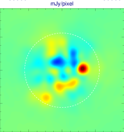
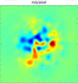
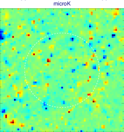
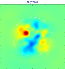
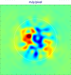
Figure 11.— Simulated observations of SZ signals. A single SZ realization is shown for the SPH (top left) and MMH (bottom left) simulations. The area represents a (lead-trail) differenced field used as the signal in a simulated observation of the $08^{\rm h}$ deep field. The maps are used to generate mock data sets with exact replications of the $uv$–coverage as the real data which are then filtered using the respective SZ templates. Mocks with close to negligible noise levels (top and bottom center) show the direct representation of the CBI processed input maps. The same realization but with the same noise levels as the observed data is in the top and bottom right panels. To within the accuracy allowed by the noise, the filtered images successfully reproduce the features of the input maps within the primary beam area.

The resulting SZ-filtered images should reproduce the structure in input SZ maps and we find that this is indeed the case. The sequence of images in Fig. 11 is an example of the filtering for one of the SPH maps (top row) and one of the MMH maps (bottom row). The left-hand panels show the input SZ maps (lead$-$trail) and the middle ones show the result of filtering mock data sets where the noise has been reduced to negligible levels. These provide a control set to compare with the reconstructed noisy observations shown on the right. The strongest features in both images reproduce the strongest SZ signatures in the input templates, although one has to take into account the tapering effect induced by the primary beam when comparing the input maps to the filtered data (see Paper IV). The tapering suppresses the amplitude of significant features further out in the beam with respect to those close to the center of the field. The noise level is such that the significance of the ‘detections’ is not obvious. These can be quantified by comparing with the allowed fluctuations about the mean Wiener filter (Eq. 8).

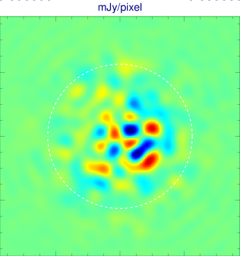
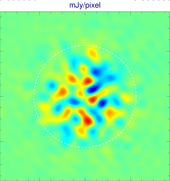
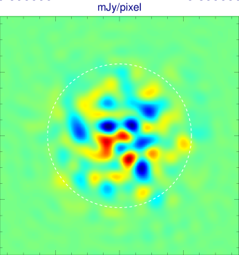
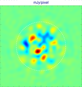
Figure 12.— The split deep data Wiener-filtered with the SZ template, for the $08^{\rm h}$ field (top) and the $20^{\rm h}$ field (bottom). There is no clear evidence of a high signal–to–noise stationary feature.

We have also applied the SZ Wiener filter to the deep field data itself. These SZ-filtered images scale linearly with the overall normalization of the SZ power spectrum. Hence, by calibrating the SZ template filters with the observed deep high–$\ell$ power, we can obtain an image with the same signal–to–noise ratio as the observations. In fig 12, we show the effect of the SZ filter on the data split in two roughly equal halves for the $08^{\rm h}$ and $20^{\rm h}$ deep field observations. When comparing the two halves the noise will be uncorrelated, so any commmon stationary signal of sufficient amplitude should appear in both halves. One sees no obvious strong signal-dominated stationary features, but there is one in each field, albeit with amplitudes comparable to the noise fluctuations. We conclude that the images are noise-dominated and there are no obvious features that could single–handedly account for the observed excess. This is in agreement with the excess being a statistical measurement as opposed to a high signal–to–noise observation.

6. Discussion

We have presented estimates for the possible contribution from the SZ effect to the CBI deep field observations which show evidence of an excess in power over standard primary CMB scenarios above $\ell\sim 2000$. Our numerical simulations show that an amplitude of $\sigma_{8}\approx 1$ appears to give, on average, enough power in the SZ signature to explain the excess. Current primary CMB and LSS data favor models with somewhat lower normalizations: for flat, HST–$h$ and LSS priors, $\sigma_{8}=0.88^{+0.08}_{-0.08}$ for the June 2002 dataset and $\sigma_{8}=0.86^{+0.04}_{-0.03}$ for the March 2003 compilation. Recent weak-lensing-only results, e.g., $0.83\pm 0.07$ (van Waerbeke et al., 2005), are also quite compatible with CMB-only values.

In assessing whether $\sigma_{8}\approx 0.9$ is too low to explain the anomaly, the non-Gaussian nature of the sample variance of the SZE should be included. This issue has been partially addressed in the literature (Cooray & Sheth, 2002; Springel, White & Hernquist, 2001; Komatsu & Seljak, 2002). Goldstein et al. (2003) have shown that a joint analysis of our CBI deep data with recent data from ACBAR (Kuo et al., 2004) and BIMA (Dawson et al., 2002) which simultaneously fits the amplitudes of the primary and SZ power spectra and roughly accounts for the non-Gaussianity of the SZE requires $\sigma_{8}=0.96^{+0.08}_{-0.16}$, with a maximum likelihood at 1.00, consistent with the constraints on $\sigma_{8}$ from primary CMB and LSS data, as illustrated in Figures 1 and 2. Readhead et al. (2004) applied a similar joint analysis to that in Goldstein et al. (2003) to the bandpowers of the ACBAR, BIMA, and CBI 2-year data. An attempt to bracket the effects of non-Gaussianity was made by allowing the sample-variance component of the error bar to increase by a factor of up to four: the estimate of $\sigma_{8}$ hardly changed, going from $0.98^{+0.06}_{-0.07}$ to $0.98^{+0.06}_{-0.08}$. Goldstein et al. (2003) used a factor of three to estimate the non-Gaussian effect. A bigger impact is found at the $2\sigma$ level: with a uniform prior in $\sigma_{8}$ there is a tail skewed to low $\sigma_{8}$, primarily because the amplitude being fit by the analysis is $\sigma_{8}^{7}$, and the distribution is roughly Gaussian in that variable, as shown explicitly in Fig. 12 of Readhead et al. (2004). We note that the errors are predominantly from noise and not sample-variance for the CBI data, which is why variation by a factor of four does not have a huge effect.

The Goldstein et al. (2003) and Readhead et al. (2004) analyses took into account the competing effects of the damping tail of the primary CMB fluctuations and the rising SZ power spectrum over the entire $\ell$ range, and not just in the $\ell>2000$ regime where the “excess” is clearly seen. The assumption is that the power spectra are described by an offset-log-normal distribution, which has been shown to hold well for Gaussian signals and noise (Bond, Jaffe & Knox, 2000; Sievers et al., 2003). The distribution becomes a Gaussian one in the noise-dominated regime and a log-normal one in the signal-dominated regime. If the signal comes from clusters and groups, the latter will not be accurate, and further work is needed to properly assess the limits derived from the “excess”. What is needed is a full suite of simulations, guided by semi-analytic theory, to Monte Carlo the effects of non-Gaussianity rather than rely on expanded signal-errors.

The excellent agreement among the runs using the two separate hydrodynamic algorithms is encouraging and lends support to the conclusions on the required normalization. We note that the simulations employed in this work were developed and run independently from each other and the CBI analysis effort (Bond et al., 2002; Zhang, Pen & Wang, 2002). However, both simulations were adiabatic, with entropy increases occurring only by shock heating. The influence of cooling and entropy injection from supernovae, etc., on the predicted SZ spectrum remains to be explored, as does the effect of such technical issues as numerical convergence as the simulation resolution is changed.

The limited number of mock simulations we have carried out show that our experimental setup does reproduce correctly the signal of simulated SZ foregrounds. This suggests the Gaussian assumption implicit in our bandpower estimation procedures does not break down at the SZ signal-to-noise ratios of the deep field observations.

If the excess is not due to the SZE, what could it be? Other possible origins of the excess were addressed in Paper II. It is inconsistent with adiabatic inflationary predictions for primary anisotropies on the damping tail only at the $\sim 3\sigma$ level. The excess clearly needs to be further explored, both within the CBI dataset itself, and also by correlating with other observations of these deep fields. The statistical nature of the detected excess means we cannot identify single features responsible for the excess in the deep fields even after Wiener-filtering the data with SZ derived templates.

Our principal conclusion is that the CBI excess could be a result of the SZ effect for the class of $\Lambda$CDM concordance models if $\sigma_{8}$ is in the upper range of values allowed by current CMB data. The simple ${\cal C}_{\ell}\propto\sigma_{8}^{7}(\Omega_{b}h)^{2}$ scaling (eq. 2) shows that the lower $\sigma_{8}$ values preferred by the CMB data imply SZ signals below, but not too far below, the sensitivity obtained by the CBI deep observations. This work also highlights how the signature of the SZ effect has great potential for constraining the amplitude $\sigma_{8}$. The sensitive scaling of the CMB power with $\sigma_{8}$ will result in significant constraints even with large errors on the observed bandpowers. This further underlines the significance of ‘blank field’ observations at $\ell\gtrsim 2000$ which should reveal the SZ structure that necessarily lurks as a byproduct of CMB-normalized structure formation models.

References

- Allen et al. (2003) Allen, S.W. Schmidt, R.W. Fabian, A.C. & Ebeling, H. 2003, MNRAS 342, 287 (astro-ph/0208394)
- Atrio-Barandela & Mucket (1999) Atrio-Barandela, F. & Mucket, J., 1999, ApJ, 515, 465
- Bacon et al. (2002) Bacon, D., Massey, R., Refregier, A., & Ellis, R. 2002, MNRAS, 344, 673 (astro-ph/0203134)
- Bardeen, Bond, Kaiser, & Szalay (1986) Bardeen, J. M., Bond, J. R., Kaiser, N., & Szalay, A. S. 1986, ApJ, 304, 15
- Bennett et al. (1996) Bennett, C. L. et al. 1996, ApJ, 464, L1
- Birkinshaw, Gull & Hardebeck (1984) Birkinshaw, M., Gull, S. F., Hardebeck, H. 1984, Nature, 309, 34
- Bond (1988) Bond, J. R. 1988, in The Early Universe, p. 283-334, ed. W. Unruh and G. Semenoff, Dordrecht:Reidel.
- Bond (1994) Bond, J. R. 1994, in Relativistic Cosmology, ed., M. Sasaki, Proc. 8th Nishinomiya-Yukawa Memorial Symposium (Universal Academy Press), pp. 23-55, (astro-ph/9406075)
- Bond (1996) Bond, J. R. 1996, in Cosmology and Large Scale Structure, Les Houches Session LX, (ed. R. Schaeffer, J. Silk, M. Spiro & J. Zinn-Justin), pp. 469-674. Elsevier. (Available at http://www.cita.utoronto.ca/bond/papers/houches/)
- Bond & Crittenden (2002) Bond, J. R. & Crittenden, R. G., 2002, in Structure Formation in the Universe, 241-280, R.G. Crittenden and N.G. Turok, eds., Proc. NATO ASI (Kluwer Academic Publishers) (astro-ph/0108204)
- Bond & Efstathiou (1987) Bond, J. R. & Efstathiou, G. 1987, MNRAS, 226, 655
- Bond & Jaffe (1999) Bond, J. R. & Jaffe, A. H. 1999, Large-Scale Structure in the Universe, Phil. Trans. R. Soc. Lond. A 357, 57 ( astro-ph/9809043)
- Bond, Jaffe & Knox (2000) Bond, J. R., Jaffe, A. H., & Knox, L. 2000, ApJ, 533, 19
- Bond et al. (1998) Bond, J. R., Kofman, L., Pogosyan, D. & Wadsley, J. 1998, in Wide Field Surveys in Cosmology, Proc. XIV IAP Colloquium, p. 17, (ed, Colombi, S. & Mellier, Y.), Paris: Editions Frontieres (astro-ph/9810093)
- Bond & Myers (1996) Bond, J. R. & Myers, S. 1996, ApJS, 103, 1
- Bond et al. (2002) Bond, J. R., Ruetalo, M. I., Wadsley, J. W. & Gladders, M. D., 2002, Astron. Soc. Pacific Conference Series 257, 327-339, AMiBA 2001: High-z Clusters, Missing Baryons, and CMB Polarization, Proc. TAW8, Taiwan, June, ed. L-W Chen, C-P Ma, K-W Ng and U-L Pen, (San Francisco: Astron. Soc. Pacific) (astro-ph/0112499)
- Bond et al. (2003) Bond, J. R., Contaldi, C. R. & Pogosyan, D. 2003, Phil. Trans. R. Soc. Lond. A 361, 2435 (astro-ph/0310735)
- Borgani et al. (2001) Borgani, S., et al. 2001, ApJ, 561, 13 (astro-ph/0106428)
- Brown et al. (2003) Brown, M., Taylor A., Bacon D., Gray M., Dye S., Meisenheimer K. & Wolf C. 2003, MNRAS, 341, 100 (astro-ph/0210213)
- Carlberg et al. (1997) Carlberg, R. G., Morris, S. L., Yee, H. K. C., Ellingson, E. 1997, ApJ, 479, L19
- Carlstrom et al. (1996) Carlstrom, J. E. et al. 1996, ApJ, 456, L75
- Cole & Kaiser (1988) Cole, S. & Kaiser, N., 1988, MNRAS, 233, 637
- Cooray (2000) Cooray, A., 2000, Phys. Rev. D, 62, 103506
- Cooray & Sheth (2002) Cooray, A. & Sheth, R. 2002, Physics Reports 372, 1
- Dawson et al. (2002) Dawson, K.S., Holzapfel, W.L., Carlstrom, J.E., LaRoque, S.J., Miller, A., Nagai, D. & Joy, M. 2002, ApJ 581, 86 (astro-ph/0206012)
- Dodelson et al. (2001) Dodelson, S., et al. 2001, ApJ, 572, 140 (astro-ph/0107421)
- Efstathiou et al. (1992) Efstathiou, G., Bond, J. R. & White, S. D. M. 1992, MNRAS, 258, 1P
- Eke et al. (1996) Eke, V. R., Cole, S., Frenk, C. S. 1996, MNRAS, 282, 263
- Fan & Bahcall (1998) Fan, X. & Bahcall, N. A. 1998, ApJ, 504, 1
- Goldstein et al. (2003) Goldstein J., et al. 2003, ApJ, 599, 773 (astro-ph/0212517)
- Grainge et al. (2002) Grainge, K., et al. 2002, MNRAS, 329, 890
- Grainge et al. (2003) Grainge, K., et al. 2003, MNRAS, 341, L23
- Halverson et al. (2001) Halverson, N. W. et al. 2002, ApJ, 568, 38
- Hamana et al. (2003) Hamana, T. et al. 2003, ApJ, 597, 98 (astro-ph/0210450)
- Heymans et al. (2004) Heymans, C., Brown, M. Heavens, A., Meisenheimer, K. & Taylor, A. & Wolf, C. 2004, MNRAS, 347, 895 (astro-ph/0310174)
- Holzapfel et al. (1997) Holzapfel, W. L. et al. 1997, ApJ, 479, 17
- Hoekstra et al. (2002) Hoekstra, H., Yee, H. K. C. & Gladders, M. D. 2002, ApJ, 577, 595 (astro-ph/0204295)
- Jaffe et al. (2001) Jaffe, A. H. et al. 2001, Phys. Rev. Lett., 86, 3475
- Jarvis et al. (2003) Jarvis, M., Bernstein, G., Fischer, P., Smith, D., Jain, B., Tyson, A. & Wittman, D., 2003, AJ, 1025, 1014
- Kogut et al. (2003) Kogut, A. et al., 2003, ApJS, 148, 161
- Komatsu & Kitayama (1999) Komatsu, E. & Kitayama, T., 1999, ApJ, 526, L1
- Komatsu & Seljak (2002) Komatsu, E. & Seljak, U. 2002, MNRAS, 336, 1256 (astro-ph/0205468)
- Kuo et al. (2004) Kuo, C. L. et al., 2004, ApJ, 600, 32 (astro-ph/0212289)
- Lahav et al. (2002) Lahav, O., et al. 2002, MNRAS, 333, 961 (astro-ph/0112162)
- Lange et al. (2001) Lange, A. E., et al. 2001, Phys. Rev. D, 63, 042001
- Lee et al. (2001) Lee, A. T., et al. 2001, ApJ, 561, L1
- Makino & Suto (1993) Makino, N., & Suto, Y. 1993, ApJ, 405, 1
- Mason, Myers, & Readhead (2001) Mason, B. S., Myers, S. T., & Readhead, A. C. S. 2001, ApJ, 555, L11
- Mason et al. (2003) Mason, B. S., et al. 2003, ApJ, 591, 540 (Paper II)
- Mauskopf et al. (2000) Mauskopf, P. D., et al. 2000, ApJ, 536, L59
- Melchiorri & Silk (2002) Melchiorri, A. & Silk, J., 2002 Phys. Rev. D 66, 041301 (astro-ph/0203200)
- Miller et al. (1999) Miller, A. D., et al. 1999, ApJ, 524, L1
- Mo & White (1996) Mo, H. J. & White, D. M., 1996, MNRAS, 282, 347
- Molnar & Birkinshaw (2000) Molnar, S. & Birkinshaw, 2000, ApJ, 537, 542
- Myers et al. (2003) Myers, S. T. et al. 2003, ApJ, 591, 575 (Paper IV)
- Netterfield et al. (2002) Netterfield, C. B., et al. 2002, ApJ 571, 604 (astro-ph/0104460)
- Padin et al. (2001) Padin, S., et al. 2001, ApJ, 549, L1 (Paper I)
- Peacock & Dodds (1994) Peacock, J. A. & Dodds, S. J. 1994, MNRAS, 267, 1020
- Peacock et al. (2001) Peacock, J. A., et al. 2001, Nature, 410, 169
- Pearson et al. (2003) Pearson, T. J., et al. 2003, ApJ, 591, 556 (Paper III)
- Peebles & Yu (1970) Peebles, P. J. E. & Yu, J. T. 1970, ApJ, 162, 815
- Pen (1998a) Pen, U.-L., 1998a, ApJS, 115, 19
- Pen (1998b) Pen, U.-L., 1998b, ApJ, 498, 60
- Pen (1998c) Pen, U.-L. 1998c, ApJ, 504, 60
- Pierpaoli, Scott & White (2001) Pierpaoli, E., Scott, D., & White, M. 2001, MNRAS, 325, 77
- Pierpaoli et al. (2003) Pierpaoli, E., Borgani, S., Scott, D., & White, M. 2003, MNRAS, 342, 163 (astro-ph/0210567)
- Press & Schechter (1974) Press, W. H. & Schechter, P. 1974, ApJ, 187, 425
- Pryke et al. (2002) Pryke, C., Halverson, N. W., Leitch, E. M., Kovac, J., Carlstrom, J. E., Holzapfel, W. L., & Dragovan, M. 2002, ApJ, 568, 46
- Readhead et al. (2004) Readhead, A. C. R., et al. 2004, ApJ, 609, 498
- Refregier et al. (2002) Refregier, A., Rhodes, J., & Groth, E. J. 2002, ApJ, 572, L131 (astro-ph/0203131)
- Reiprich & Böhringer (2002) Reiprich, T. H. & Böhringer, H. 2002, ApJ, 567, 716 (astro-ph/0111285)
- Ruhl et al. (2003) Ruhl, J.E. et al., 2003, ApJ, 599, 786 (astro-ph/0212229)
- Schuecker et al. (2003) Schuecker P., Bohringer H., Collins C.A & Guzzo L. 2003, A&A, 398, 867 (astro-ph/0208251)
- Scott et al. (2002) Scott, P.F. et al. 2002, MNRAS 341, 1076 (astro-ph/0205380)
- Seljak (2002) Seljak, U. 2002, MNRAS, 337, 769 (astro-ph/0111362)
- Seljak, Burwell & Pen (2001) Seljak, U., Burwell, J. & Pen, U.-L., 2001, Phys. Rev. D, 63, 063001
- Sievers et al. (2003) Sievers, J. L., et al. 2003, ApJ, 591, 599 (Paper V)
- Silk (1968) Silk, J. 1968, ApJ, 151, 459
- Spergel et al. (2003) Spergel, D. N., et al., 2003, ApJS, 148, 175
- Springel, White & Hernquist (2001) Springel, V., White, M., & Hernquist, L. 2001, ApJ, 549, 681, erratum; Springel, V., White, M., & Hernquist, L. 2001, ApJ, 562, 1086
- Sugiyama (1995) Sugiyama, N. 1995, ApJS. 100, 281
- Sunyaev & Zeldovich (1970) Sunyaev, R. A. & Zeldovich, Ya. B. 1970, Ap&SS, 7, 3
- Szalay et al. (2001) Szalay, A. S. et al. 2001 , ApJ, 591, 1 (astro-ph/0107419)
- Udomprasert et al. (2004) Udomprasert, P. S., Mason, B. S., Readhead, A. C. S., & Pearson, T. J. 2004, ApJ, 615, 63
- Verde et al. (2002) Verde, L. et al. 2002, MNRAS, 335, 432 (astro-ph/0112161)
- Viana, Nichol & Liddle (2001) Viana, P. T .P., Nichol, R. C. & Liddle, A. R. 2001, ApJ, 569, L75 (astro-ph/0111394)
- Voevodkin & Vikhlinin (2004) Voevodkin, A. & Vikhlinin, A. 2004, ApJ, 601, 610 (astro-ph/030554)
- Wadsley, Stadel & Quinn (2003) Wadsley, J. W., Stadel, J. & Quinn, T. 2003, New Astronomy, 9, 137
- van Waerbeke et al. (2002) van Waerbeke, L., Mellier, Y., Pello, R., Pen, U.-L, McCracken, H. J., & Jain, B. 2002, A&A, 393, 369 (astro-ph/0202503)
- van Waerbeke et al. (2005) van Waerbeke, L., Mellier, Y., & Hoekstra, H. 2005, A&A, 429, 75
- Zhang & Pen (2001) Zhang, P. J., & Pen, U.-L., 2001, ApJ, 549, 18
- Zhang, Pen & Wang (2002) Zhang, P. J., Pen, U.-L. & Wang, B. 2002, ApJ, 577, 555 (astro-ph/0201375)