Cosmological Parameters from Cosmic Background Imager Observations and Comparisons with BOOMERANG, DASI, and MAXIMA

Abstract

We report on the cosmological parameters derived from observations with the Cosmic Background Imager (CBI), covering 40 square degrees and the multipole range $300\lesssim\ell\lesssim 3500$. The angular scales probed by the CBI correspond to structures which cover the mass range from $10^{14}M_{\sun}$ to $10^{17}M_{\sun}$, and the observations reveal, for the first time, the seeds that gave rise to clusters of galaxies. These unique, high-resolution observations also show damping in the power spectrum to $\ell\sim 2000$, which we interpret as due to the finite width of the photon-baryon decoupling region and the viscosity operating at decoupling. Because the observations extend to much higher $\ell$ the CBI results provide information complementary to that probed by the BOOMERANG, DASI, MAXIMA, and VSA experiments. When the CBI observations are used in combination with those from COBE-DMR  we find evidence for a flat universe, $\Omega_{\rm tot}=1.00_{-0.12}^{+0.11}$ (1-$\sigma$), a power law index of primordial fluctuations, $n_{s}=1.08_{-0.10}^{+0.11}$, and densities in cold dark matter, $\Omega_{\rm cdm}h^{2}=0.16_{-0.07}^{+0.08}$, and baryons, $\Omega_{b}h^{2}=0.023_{-0.010}^{+0.016}$. With the addition of large scale structure priors the $\Omega_{\rm cdm}h^{2}$ value is sharpened to $0.10_{-0.03}^{+0.04}$, and we find $\Omega_{\Lambda}=0.67_{-0.13}^{+0.10}$. In the $\ell<1000$ overlap region with the BOOMERANG, DASI, MAXIMA, and VSA experiments, the agreement between these four experiments is excellent, and we construct optimal power spectra in the CBI bands which demonstrate this agreement. We derive cosmological parameters for the combined CMB experiments and show that these parameter determinations are stable as we progress from the weak priors using only CMB observations and very broad restrictions on cosmic parameters, through the addition of information from large scale structure surveys, Hubble parameter determinations and Supernova-1a results. The combination of these with CMB observations gives a vacuum energy estimate of $\Omega_{\Lambda}=0.70_{-0.05}^{+0.05}$, a Hubble parameter $h=0.69\pm 0.04$ and a cosmological age of $13.7\pm 0.2$ Gyr. As the observations are pushed to higher multipoles no anomalies relative to standard models appear, and extremely good consistency is found between the cosmological parameters derived for the CBI observations over the range $610<\ell<2000$ and observations at lower $\ell$.

1. Introduction

The angular power spectrum of the Cosmic Microwave Background (CMB) has emerged as a major arena in which our cosmological models and theories of cosmic structure formation can be tested. In this paper we estimate cosmological parameters from observed power spectra from the Cosmic Background Imager (CBI) and the low $\ell$ anchor of the COBE-DMR observations, and we relate the CBI observations to BOOMERANG, DASI, MAXIMA, and earlier CMB experiments. We have also incorporated results from the VSA (Scott et al., 2002) which were reported at the same time as these CBI results. We also use results from large scale structure studies (LSS), supernova observations (SN1a), and Hubble constant (HST-$h$) measurements to refine estimates of key cosmological parameters, both for CBI+DMR alone, and for the CBI results in combination with other CMB observations.

During the year 2000 observing season, the CBI covered three deep fields of diameter roughly $1^{\circ}$ (Mason et al., 2003, hereafter Paper II), and three mosaic regions, each of size roughly 13 square degrees (Pearson et al., 2003, hereafter Paper III). Methods used for power spectrum estimation from these interferometry observations are described in Myers et al. (2003, hereafter Paper IV). The results from the 2001 observing season, when combined with the observations from 2000, will extend the mosaics to 80 square degrees, roughly doubling the amount of mosaic data. This will improve upon the parameter estimates given here but has yet to be analyzed.

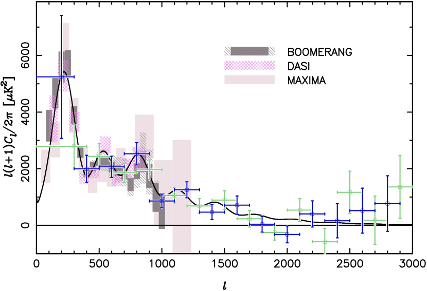
Figure 1.— Features in the anisotropy spectrum (from Paper III). The first acoustic peak is seen at high sensitivity in the BOOMERANG (Netterfield et al., 2002), DASI (Halverson et al., 2002), and MAXIMA (Lee et al., 2001) observations, while the second and third acoustic peaks are seen at lower sensitivity (the rectangles indicate the 68% confidence intervals on band-power). The circles (dark blue) and squares (green) show the odd and even binnings of the CBI results from the joint spectrum of the three mosaic fields (see Paper III. Note that the two binnings are highly correlated with each other and are not independent measurements of the power spectrum). The damping tail is clearly seen in the CBI spectrum, and, in the region of overlap, all four experiments are in excellent agreement, as is discussed in § 5.2. The black curve is the joint model also discussed in § 5.2.

Over the past several years, as the CMB observations have improved, the basic ${\cal C}_{\ell}$ features predicted in the eighties for inflation-motivated models in which cosmic structure arises from Gaussian-distributed curvature fluctuations (e.g., Bond & Efstathiou 1987) have emerged: (1) A “Sachs-Wolfe” plateau at low multipole moments, seen by COBE-DMR (Bennett, 1996) and other large angle experiments. This probes the gravitational potentials at the last scattering surface and along the line of sight on scales that were not in causal contact at the epoch of photon decoupling at redshift $z\sim 1100$. (2) The long-sought first acoustic peak at $\ell\sim 200$, tentatively first seen by combining results from a heterogeneous mix of CMB results (e.g., Bond, Jaffe & Knox, 2000), then in single experiments, TOCO (Miller et al., 1999) and BOOMERANG-NA North American Test Flight (Mauskopf et al., 2000). This was followed shortly after by the spectacularly detailed first peak mapping by the BOOMERANG Antarctic flight (de Bernardis et al., 2000; Netterfield et al., 2002) and MAXIMA (Hanany et al., 2001; Lee et al., 2001); (3) and the detection of the next few peaks and dips by BOOMERANG (Netterfield et al., 2002; de Bernardis et al., 2002) and DASI (Halverson et al., 2002). Observations from the more recent experiments are shown in Figure 1. Following these successes, three other key ingredients remained to be demonstrated (see, e.g., Bond 1996 for a review): (4) The peaks and dips continue to higher $\ell$ at ever diminishing amplitude, in a damping tail directly tied to the viscosity in the photon-baryon fluid as they decouple, and to the finite width of that decoupling region. (5) A necessary and highly predictable linear polarization power spectrum, fed by the polarization-dependent Thomson scattering of the primary CMB anisotropy developed during photon break-out from the decoupling region. (6) Secondary anisotropies that are an inevitable consequence as waves develop nonlinearly, breaking to form collapsed structures.

The CBI power spectra show clear evidence for a decline consistent with the damping tail (4), as can be seen in Figure 1. The Sunyaev-Zeldovich effect has of course been observed in clusters of galaxies at very high sensitivities, so (6) is there, and there may be evidence of a statistical SZE signal from distant clusters in the CBI deep field observations (Papers II and VI), but further experimental verification is needed. We address some issues associated with (4) and (6) in this paper, and (6) is treated in more detail in Bond et al. (2003, hereafter Paper VI). There are many experiments underway to address (5) and the first detection of polarization in the microwave background has recently been announced Leitch et al. (2002); Kovac et al. (2002); CBI has been observing polarization since September 2002. A longer term possibility would provide a 7th pillar, the detection of a component attributable to gravity waves in the CMB observations. However, unlike the other six items, inflation models differ substantially in the amount of gravity waves predicted, with very small undetectable imprints on the CMB being quite feasible.

One reason that theory can be so definitive is that the primary CMB anisotropies probe the linear regime of fluctuations and can be calculated in exquisite detail. The adiabatic inflation-motivated paradigm continues to do remarkably well as our knowledge of ${\cal C}_{\ell}$ and other parameters improves. Just as powerful though is the large reduction in the space of possible theories which accurate measurements of the anisotropies provide. The positioning of the peaks is a strong argument in favor of predominantly curvature (adiabatic) fluctuations as opposed to isocurvature ones. In addition the multiple peaks are a strong argument in favour of coherent (passive) perturbations as opposed to incoherent (active) ones, e.g., those associated with cosmic defect theories of structure formation (Allen et al., 1997; Turok, Pen, & Seljak, 1998; Contaldi, Hindmarsh, & Magueijo, 1999).

Minimal inflation-based models characterize the predictions with a handful of cosmological parameters $\{\Omega_{\rm{tot}}$, $\Omega_{\Lambda}$, $\Omega_{b}h^{2}$, $\Omega_{\rm cdm}h^{2}$, $n_{s}$, $\tau_{C}$, $\ln{\cal C}_{10}\}$. These are now very familiar to astrophysicists (see, e.g., Bond, Efstathiou & Tegmark, 1997; Lange et al., 2001; Jaffe et al., 2001; Pryke et al., 2002; Netterfield et al., 2002). The present-day density $\rho_{j}$ of a component $j$ is $\Omega_{j}=8\pi G\rho_{j}/(3H_{0}^{2})$ where $H_{0}=100h\;$km s^-1 Mpc^-1 is the Hubble constant. We use the notation $\omega_{j}\equiv\Omega_{j}h^{2}$ for the related physical density, which is more relevant for the CMB. We therefore consider the densities of baryons, $\omega_{b}$, and of cold dark matter (CDM), $\omega_{\rm cdm}$, with total matter density parameter $\Omega_{m}=\Omega_{\rm cdm}+\Omega_{b}$. The energy density parameter associated with a cosmological constant is $\Omega_{\Lambda}$ and the total density is $\Omega_{\rm{tot}}=\Omega_{m}+\Omega_{\Lambda}$, related to the curvature energy density parameter by $\Omega_{k}=1-\Omega_{\rm{tot}}$. The initial spectrum of density perturbations is described by an amplitude, which we usually take to be a factor $\mathcal{C}_{10}$ multiplying the CMB spectrum, and the spectral tilt of scalar (density) perturbations, $n_{s}$ (defined so that the initial three-dimensional perturbation power in gravitational potential fluctuations per $\ln k$ is $\propto k^{n_{s}-1}$, with $n_{s}=1$ thus giving a scale invariant spectrum). We also consider the Thomson depth $\tau_{C}$ to the epoch of reionization, presumably associated with luminous star formation in the earliest forming dwarf galaxies. Many more parameters may be needed to completely describe inflationary models. These include the gravity-wave induced tensor amplitude and tilt, variations of tilt with wavenumber, relativistic particle densities, more complex dynamics associated with the dark energy $\Omega_{\Lambda}$, etc. We discuss these briefly below, but concentrate on the minimal set of 7 parameters for this paper. The grid of parameter values we have used in this work is an extended version of the one used by Lange et al. (2001), and is reproduced in Table 1.

Table 1Parameter Grid for Likelihood Analysis

Parameter	Grid:
$\Omega_{k}$	0.9	0.7	0.5	0.3	0.2	0.15	0.1	0.05	0	-0.05	-0.1	-0.15
	-0.2	-0.3	-0.5
$\omega_{\rm cdm}$	0.03	0.06	0.08	0.10	0.12	0.14	0.17	0.22	0.27	0.33	0.40	0.55	0.8
$\omega_{b}$	0.003125	0.00625	0.0125	0.0175	0.020	0.0225	0.025	0.030	0.035	0.04	0.05	0.075
	0.10	0.15	0.2
$\Omega_{\Lambda}$	0	0.1	0.2	0.3	0.4	0.5	0.6	0.7	0.8	0.9	1.0	1.1
$n_{s}$	1.5	1.45	1.4	1.35	1.3	1.25	1.2	1.175	1.15	1.125	1.1
	1.075	1.05	1.025	1.0	0.975	0.95	0.925	0.9	0.875	0.85	0.825
	0.8	0.775	0.75	0.725	0.7	0.65	0.6	0.55	0.5
$\tau_{c}$	0	0.025	0.05	0.075	0.1	0.15	0.2	0.3	0.4	0.5	0.7

The main target of the CBI, as with most other experiments to date, is to measure primary anisotropies of the CMB, those which can be calculated using linear perturbation theory. The maps shown in Papers III and VI are, to a first approximation, images of damped sound wave patterns that existed about 400,000 years after the Big Bang at a time when the photons were freed from the plasma. However, the images are actually a projected mixture of dominant and subdominant physical processes occurring through the photon decoupling “surface”, a fuzzy wall at redshift $z_{\rm dec}\sim 1050$, when the Universe passed from optically thick to thin to Thomson scattering over a comoving distance $\sim 7\,\omega_{m}^{-1/2}\,{\rm Mpc}$. (Specific numbers here are appropriate for a $\Lambda$CDM universe preferred by the parameter estimates in this paper; $\omega_{m}\sim 0.14$ is one of our conclusions.) Prior to this epoch, acoustic wave patterns in the tightly-coupled photon-baryon fluid on scales below the comoving “sound crossing distance” at decoupling, $\sim 50\,\omega_{m}^{-1/2}\,{\rm Mpc}$ (i.e., $\sim 50\,\omega_{m}^{-1/2}\,{\rm kpc}$ physical), were viscously damped and strongly so on scales below the damping scale $\sim 4\,\omega_{m}^{-1/2}\,{\rm Mpc}$. This is closely related to the thickness over which decoupling occurred. Subsequently, the photons freely-streamed along geodesics to us, mapping (through the angular diameter distance relation) the post-decoupling spatial structures in the temperature to the angular patterns we observe now as the primary CMB anisotropies. For example, the sound crossing and damping scales translate to multipoles $\sim 110$ and $\sim 1300$, respectively. Free-streaming along our (linearly perturbed) past light cone leaves the pattern largely unaffected, except for the effect of temporal evolution in the gravitational potential wells as the photons propagate through them which leaves a further $\Delta T$ imprint, known as the integrated Sachs-Wolfe effect.

A number of effects complicate this simple picture of direct mapping of acoustic compression and rarefaction regions: anisotropies are also fed by the electron flow at decoupling leading to a Doppler effect, the changing gravitational potential as the universe passes from domination by relativistic to nonrelativistic species and small terms associated with polarization. The damping is of course a major radiative transfer problem, connecting the tightly-coupled baryon-photon fluid regime when shear viscosity and thermal conduction accurately describe the damping through to the free-streaming regime when full transport is needed. Intense theoretical work over three decades has put accurate calculations of this linear cosmological radiative transfer problem on a firm footing. We discuss this further in § 7.

Of course there are a number of nonlinear effects that are also present in the maps. These secondary anisotropies include weak-lensing by intervening mass, Thomson-scattering by the nonlinear flowing gas once it became “reionized” at $z\sim 10$–$20$, the thermal and kinematic SZ effects, and the red-shifted emission from dusty galaxies. They all leave non-Gaussian imprints on the CMB sky. Theoretical predictions based on the best-fit models suggest that for CBI, only the thermal SZ effect would be within striking distance. This effect is addressed in Paper VI.

The structure of the paper is as follows. In § 2 we first summarize the various priors from non-CMB observations that we use when estimating cosmological parameters. In § 3 and Appendix A, we describe the methods we have used for parameter determination from power spectrum estimates, and the tests we have performed to demonstrate accuracy. We obtain estimates for our minimal inflation-based parameter set in § 4, and also apply the techniques of Appendix A to determine optimal bandpower spectra in § 5. We check for consistency between the mosaic and deep field results by comparing optimally calculated spectra for various subsets of the data. In the parameter estimations we restrict ourselves to the $\ell<2000$ region. The spectrum at $\ell>2000$ is discussed in Paper VI together with the level of secondary anisotropy expected from the Sunyaev-Zeldovich effect in that regime, and whether this is the origin of the excess power seen in the CBI observations at high $\ell$. In § 5 we compare our results with those of other CMB experiments as a further consistency check. We then combine all available results with the CBI observations to obtain an all inclusive set of parameter estimates in § 6. In § 7 we summarize the physical effects probed directly by the CBI observations. Our conclusions are presented in § 8.

2. Prior Probabilities Used in Cosmological Parameter Extraction

We apply a sequence of increasingly strong “prior” probabilities successively to the likelihood functions. These are well known from the CMB literature (e.g., Bond & Jaffe, 1998; Lange et al., 2001; Jaffe et al., 2001; Netterfield et al., 2002). The priors we apply are listed below.

1) The “weak-$h$” prior: this prior restricts the Hubble parameter to $0.45<h<0.9$, and also imposes an age restriction, $t_{0}>10$ Gyr, and a restriction on the matter density, $\Omega_{m}>0.1$. These are all weak priors that most cosmologists would readily agree on.

2) The “flat” prior: as we shall see, the CBI observations strongly support $\Omega_{k}\approx 0$, so the addition of a flat prior to weak-$h$ seems reasonable. This is especially so if the target is parameters associated with inflation models. Although it is possible for inflation models to give large mean curvature with non-negligible $|\Omega_{k}|$, they are rather baroque.

3) The “LSS” prior: The LSS prior we use here is slightly modified over that used earlier (Bond & Jaffe, 1998; Lange et al., 2001; Jaffe et al., 2001; Netterfield et al., 2002) and is described in detail in Paper VI. It involves a constraint on the amplitude $\sigma_{8}^{2}$ and shape $\Gamma_{\rm eff}$ of the (linear) density power spectrum. Here $\sigma_{8}$ is the rms density power on scales corresponding to rich clusters of galaxies ($8\,h^{-1}\,{\rm Mpc}$) and $\Gamma_{\rm eff}$ mainly parameterizes the critical length scale when the universe passed from dominance by relativistic matter to dominance by non-relativistic matter. Both constraints depend upon our basic minimal parameter set in complex ways. The distributions in both these LSS parameters are taken to be quite broad, akin to a “weak LSS prior”. We take a distribution for the combination $\sigma_{8}\Omega_{m}^{0.56}$ which is a Gaussian (first error) smeared by a uniform (top-hat) distribution (second error): $0.47^{+.02,+.11}_{-.02,-.08}$. The 0.47 value is about 15% below the value adopted in the earlier CMB papers, as discussed in Paper VI, but the distribution shape is the same. To use it, the relation between ${\cal C}_{10}$ and $\sigma_{8}^{2}$ is needed for each cosmological model considered. For the shape prior, we make use of the similarity, over the wavenumber band that most large scale structure data probes, between changes in the spectral index $n_{s}$ and changes in the shape parameter $\Gamma\approx\Omega_{m}h\,\exp[-\Omega_{B}(1+\Omega_{m}^{-1}(2{h})^{1/2})]$. The latter includes a strong dependence upon $\Omega_{m}h$ as well as a rough $\Omega_{B}$ modification. We combine the two dependences into a single constraint on the parameter $\Gamma_{\rm eff}$ = $\Gamma+(n_{s}-1)/2$ with $\Gamma_{\rm eff}$ = $0.21^{+.03,+.08}_{-.03,-.08}$, a broad distribution over the 0.1 to 0.3 range. It is slightly less skewed to lower $\Gamma_{\rm eff}$ than the distribution used in the earlier studies. These small changes, which accord better with the emerging LSS data from the 2dF (Peacock et al., 2001), SDSS (Szalay et al., 2001) and weak lensing surveys (Hoekstra et al., 2002; van Waerbeke et al., 2002; Refregier et al., 2002; Bacon et al., 2002), have a very small impact on the cosmic parameters we derive when the LSS prior is applied, mainly because the CMB results are now so good that the LSS prior is not as powerful a delimiter as it used to be.

4) The “HST-h” prior: the HST key project has led to more restrictive estimates of the Hubble parameter using Cepheid data: $h=0.72\pm 0.08$ (Mould et al., 2000; Freedman et al., 2001), where these are Gaussian 1-sigma errors. We denote this in the paper by the HST-$h$ prior.

5) The “SN” prior: Comparison of observations of a large number of distant and nearby supernovae of Type 1a leads to a constraint in the $\Omega_{m}-\Omega_{\Lambda}$ plane, or equivalently the $\Omega_{k}-\Omega_{\Lambda}$ plane (Perlmutter et al., 1999; Riess et al., 1998), independent of the other cosmic parameters in our minimal set.

3. Parameterized Power Spectra from Radically Compressed Bandpowers

We wish to determine likelihood functions ${\cal L}(y^{a})=P(D|y^{a})$ for data sets $D$ as a function of parameters $y^{a}$. These can be cosmological, as in the minimal inflation set described above; bandpowers for a discrete binning of ${\cal C}_{\ell}$ spectra; or experimental, as for calibration and beam uncertainties. We consider two classes of parameters, those which are constrained at prescribed values (external) and those which we allow to dynamically relax to their maximum likelihood values (internal). For the cosmological parameter set, we treat all but ${\cal C}_{10}$ as external, with $\ln{\cal L}(y^{a})$ determined on a 8-million point grid. Calibrations, beam uncertainties, bandpowers and ${\cal C}_{10}$ are treated as internal, with error estimates in the neighbourhood of the maximum likelihood made from the curvature (second derivative) matrix evaluated there. For example, for the optimal bandpower case we treat in § 5, the parameterization is of the simple form:

$${\cal C}_{\ell}=\sum_{b}y^{b}{\cal C}_{\ell}^{(s)}\psi_{b\ell}$$ (1)

in terms of shapes ${\cal C}_{\ell}^{(s)}$ and window functions $\psi_{b\ell}$ which define a partition of unity ($\sum_{b}\psi_{b\ell}=1$). An obvious choice for $\psi_{b\ell}$ is the top hat $\chi_{b\ell}$, defined to be unity for $\ell_{b}\leq\ell<\ell_{b+1}$ and zero outside. It is indeed the one we use for optimal spectra.

Ideally we would use all of the information available, e.g., a pixel map with errors described by a pixel-pixel correlation matrix, to compute ${\cal L}$. This has been done in the past for limited parameter sets, but the parameter spaces we treat now are large enough that a large algorithmic speedup would be needed. In practice, we first go through a stage of “radically compressing” the information into a set of bandpowers with errors. However it is essential for accuracy that the entire likelihood surface be well represented. We show that this is true for the CBI observations. Our data analysis pipeline, described in Paper IV, grids the visibility data into estimators, the covariances of which are also computed, and then determines the maximum likelihood power spectrum and the curvature of the likelihood function about that maximum. In the last step, the power spectrum for a given experiment is parameterized by a discrete sum over contiguous bands $B$ as in equation (1), with $q^{B}$ replacing $y^{b}$ and $\chi_{B\ell}$ for $\psi_{b\ell}$. For the power spectra estimates of Papers II and III, a flat shape (${\cal C}^{(s)}_{\ell}$ constant) was used.

Even though $\{\chi_{B\ell}\}$ may be chosen for the input window functions in the parameterized model of equation (1), processing through the actual $(u,v)$ coverage results in an effective set of window functions $\{W_{B}(\ell)\}$ (Paper IV). These are plotted for the deep and mosaic observations in Papers II and III. The $W_{B}(\ell)$ depend upon signal-to-noise ratio as a function of $\ell$ and spill over to $\ell$ values that lie beyond the support of the top hat $\chi_{B\ell}$.

The result of the “radical compression” of the full CBI noisy visibility data set, as described in Paper IV, is: $\{\bar{q}^{B},{q}_{\rm src}^{B},{q}_{\rm res}^{B},{q}_{\rm N}^{B},(F^{-1})_{BB^{\prime}},\varphi_{B\ell}\}$. Here $\{\bar{q}^{B}\}$ are maximum likelihood values of $\{{q}^{B}\}$, $(F^{-1})_{BB^{\prime}}$ is the inverse Fisher matrix which would describe the correlations among the bandpowers if the likelihood distribution were Gaussian, and $\varphi_{B\ell}$ are the bandpower window functions that convert a spectrum ${\cal C}_{\ell}$ to expected bandpower values $\{\bar{q}^{B}\}$. In addition to the bandpowers, there are often extra parameters associated with other contributions to the signal that must be simultaneously determined. For example, with the CBI data, we have two classes of sources which we take into account: NVSS sources having flux densities greater than 3.4 mJy at 1.4 GHz, and “residual” faint sources which we model as an isotropic Gaussian random field. The NVSS sources have known positions, which enable us to define point-source template structures on the data. Rather than trying to model the source amplitudes in detail, we simply project them out of the data by making the multipliers, ${q}_{\rm src}$, of the templates very large. We estimate the amplitude of the residual source contribution by extrapolating the CBI 31 GHz source counts to fainter flux densities.

We usually fix the uncertainty in those amplitudes as well, but in some tests have allowed it to vary. In that case, a nuisance parameter is introduced which increases the Fisher matrix dimension by one. Forming $(F^{-1})_{BB^{\prime}}$ and using it in the treatment of the data is equivalent to having marginalized over the nuisance parameter, so in effect $(F^{-1})_{BB^{\prime}}$ is what is needed in all cases. If we target a limited number of bandpowers for parameter estimation, $(F^{-1})_{BB^{\prime}}$ is truncated to those bands. This is mathematically identical to treating all bandpowers, but marginalizing (integrating) over the “unobserved” bands we have cut out.

The effective or generalized total noise in each band, ${q}_{\rm Nt}^{B}={q}_{\rm N}^{B}+{q}_{\rm src}^{B}+{q}_{\rm res}^{B}$, includes the noise itself ${q}_{\rm N}^{B}$ and the source contributions, ${q}_{\rm src}^{B}$ and ${q}_{\rm res}^{B}$. Estimation of these noise and source bandpowers is performed after the maximum likelihood bandpowers are found, and they are calculated within the same calculational framework, as described in Paper IV. To calculate theoretical bandpowers from a given ${\cal C}_{\ell}$, we also need to specify a set of window functions relating the contribution of multipole $\ell$ to band $B$, $\varphi_{B\ell}$.

The offset lognormal approximation we use to characterize the likelihood surfaces is described in Appendix A and shown to be an excellent approximation to our CBI likelihood functions.

The CBI $\ell$ range and binnings we have used are given in § 4. The other experimental results we use have a variety of $\ell$ coverage and binning: BOOMERANG covers an $\ell$ range of 75–1125 with band width $\Delta\ell=50$, DASI covers 104–864 with $\Delta\ell$ variable between 70 and 100, MAXIMA covers 73–1161 with width 75, and DMR covers low $\ell$, from 2 to 30 (although we start from 3 because the quadrupole has a Galactic contamination). Bands for TOCO, BOOMERANG-NA, and VSA are described by Miller et al. (1999), Mauskopf et al. (2000), and Scott et al. (2002). The “Apr99” combination of experiments was introduced in Bond, Jaffe & Knox (2000). Together with CBI mosaic, these make up the “all-data” combination which we use extensively when combining CBI with other experiments.

The results that we have used, and the labels by which we refer to them, are summarized in Table 2.

Table 2Data Sets

Label	Data Set
All-data	Apr99, BOOMERANG-NA, BOOMERANG, CBIo140, DASI, DMR, MAXIMA, TOCO, VSA
Apr99	Compilation of 17 experiments prior to April 1999, by Bond, Jaffe & Knox (2000)
BOOMERANG-NA	North American Test Flight of BOOMERANG(Mauskopf et al., 2000)
BOOMERANG	Antarctic Flight of BOOMERANG(de Bernardis et al., 2000, 2002; Netterfield et al., 2002; Ruhl et al., 2002)
CBIo140	CBI 02h+14h+20h mosaics, odd bins, $\Delta\ell=140$
CBIo200	CBI 02h+14h+20h mosaics, odd bins, $\Delta\ell=200$
CBIe140	CBI 02h+14h+20h mosaics, even bins, $\Delta\ell=140$
CBIe200	CBI 02h+14h+20h mosaics, even bins, $\Delta\ell=200$
CBIo140$(\ell>610)$	CBI 02h+14h+20h mosaics, odd bins, $\Delta\ell=140$, band-powers at $\ell<610$ discarded
CBIdeep	CBI 08h+14h+20h deep fields
DASI	(Halverson et al., 2002).
MAXIMA	(Hanany et al., 2001; Lee et al., 2001)
TOCO	(Miller et al., 1999)
VSA	(Scott et al., 2002)

Note. — Labels used in the text to designate different data sets used in the data analysis and data tests

4. Cosmology with the CBI and Robustness Tests

In this section we present the cosmological results we have derived from the CBI observations, and compare these results with those from non-CMB observations. In § 6 we compare the CBI observations and parameters with those derived from other CMB experiments and we combine all of these CMB data to determine the best overall values of the cosmological parameters that can be derived from the CMB data when combined with large scale structure studies, the HST $H_{0}$ project, and supernova type 1a results.

In the derivation of cosmological parameters from the CBI observations we have carried out a large number of consistency tests and checks. We find excellent consistency in all of the tests we have performed. Some of these tests are described in § 4.1, and the more important of these tests are summarized in § 4.2.

4.1. The Primary CBI Results

The basic set of 7 parameters for our fiducial minimal inflation model, $\{\Omega_{\rm{tot}}$, $\Omega_{\Lambda}$, $\Omega_{b}h^{2}$, $\Omega_{\rm cdm}h^{2}$, $n_{s}$, $\tau_{C}$, $\ln{\cal C}_{10}\}$, is described in the introduction, and the grid of these parameters is given in Table 1. The amplitude ${\cal C}_{10}$ is a continuous variable. The effect on parameter determinations of the database boundary and the various priors defined on the space that we use is described in detail by Lange et al. (2001).

As described in Paper III, our standard parameter determinations for the mosaic observations have been made with bins of width $\Delta\ell=140$, with two alternate locations of the bins. The “even” binning has $\ell_{B}=260+140B$ ($1\leq B\leq 23$), while the “odd” binning has $\ell_{B}=190+140B$ ($1\leq B\leq 23$), where $\ell_{B}$ is the upper limit of the bin. Data derived with these binnings are denoted by CBIe140 and CBIo140 in this paper. A coarser binning used has width $\Delta\ell=200$, with “even” spacing $\ell_{B}=200+200B$ ($1\leq B\leq 16$) and “odd” spacing $\ell_{B}=100+200B$ ($1\leq B\leq 16$), with the corresponding data denoted by CBIe200 and CBIo200. Correlations are strongest between adjacent bins and are typically negative for interferometry data. The maximum anti-correlation between adjacent bins is about 25% for $\Delta\ell=140$ and about 15% for $\Delta\ell=200$. The CBIdeep standard bins begin at 500, 880, 1445, 2010, 2388, 3000, ending at 4000. There is a lower $\ell$ bin as well, but we do not include it in parameter analysis (we marginalize over it).

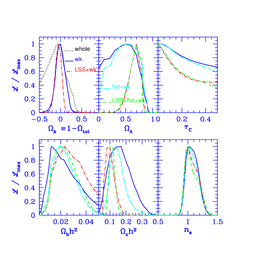
Figure 2.— 1D projected likelihood functions calculated for the CBIo140+DMR data. All panels include the weak-$h$ (solid dark blue) and LSS+weak-$h$(short-dash-dotted red) priors. (LSS is the large-scale structure prior.) The $\Omega_{k}$ panel also shows what the whole ${\cal C}_{\ell}$-database gives before the weak-$h$ prior is imposed (black dotted). We note that even in the absence of CMB data there is a bias towards the closed models (Lange et al., 2001). In the other panels, flat+weak-$h$ (long-dashed-dotted light blue) and LSS+flat+weak-$h$ (dashed green) are plotted. Notice how stable the $n_{s}$ determination is, independent of priors. We see here that, under priors ranging from the weak-$h$ prior to the weak-$h$+LSS+flat priors, the CBI provides a useful measure of four out of the six fundamental parameters shown. This is independent of the first acoustic peak, where the CBI has low sensitivity, and is also largely independent of the spectrum below $\ell\sim 610$ for all but $\Omega_{b}h^{2}$ (see text).

The primary results of the CBI cosmological parameter extraction are shown in Table 3 and Figure 2. These show parameter determinations after marginalization over all other parameters for the CBIo140+DMR dataset and for all combinations of the priors described in § 2.

Table 3Cosmic Parameters for Various Priors using CBIo140+DMR

Priors	$\Omega_{\rm tot}$	$n_{s}$	$\Omega_{b}h^{2}$	$\Omega_{\rm cdm}h^{2}$	$\Omega_{\Lambda}$	$\Omega_{m}$	$\Omega_{b}$	$h$	Age	$\tau_{c}$
wk-$h$	$1.00^{0.11}_{0.12}$	$1.08^{0.11}_{0.10}$	$0.023^{0.016}_{0.010}$	$0.16^{0.08}_{0.07}$	$0.43^{0.25}_{0.28}$	$0.59^{0.22}_{0.22}$	$0.083^{0.053}_{0.053}$	$0.58^{0.11}_{0.11}$	$13.9^{2.2}_{2.2}$	$<0.66$
wk-$h$+LSS	$1.05^{0.08}_{0.08}$	$1.07^{0.13}_{0.10}$	$0.029^{0.015}_{0.012}$	$0.10^{0.04}_{0.03}$	$0.67^{0.10}_{0.13}$	$0.39^{0.12}_{0.12}$	$0.095^{0.055}_{0.055}$	$0.60^{0.12}_{0.12}$	$15.4^{2.1}_{2.1}$	$<0.66$
wk-$h$+SN	$1.03^{0.08}_{0.08}$	$1.11^{0.11}_{0.11}$	$0.028^{0.016}_{0.012}$	$0.10^{0.05}_{0.04}$	$0.71^{0.08}_{0.09}$	$0.33^{0.08}_{0.08}$	$0.076^{0.046}_{0.046}$	$0.65^{0.12}_{0.12}$	$14.7^{2.4}_{2.4}$	$<0.67$
wk-$h$+LSS+SN	$1.04^{0.08}_{0.08}$	$1.11^{0.11}_{0.10}$	$0.029^{0.016}_{0.012}$	$0.10^{0.04}_{0.03}$	$0.72^{0.07}_{0.07}$	$0.32^{0.08}_{0.08}$	$0.082^{0.047}_{0.047}$	$0.64^{0.11}_{0.11}$	$15.0^{2.2}_{2.2}$	$<0.67$
flat+wk-$h$	(1.00)	$1.07^{0.11}_{0.10}$	$0.023^{0.010}_{0.008}$	$0.15^{0.06}_{0.04}$	$0.47^{0.25}_{0.27}$	$0.54^{0.24}_{0.24}$	$0.068^{0.028}_{0.028}$	$0.60^{0.12}_{0.12}$	$14.0^{1.4}_{1.4}$	$<0.65$
flat+wk-$h$+LSS	(1.00)	$1.05^{0.15}_{0.09}$	$0.024^{0.011}_{0.009}$	$0.11^{0.02}_{0.02}$	$0.67^{0.10}_{0.13}$	$0.34^{0.12}_{0.12}$	$0.057^{0.020}_{0.020}$	$0.66^{0.11}_{0.11}$	$14.2^{1.3}_{1.3}$	$<0.62$
flat+wk-$h$+SN	(1.00)	$1.10^{0.12}_{0.11}$	$0.025^{0.011}_{0.009}$	$0.11^{0.03}_{0.02}$	$0.70^{0.07}_{0.07}$	$0.30^{0.07}_{0.07}$	$0.052^{0.017}_{0.017}$	$0.70^{0.09}_{0.09}$	$13.8^{1.4}_{1.4}$	$<0.65$
flat+wk-$h$+LSS+SN	(1.00)	$1.08^{0.11}_{0.09}$	$0.025^{0.011}_{0.009}$	$0.11^{0.03}_{0.02}$	$0.71^{0.06}_{0.06}$	$0.29^{0.06}_{0.06}$	$0.053^{0.016}_{0.016}$	$0.69^{0.09}_{0.09}$	$13.9^{1.3}_{1.3}$	$<0.63$
flat+HST-$h$	(1.00)	$1.09^{0.12}_{0.10}$	$0.026^{0.010}_{0.009}$	$0.13^{0.07}_{0.04}$	$0.65^{0.12}_{0.20}$	$0.38^{0.18}_{0.18}$	$0.058^{0.022}_{0.022}$	$0.68^{0.08}_{0.08}$	$13.3^{1.3}_{1.3}$	$<0.65$
flat+HST-$h$+LSS	(1.00)	$1.09^{0.13}_{0.10}$	$0.026^{0.010}_{0.009}$	$0.11^{0.03}_{0.02}$	$0.71^{0.07}_{0.08}$	$0.29^{0.08}_{0.08}$	$0.054^{0.019}_{0.019}$	$0.70^{0.08}_{0.08}$	$13.8^{1.1}_{1.1}$	$<0.64$
flat+HST-$h$+SN	(1.00)	$1.10^{0.12}_{0.11}$	$0.026^{0.010}_{0.009}$	$0.12^{0.03}_{0.03}$	$0.71^{0.06}_{0.06}$	$0.29^{0.07}_{0.07}$	$0.052^{0.017}_{0.017}$	$0.71^{0.07}_{0.07}$	$13.6^{1.2}_{1.2}$	$<0.65$
flat+HST-$h$+LSS+SN	(1.00)	$1.08^{0.11}_{0.09}$	$0.026^{0.010}_{0.009}$	$0.11^{0.02}_{0.02}$	$0.71^{0.06}_{0.05}$	$0.29^{0.06}_{0.06}$	$0.054^{0.017}_{0.017}$	$0.70^{0.07}_{0.07}$	$13.7^{1.1}_{1.1}$	$<0.63$

Note. — Estimates of the 6 external cosmological parameters that characterize our fiducial minimal-inflation model set as progressively more restrictive prior probabilities are imposed. ($\tau_{C}$ is put at the end because it is relatively poorly constrained, even with the priors.) Central values and $1\sigma$ limits for the 6 parameters are found from the 16%, 50% and 84% integrals of the marginalized likelihood. For the other “derived” parameters listed, the values are means and variances of the variables calculated over the full probability distribution. wk-$h$ requires $0.45<h<0.90$, Age $>10$ Gyr, and $\Omega_{m}>0.1$. The sequence shows what happens when LSS, SN and LSS+SN priors are imposed. While the first four rows allow $\Omega_{\rm tot}$ to be free, the next four have $\Omega_{\rm tot}$ pegged to unity, a number strongly suggested by the CMB data. The final 4 rows show the “strong-$h$” prior, a Gaussian centered on $h=0.71$ with dispersion $\pm 0.076$, obtained for the Hubble key project. When the $1\sigma$ errors are large it is usual that there is a poor detection, and sometimes there can be multiple peaks in the 1D projected likelihood.

4.1.1 The Geometry and the Primordial Fluctuation Spectrum

We begin the cosmological parameters discussion by considering $\Omega_{\rm tot}$ and $n_{s}$. We see from Table 3 that under the weak-$h$ prior assumption the combination CBIo140+DMR yields $\Omega_{\rm tot}=1.00_{-0.12}^{+0.11}$ and $n_{s}=1.08_{-0.10}^{+0.11}$.

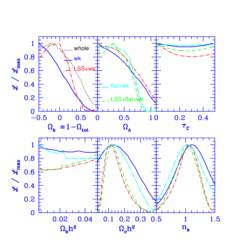
Figure 3.— Results obtained using DMR alone. This gives an idea of the role of the LSS prior in sharpening up detections for DMR. Note that DMR did reasonably well by itself in first indicating for this class of models that $n_{s}\sim 1$ (e.g., Bond, 1996). Of course it could not determine $\omega_{b}$ and the structure in $\Omega_{k}$ and $\Omega_{\Lambda}$ can be traced to ${\cal C}_{\ell}$-database constraints (Lange et al., 2001). Comparison with Fig. 2 shows the greatly improved constraints when the CBI data are added.

To illustrate clearly the constraints that the CBI observations impose we show in Figure 3 the likelihoods obtained from DMR alone under the various priors. Note that the $\Omega_{\rm k}$ likelihood curve is very broad. This figure shows that the above tight cosmological constraints do not arise from the priors. Rather, the other experiments nicely complement the CMB, greatly enhancing the discriminatory power of any single data set. These likelihood curves should also be contrasted with the “prior-only” likelihood curves presented by Lange et al. (2001). The results of adding the CBI data are shown in Figure 2. The effect of combining the CBI data with the DMR data under the LSS prior is to reduce the uncertainties in $\Omega_{\rm tot}$ — with these priors $\Omega_{\rm tot}=1.05_{-0.08}^{+0.08}$. Note that the uncertainties on $n_{s}$ are almost independent of the priors, and are always $\sim 10\%$.

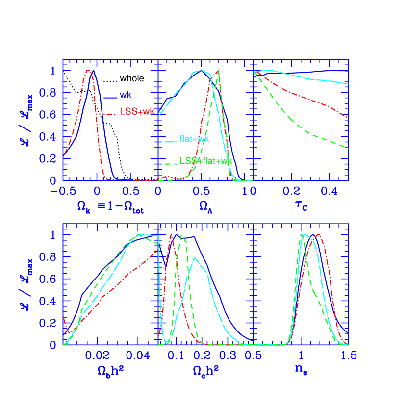
Figure 4.— Same as Fig. 2, except that CBI data at $\ell<610$ have been discarded. We see that, under the weak-$h$ and LSS+weak-$h$ priors, $\Omega_{\rm k}$ is peaked near zero, as is the case for the whole data set, showing that in the CBI data the evidence for a flat universe is coming from the $\ell$-range above the second acoustic peak where damping dominates, as well as from the lower-$\ell$ range. We see here that under increasingly restrictive priors the CBI data at $\ell>610$ provide useful constraints on $n_{s}$, $\Omega_{m}h^{2}$ and $\Omega_{\Lambda}$, showing that these results are driven by the shape (and level) of the spectrum at high-$\ell$ independent of the results at low-$\ell$. Note, however, that when the CBI data are restricted to $\ell>610$ they do not provide a useful measure of $\Omega_{b}h^{2}$ (compare with Fig. 2).

The CBI has very little sensitivity at $\ell<400$, thus these determinations of $\Omega_{\rm tot}$ and $n_{s}$ are basically independent of the first acoustic peak. We have explored the degree to which the CBI results depend on the low-$\ell$ data by eliminating the band-powers at $\ell<610$, and running the same sequence of tests of increasingly restrictive priors. The results for the cut at $\ell=610$ are shown in Figure 4 and in Table 4. The likelihood is still sharply peaked at $\Omega_{\rm tot}\sim 1$ even though the data from the region of the first and second peaks has been discarded.

The effect of discarding the data at $\ell<610$ on $n_{s}$ is seen in Figure 4. We see that the likelihood again peaks near unity, showing that the determination of a near scale-invariant fluctuation spectrum is not dependent on the first or second acoustic peaks in the CBI data.

We conclude that both the geometry and the fluctuation spectrum are highly consistent with the predictions of the minimal inflationary theory, and that this consistency applies even when the data at $\ell<610$, corresponding to the regions of the first and second acoustic peaks, are discarded. These results on $\Omega_{\rm tot}$ and $n_{s}$ are therefore independent of previous results based on observations over the multipole range of the first and second acoustic peaks. The $\ell<610$ and $\ell>610$ regions of the angular spectrum indicate a consistent power law for the primordial spectrum, for the minimal models we consider, over the range of scales covered by the observations which now extend down to the scales of clusters of galaxies probed directly by LSS studies.

4.1.2 The Non-Baryonic and Baryonic Matter Densities and the Cosmological Constant

The constraints on the density in dark matter, $\omega_{\rm cdm}$, and the cosmological constant, $\Omega_{\Lambda}$ are shown in Figure 2. One sees that these are tightly constrained when the LSS prior is added. The effect of adding the CBI data can be seen by comparing the weak-$h$+LSS prior results in Figure 3 with those in Figure 2. We see that the CBI data reduce the uncertainties dramatically, and that $\omega_{\rm cdm}=0.10_{-0.03}^{+0.04}$ and $\Omega_{\Lambda}=0.67_{-0.13}^{+0.10}$ for the weak-$h$+LSS priors case. If, in addition, we assume a flat geometry, the uncertainties in the dark matter density are further improved, $\omega_{\rm cdm}=0.11_{-0.02}^{+0.02}$, while those for the cosmological constant are the same. We see from Figure 4 and from Table 4 that the constraints on the dark matter density are also reasonably tight when the data at $\ell<610$ are discarded. The results on $\Omega_{\Lambda}$ are little changed when the data below $\ell=610$ are discarded although the uncertainties are larger, as can be seen by comparing Figure 4 with Figure 2. Thus these results on $\omega_{\rm cdm}$ and $\Omega_{\Lambda}$ are also established over the high-$\ell$ range independent of the first and second acoustic peaks.

The fractional CBI constraints on the baryonic matter density are not nearly as tight as those on non-baryonic matter. With the weak-$h$+LSS+flat priors, we see from Table 3 that $\omega_{b}=0.024_{-0.009}^{+0.011}$. This is consistent with the results from Big Bang nucleosynthesis (Olive et al., 1999; Burles et al., 2000; Tytler et al., 2000). When we discard the data below $\ell=610$, we do not yet have a useful constraint on $\Omega_{b}h^{2}$ (see Figure 4). Although weaker, the potential constraints on the baryonic matter density from the high-$\ell$ region of the spectrum are important because this is, in principle, a direct and independent way of measuring $\Omega_{b}h^{2}$.

From the combination of the densities in both baryonic and non-baryonic matter, we see that the CBI provides compelling evidence for a matter density significantly lower than the critical density required to close the universe, with $\Omega_{m}=0.34\pm 0.12$, with $\Omega_{b}=0.057\pm 0.020$ in baryons. This result, combined with the flat geometry, requires a significant energy component of the universe to be supplied by something other than matter, and this we assume under our minimal inflationary scenario to be the cosmological constant.

4.1.3 The Hubble Constant and the Age of the Universe

Significant measures of the Hubble constant and the age of the universe are again obtained under the weak-$h$+LSS+flat priors (see Table 3). We find, under these priors, that $h=0.66\pm 0.11$ and $t_{0}=14.2\pm 1.3$ Gyr. These are in excellent agreement with recent determinations of the Hubble constant (Mould et al., 2000; Freedman et al., 2001) and the ages of the oldest stars in globular clusters.

4.2. Further Robustness Tests

We have carried out a large number of tests, further to those described in the previous section, of the parameter extraction from the CBI observations. We describe some of the more important of these tests in this section.

Table 4CBI Tests and Comparisons

Priors	$\Omega_{\rm tot}$	$n_{s}$	$\Omega_{b}h^{2}$	$\Omega_{\rm cdm}h^{2}$	$\Omega_{\Lambda}$	$\Omega_{m}$	$\Omega_{b}$	$h$	Age	$\tau_{c}$
CBIo140
wk-$h$	$1.00^{0.11}_{0.12}$	$1.08^{0.11}_{0.10}$	$0.023^{0.016}_{0.010}$	$0.16^{0.08}_{0.07}$	$0.43^{0.25}_{0.28}$	$0.59^{0.22}_{0.22}$	$0.083^{0.053}_{0.053}$	$0.58^{0.11}_{0.11}$	$13.9^{2.2}_{2.2}$	$<0.66$
flat+wk-$h$	(1.00)	$1.07^{0.11}_{0.10}$	$0.023^{0.010}_{0.008}$	$0.15^{0.06}_{0.04}$	$0.47^{0.25}_{0.27}$	$0.54^{0.24}_{0.24}$	$0.068^{0.028}_{0.028}$	$0.60^{0.12}_{0.12}$	$14.0^{1.4}_{1.4}$	$<0.65$
flat+wk-$h$+LSS	(1.00)	$1.05^{0.15}_{0.09}$	$0.024^{0.011}_{0.009}$	$0.11^{0.02}_{0.02}$	$0.67^{0.10}_{0.13}$	$0.34^{0.12}_{0.12}$	$0.057^{0.020}_{0.020}$	$0.66^{0.11}_{0.11}$	$14.2^{1.3}_{1.3}$	$<0.62$
CBIe140
wk-$h$	$0.96^{0.14}_{0.13}$	$1.10^{0.11}_{0.11}$	$0.016^{0.013}_{0.007}$	$0.18^{0.08}_{0.07}$	$0.37^{0.28}_{0.26}$	$0.62^{0.23}_{0.23}$	$0.059^{0.044}_{0.044}$	$0.60^{0.11}_{0.11}$	$13.3^{2.1}_{2.1}$	$<0.66$
flat+wk-$h$	(1.00)	$1.08^{0.11}_{0.10}$	$0.018^{0.009}_{0.006}$	$0.15^{0.05}_{0.04}$	$0.44^{0.26}_{0.27}$	$0.56^{0.24}_{0.24}$	$0.059^{0.025}_{0.025}$	$0.58^{0.11}_{0.11}$	$14.1^{1.3}_{1.3}$	$<0.66$
flat+wk-$h$+LSS	(1.00)	$1.06^{0.14}_{0.10}$	$0.020^{0.010}_{0.007}$	$0.11^{0.02}_{0.02}$	$0.68^{0.09}_{0.13}$	$0.32^{0.11}_{0.11}$	$0.049^{0.019}_{0.019}$	$0.67^{0.11}_{0.11}$	$14.3^{1.3}_{1.3}$	$<0.63$
CBIo140$(\ell>610)$
wk-$h$	$1.06^{0.15}_{0.14}$	$1.14^{0.15}_{0.13}$	$0.068^{0.065}_{0.036}$	$0.15^{0.10}_{0.08}$	$0.44^{0.26}_{0.28}$	$0.71^{0.26}_{0.26}$	$0.264^{0.207}_{0.207}$	$0.59^{0.11}_{0.11}$	$13.1^{1.8}_{1.8}$	$<0.67$
flat+wk-$h$	(1.00)	$1.10^{0.12}_{0.10}$	$0.047^{0.056}_{0.019}$	$0.18^{0.07}_{0.07}$	$0.41^{0.22}_{0.26}$	$0.62^{0.23}_{0.23}$	$0.188^{0.166}_{0.166}$	$0.63^{0.11}_{0.11}$	$12.6^{1.4}_{1.4}$	$<0.66$
flat+wk-$h$+LSS	(1.00)	$1.05^{0.14}_{0.09}$	$0.041^{0.017}_{0.017}$	$0.13^{0.03}_{0.03}$	$0.66^{0.09}_{0.13}$	$0.35^{0.11}_{0.11}$	$0.082^{0.037}_{0.037}$	$0.71^{0.11}_{0.11}$	$13.1^{1.4}_{1.4}$	$<0.62$
CBIo200
wk-$h$	$1.12^{0.13}_{0.14}$	$1.14^{0.12}_{0.11}$	$0.048^{0.023}_{0.024}$	$0.22^{0.09}_{0.08}$	$0.36^{0.27}_{0.25}$	$0.82^{0.32}_{0.32}$	$0.152^{0.088}_{0.088}$	$0.58^{0.10}_{0.10}$	$12.8^{1.9}_{1.9}$	$<0.67$
flat+wk-$h$	(1.00)	$1.07^{0.11}_{0.09}$	$0.025^{0.015}_{0.010}$	$0.19^{0.09}_{0.07}$	$0.41^{0.25}_{0.26}$	$0.61^{0.24}_{0.24}$	$0.071^{0.033}_{0.033}$	$0.63^{0.11}_{0.11}$	$12.6^{1.7}_{1.7}$	$<0.64$
flat+wk-$h$+LSS	(1.00)	$1.04^{0.14}_{0.08}$	$0.028^{0.014}_{0.011}$	$0.12^{0.03}_{0.02}$	$0.68^{0.09}_{0.13}$	$0.33^{0.11}_{0.11}$	$0.061^{0.025}_{0.025}$	$0.70^{0.11}_{0.11}$	$13.6^{1.4}_{1.4}$	$<0.59$
CBIdeep
wk-$h$	$1.09^{0.11}_{0.24}$	$1.16^{0.15}_{0.14}$	$0.078^{0.070}_{0.049}$	$0.21^{0.11}_{0.12}$	$0.42^{0.31}_{0.29}$	$0.85^{0.32}_{0.32}$	$0.261^{0.190}_{0.190}$	$0.61^{0.10}_{0.10}$	$12.2^{1.8}_{1.8}$	$<0.67$
flat+wk-$h$	(1.00)	$1.05^{0.12}_{0.11}$	$0.050^{0.072}_{0.034}$	$0.20^{0.09}_{0.14}$	$0.37^{0.26}_{0.25}$	$0.65^{0.24}_{0.24}$	$0.189^{0.188}_{0.188}$	$0.64^{0.11}_{0.11}$	$12.2^{1.9}_{1.9}$	$<0.66$
flat+wk-$h$+LSS	(1.00)	$1.03^{0.13}_{0.11}$	$0.055^{0.064}_{0.035}$	$0.13^{0.04}_{0.04}$	$0.55^{0.16}_{0.28}$	$0.50^{0.23}_{0.23}$	$0.187^{0.179}_{0.179}$	$0.66^{0.13}_{0.13}$	$12.9^{2.0}_{2.0}$	$<0.65$
DASI+CBIo140
wk-$h$	$1.05^{0.05}_{0.06}$	$1.01^{0.11}_{0.07}$	$0.023^{0.004}_{0.004}$	$0.12^{0.04}_{0.04}$	$0.55^{0.17}_{0.22}$	$0.51^{0.19}_{0.19}$	$0.077^{0.024}_{0.024}$	$0.56^{0.10}_{0.10}$	$15.2^{1.5}_{1.5}$	$<0.63$
flat+wk-$h$	(1.00)	$0.99^{0.08}_{0.05}$	$0.021^{0.004}_{0.003}$	$0.14^{0.03}_{0.03}$	$0.56^{0.18}_{0.26}$	$0.46^{0.21}_{0.21}$	$0.057^{0.017}_{0.017}$	$0.62^{0.11}_{0.11}$	$13.9^{0.8}_{0.8}$	$<0.39$
flat+wk-$h$+LSS	(1.00)	$1.00^{0.10}_{0.06}$	$0.022^{0.004}_{0.004}$	$0.12^{0.02}_{0.02}$	$0.66^{0.09}_{0.10}$	$0.33^{0.10}_{0.10}$	$0.048^{0.009}_{0.009}$	$0.68^{0.09}_{0.09}$	$13.8^{0.8}_{0.8}$	$<0.42$
DASI+Boom+CBIo140
wk-$h$	$1.03^{0.05}_{0.05}$	$0.95^{0.09}_{0.05}$	$0.022^{0.003}_{0.003}$	$0.13^{0.03}_{0.03}$	$0.52^{0.18}_{0.20}$	$0.52^{0.19}_{0.19}$	$0.074^{0.022}_{0.022}$	$0.56^{0.10}_{0.10}$	$15.0^{1.4}_{1.4}$	$<0.52$
flat+wk-$h$	(1.00)	$0.94^{0.06}_{0.04}$	$0.021^{0.002}_{0.002}$	$0.14^{0.03}_{0.03}$	$0.55^{0.18}_{0.28}$	$0.48^{0.21}_{0.21}$	$0.058^{0.016}_{0.016}$	$0.61^{0.11}_{0.11}$	$14.0^{0.5}_{0.5}$	$<0.31$
flat+wk-$h$+LSS	(1.00)	$0.94^{0.08}_{0.04}$	$0.022^{0.002}_{0.002}$	$0.13^{0.02}_{0.02}$	$0.63^{0.09}_{0.11}$	$0.37^{0.10}_{0.10}$	$0.051^{0.008}_{0.008}$	$0.65^{0.07}_{0.07}$	$13.9^{0.5}_{0.5}$	$<0.36$
all-data
wk-$h$	$1.04^{0.05}_{0.05}$	$0.98^{0.10}_{0.06}$	$0.023^{0.003}_{0.003}$	$0.12^{0.03}_{0.03}$	$0.55^{0.17}_{0.20}$	$0.49^{0.18}_{0.18}$	$0.075^{0.023}_{0.023}$	$0.56^{0.11}_{0.11}$	$15.1^{1.4}_{1.4}$	$<0.57$
flat+wk-$h$	(1.00)	$0.96^{0.09}_{0.05}$	$0.022^{0.003}_{0.002}$	$0.13^{0.03}_{0.03}$	$0.60^{0.15}_{0.26}$	$0.42^{0.20}_{0.20}$	$0.055^{0.015}_{0.015}$	$0.64^{0.11}_{0.11}$	$13.9^{0.5}_{0.5}$	$<0.35$
flat+wk-$h$+LSS	(1.00)	$0.97^{0.09}_{0.05}$	$0.022^{0.003}_{0.002}$	$0.12^{0.02}_{0.02}$	$0.66^{0.09}_{0.12}$	$0.35^{0.10}_{0.10}$	$0.051^{0.008}_{0.008}$	$0.66^{0.08}_{0.08}$	$13.8^{0.5}_{0.5}$	$<0.39$

Note. — Cosmological parameter estimates as in Table 3, except for a variety of data combinations which test and compare results. Only the wk-$h$, flat+wk-$h$ and flat+wk-h+LSS priors are shown.

The effects of discarding the CBI data at $\ell<610$ on the full suite of parameters and priors can be seen by comparing Table 3 and Table 4. In this cut, we discarded the first three bins of CBI data. It can be seen here that the constraints on cosmological parameters degrade gracefully as data are discarded. We have also tested the effect of discarding the first four bins of CBI data (i.e., up to $\ell=750$) and we find that the uncertainties continue to increase, as expected, but no large variations in the central values of the parameters are seen. It is clear, therefore, that the CBI results are robust in this regard.

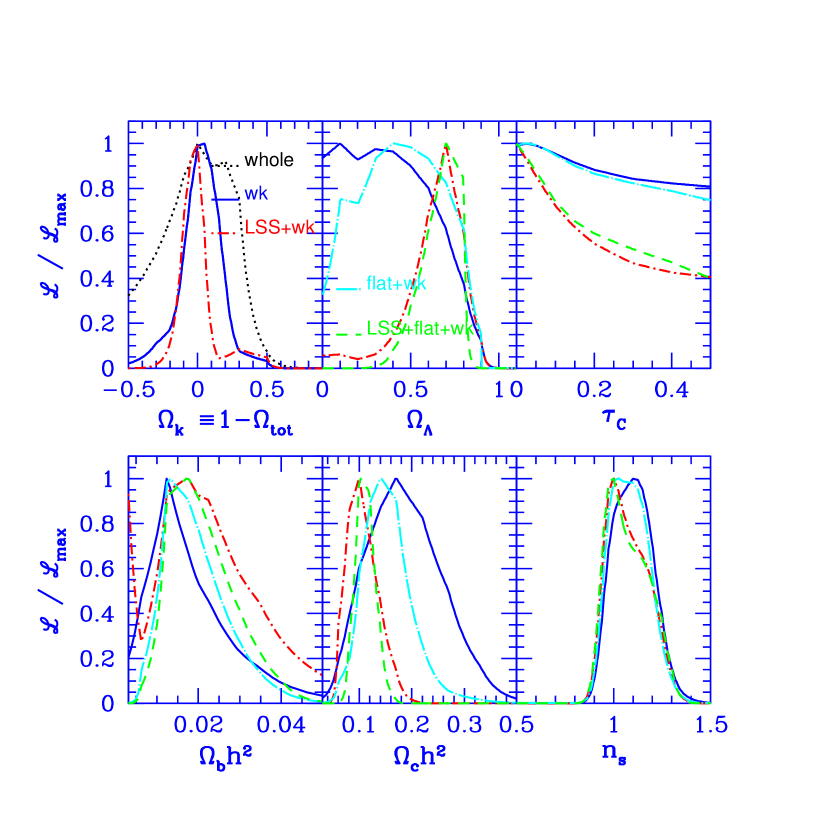
Figure 5.— Same as Fig. 2, except for CBIe140+DMR. By comparing this figure with Fig. 2, we see that the particular choice of bin boundaries does not make a significant difference to the parameter estimation. This can also be seen from the comparison of the even and odd binning cases in Table 4.

We have compared the results derived from the two alternate binnings of the data — the “odd” binning and the “even” binning. The results are shown in Figure 5, Figure 7, and Table 4. We see that the derived values of the parameters agree to within the uncertainties in all cases, and that the uncertainties are comparable. This comparison demonstrates clearly that there is no dependence of the cosmological results on the binning choice.

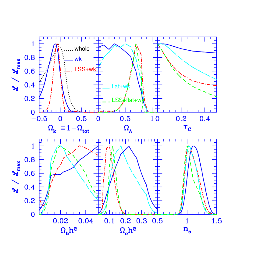
Figure 6.— Same as Fig. 2, except for the bin size, which is 200 here. By comparing this figure with Fig. 2, we see that the bin size does not make a large difference to the parameter estimation, excepting $\Omega_{b}h^{2}$, for which the $\Delta\ell=200$ binwidth case does not give a useful measurement. This can also be seen from the comparison of the $\Delta\ell=140$ and $\Delta\ell=200$ cases in Table 4.

We have also compared the values of the parameters extracted using bin widths of $\Delta\ell=140$ (Figure 2) and $\Delta\ell=200$ (Figure 6; see also Table 3 and Table 4). Comparison of these figures and the actual values and associated uncertainties shows that the cosmological results are in excellent agreement. The results are not strongly dependent on the bin width, although there is, of course, some loss of information at the larger bin width, which is reflected in the larger uncertainties.

We have also tested the effect of varying the residual source contribution on parameters. As expected from its small relative contribution, we find very little difference if we either assume our standard power value described in Papers II and III, allow for a 50% error in that estimate, or multiply the standard power by a factor of 2.25.

We end our discussion of tests of the cosmological parameter extraction from the CBI observations by showing projections of the full seven-dimensional likelihood function onto 2D contour plots of the likelihoods of various combinations of cosmological parameters $\{\omega_{\rm cdm},\Omega_{k},\omega_{b},\Omega_{\Lambda},n_{s}\}$ to illustrate further the consistency of the various CBI data subsets used throughout this work. These 2D contour plots provide a different insight into the tests of data consistency than do the 1D plots of the previous subsections, which can be illuminating. For example, they can show directly whether there are isolated multiple peaks in the likelihood surface, whereas this information is lost in the marginalization of the 1D plots.

In Paper III we showed the power spectra for the individual mosaic fields, and we found that the differences are not statistically significant. Here we derive constraints on the cosmological parameters from three sets of pairwise-combined mosaic fields. These give stronger constraints on parameters than the single fields and thus provide a stronger consistency check. We find there is good consistency between the three pairs, showing that no field is seriously discrepant with the other two, in agreement with our finding in Paper III that there are no significant differences between the spectra from the three fields. The agreement between the three pairs of fields can be seen in Figure 7, the results of the pairwise splitting of the three mosaic data sets. Displayed here are the 1- and 2-$\sigma$ contours for the odd binning of the $\Delta\ell=140$ data.

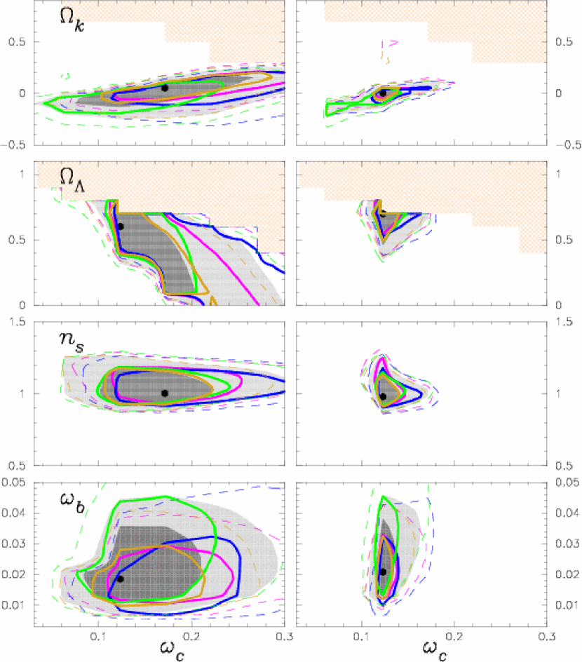
Figure 7.— Comparison of likelihood contours for the three pairwise combinations of the three mosaic fields for the CBIo140+ DMRdata. Full lines are $1\sigma$ and dashed lines are $2\sigma$ contours. The hatched regions indicate portions excluded by the range of parameters considered (see Table 1). The weak-$h$ prior applies in the $\omega_{\rm cdm}$–$\Omega_{k}$ panel and flat+weak-$h$ prior applies in the other panels. The plots on the left do not have the LSS prior, while those on the right do. The pairs of mosaics are as follows: 02h+20h (magenta); 02h+14h (dark blue); 14h+20h (green). The results for the three fields combined are shown by the dark grey regions ($1\sigma$) and the light grey regions ($2\sigma$). For comparison, the results for the alternate binning (CBIe140+ DMR) are shown by the gold contours. Comparison of the plots on the left with those on the right show the dramatic impact of the LSS prior on the $\omega_{\rm cdm}$ determination, its role in $\Omega_{\Lambda}$ determination, and its relatively small impact in the other variable directions. The dramatic reduction in the uncertainties in $\omega_{\rm cdm}$ is due to the combined effects of the CBI data and the LSS prior (see text). (For this comparison, the slightly smaller database in (Lange et al., 2001) was used rather than that in Table 1.)

The effect of introducing the LSS prior is also shown in Figure 7. It primarily reduces the uncertainties in $\omega_{\rm cdm}$. Note that it is the combination of the CBI observations and the LSS prior that accomplishes this. This can be seen by comparing Figure 3, in which the uncertainties under the LSS prior are large, to Figure 2 in which the CBI data have been included and the uncertainties are greatly reduced.

A 2D comparison of the parameters extracted under the two binning schemes is shown in Figure 7, with the effect of adding the LSS prior also shown. These should be compared with Figure 2 and Figure 5, and with the values given in Table 4. We see here, once again, that the consistency between these two binning schemes is excellent.

One of the caveats that is important to bear in mind when dealing with 7D-plus parameter spaces is that the limits derived from projection onto one or two directions in parameter space by full Bayesian marginalization (integration) over the other variables can be misleading in certain cases. For example, highly likely models which exist far from broad likelihood peaks may be ruled out. With all of the CMB data, many of the variables are well localized and this is not a big problem. However, near degeneracies among cosmological parameters do exist in these inflation model spaces (Efstathiou & Bond, 1999). The correlations can be quantified by considering parameter eigenmodes (e.g., Bond, 1996; Bond, Efstathiou & Tegmark, 1997; Efstathiou & Bond, 1999; Lange et al., 2001) which yield linear combinations of the ${\cal C}_{\ell}$-database variables that give orthogonal errors in the neighborhood of the maximum likelihood values.

For CBIo140+DMR with weak-$h$ prior, two combinations are determined to better than 10% and two others to 15%. The three best-determined values involve a predominantly $n_{s}$ combination, with $\tau_{C}$ and amplitude mixed in, and then, somewhat remarkably, a predominantly $\Omega_{k}$ combination, followed by a mix of many parameters, including amplitude, $\Omega_{\Lambda}$ and $\omega_{cdm}$. With all-data, weak-$h$ gives 4 combinations to better than 10%. The first two are different mixes of $n_{s}$ and $\Omega_{k}$, next is mainly $\omega_{b}$ and then a $\omega_{\rm cdm}$–$\omega_{b}$–$\Omega_{\Lambda}$ combination. LSS sharpens up the fourth eigenmode especially.

In conclusion we would emphasize the excellent overall consistency of the cosmological parameters extracted from the CBI mosaic and deep observations. It was shown in Papers II and III that various subsets of the data are consistent with each other to within the levels expected, given the uncertainties. Here we have shown that the cosmological parameters derived from different subsets of the data, and from different binning schemes and bin widths, are also self-consistent. We conclude that both the CBI data themselves and the cosmological parameter extraction from the CBI observations are robust.

5. Optimal Power Spectra

In this section, we apply the parameter-estimation methods of Appendix 3 to combine power spectra derived with different bandpowers and with different window functions onto a common set of bands. A byproduct is the determination of how consistent the power spectra are and the values of various experimental parameters that can be adjusted to increase agreement (e.g., adjustments to the flux density scale). For all of the bandpower applications, a best-fit model was used for ${\cal C}_{\ell}^{(s)}$ rather than flat bandpowers.

5.1. CBI Optimal Power Spectra

In addition to the extraction of the optimal power spectrum for the whole CBI data set, we are interested in extracting optimal power spectra for subsets of the data. Although these optimal spectra are not used in the estimation of the cosmological parameters, they do provide an invaluable means of comparing the various data sets, and, of course, of comparing the CBI data to other CMB data sets.

We begin the extraction of optimal spectra by examining the pairwise combinations of the three mosaic fields. Thus we combine pairs of the three mosaic fields (02^h, 14^h, and 20^h). These are separated by about 6^h in RA, which is sufficient to treat them as independent fields and uncorrelated data sets. When combining the fields we do not include separate calibration errors since these are common to all fields, and we assume no error on the estimate of the residual source component. The NVSS sources are projected out as described in Papers II and III, and that is included in this treatment.

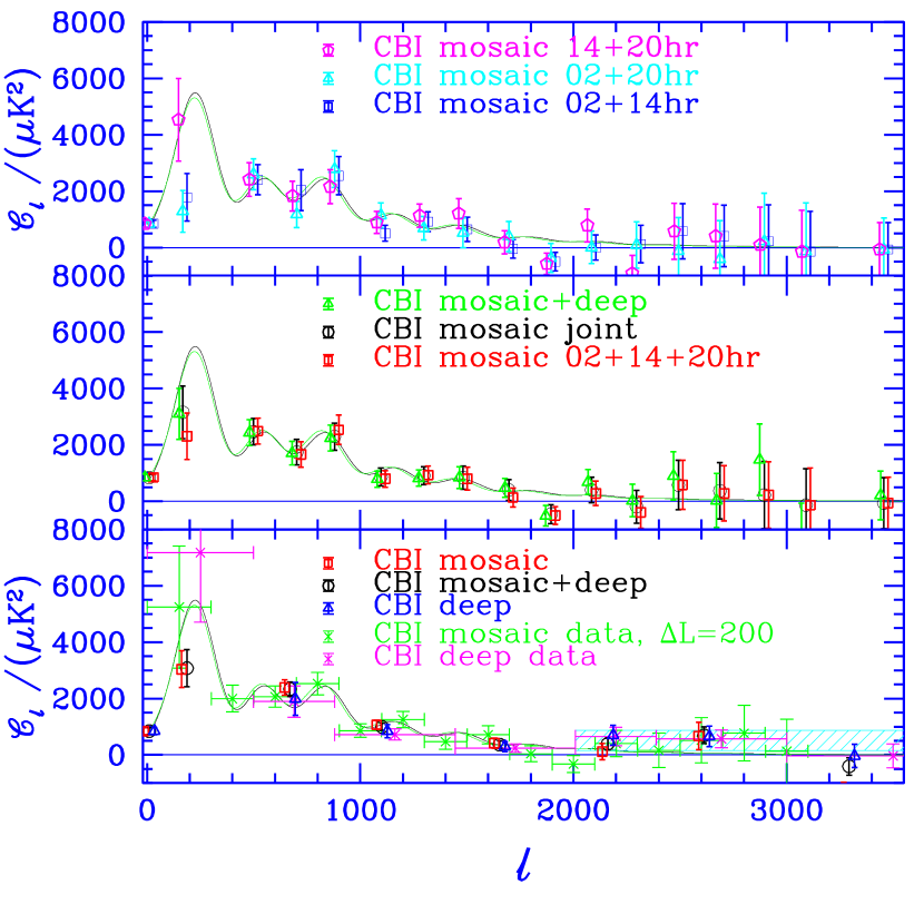
Figure 8.— Optimal power spectra from CBI observations. Upper panel: Consistency between pairs of CBIo140 fields. Here the CBIo140 data have been re-binned to the CBIo200 bands for the purpose of comparison with other data sets (see text). At low-$\ell$ the errors are dominated by sample variance, which is a fraction of the fitted band-power — thus the apparent discrepancy between the pairs in the lowest-$\ell$ bin, due to the 02h field, is not significant (see Paper III). The best fit model, under the weak-$h$ and flat+weak-$h$ priors, to the DMR+CBIo140 data (black curve) has $\{\Omega_{\rm{tot}}$, $\Omega_{\Lambda}$, $\Omega_{b}h^{2}$, $\Omega_{\rm cdm}h^{2}$, $n_{s}$, $\tau_{C}\}$=$\{1.0,0.6,0.0225,0.12,0.95,0.025\}$. The best fit model, under the weak-$h$, flat+weak-$h$ and flat+weak-$h$+LSS priors, for ALL-data (magenta curve) has parameters $\{1.0,0.5,0.02,0.14,0.925,0\}$. Middle panel: Combined joint 3-field CBIo140 and CBIdeep power spectra denoted by the green triangles; black circles denote the joint 3-field CBIo140 spectrum and red squares denote the 3 CBIo140 fields when combined as with the pair cases. The results are stable independent of whether even or odd binning is used. Lower panel: The CBIo200 and CBIdeep data are shown together with optimal spectra for deep, mosaic and deep+mosaic on the standard CBIdeep bands.

The upper panel of Figure 8 compares the combined spectra for the three pairs of mosaic fields. The center panel shows the combination of the three individual field spectra, the spectrum obtained from the joint analysis of the three fields (Paper III), and the combination of all six mosaic and deep fields. We have separated the upper and center panels for clarity, but when plotted together they show excellent consistency between all the combinations we have considered. In the spectra shown here, the CBIo140 data have been used and combined onto the $\Delta\ell$=200 bins. We find excellent agreement between the extracted optimal spectra, regardless of whether the CBIe140 or CBIo200 data are used. This shows not only that the extracted data are self-consistent, but also that the band-to-band correlations are being treated correctly. We see from the upper panel of Figure 8 that the agreement of the pairs is robust. This result is related to that obtained by comparing the power spectra for each individual mosaic field shown in Paper III. These show excursions among the power spectra for individual fields, although, as shown in Paper III, these excursions are not statistically significant. The pair-combined spectra shown here, with their increased statistical weights, indicate again that the excursions are compatible with expectations.

The three deep fields are single pointings with long integration times. Since the deep observations have better signal-to-noise ratios in the $\ell>2000$ range, it is useful to combine the deep spectra with the mosaic spectra, which have less cosmic variance at low $\ell$. One point to note is that two of the deep fields are embedded in the mosaic fields. However, the data used for the mosaics are only a subset of the data used in the the deep fields analysis, corresponding to the typical integration time on an individual mosaic pointing, which is about four hours. We therefore expect the correlations between the deep and mosaic data to be small and we ignore them when forming the optimal spectra. The center panel of Figure 8 compares the combined CBIdeep and joint CBIo140 data with those from just the joint CBIo140. Both cases use top hat window functions and are mapped onto the $\Delta\ell=200$ mosaic binning. The excess power anomaly seen in the deep data is not that evident with these relatively narrow bands, and the basic result is good agreement between the two.

The lower panel of Figure 8 compares the mosaic, deep, and mosaic+deep optimal power using the much coarser CBIdeep $\Delta\ell$ binning. This is similar to Figure 14 of Paper III, for which the mosaic data were evaluated directly in the CBI-pipeline analysis onto the CBIdeep bands. Here we have obtained a similar result by using only the CBIo140 data: although there is no detection of mosaic power at $\ell\sim 2200$, there is agreement in enhanced power levels at $\ell\sim 2700$, although the larger $1\sigma$ mosaic confidence region is consistent with a “non-detection”. The joint deep+mosaic bandpower has slightly smaller errors than the deep-only case.

The combined spectrum shows a clear detection of the expected damping of the power out to $\ell\sim 2000$. Thus the unique experimental setup of the CBI has further validated the cosmological paradigm outlined in § 1 by confirming one of the key ingredients. Note the agreement in the excess power in the $\ell\sim 2700$ band (though errors differ). Further study is needed to confirm this excess, and, if confirmed, to determine the source of the power (see Paper VI for further discussion).

5.2. The Overall Optimal Spectrum

In this section we compare the ${\cal C}_{b}$ (band-power) spectrum from the CBI with the spectra obtained from some other CMB experiments, and we then combine the CBI data with the data from the BOOMERANG, DASI, MAXIMA, and VSA experiments in order to obtain a new optimal ${\cal C}_{b}$ spectrum out to $\ell=3500$. This represents a considerable extension of the optimal spectrum beyond the previous limit at $\ell\sim 1000$.

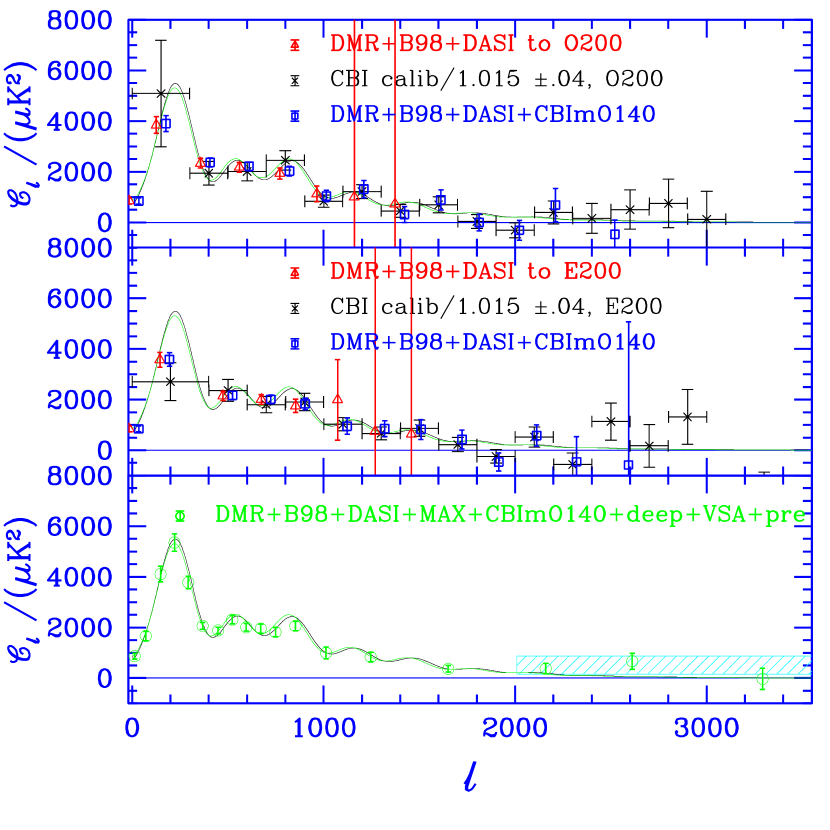
Figure 9.— Optimal power spectra: CBI compared to BOOMERANG and DASI. Upper panel: Joint CBIo200 power spectrum compared with optimal power spectra using BOOMERANG+DASI data (red triangles) and CBIo140+BOOMERANG+DASI data (dark blue circles) in the CBIo200 binning. The optimal spectra correspond to a maximum-likelihood fit to the power in bands for the three spectra, marginalized over beam and calibration uncertainty. The best fit curves shown are the same as in Fig. 8. Middle panel: same as the upper panel, but using the CBIe200 binning. Lower panel: The optimal spectrum for “all-data”, with a finer $\Delta\ell=75$ binning up to $\sim 800$, and deep binning at large $\ell$. The $\ell>2000$ excess found with the CBIdeep data is denoted by the light blue hatched region (95% confidence limit).

A comparison of the pre-CBI optimal spectrum with the optimal spectrum including the CBI deep and mosaic data is shown in Figure 9. As noted above, each experiment has unique binnings, band-to-band correlations, and calibration and beam errors. This makes a straightforward visual comparison difficult. To facilitate such comparisons, we therefore construct the optimal power spectrum for these experiments binned onto the $\Delta\ell=200$ CBI bins. Sample results are shown in Figure 9, along with some best-fit models. We see here that the agreement between the different CMB experiments is excellent. In the derivation of the optimal spectra shown here calibration uncertainties of 10% for BOOMERANG, 4% for DASI, 3.5% for VSA, and 4% for MAXIMA were included, together with beam uncertainties of 14% for BOOMERANG  and 5% for MAXIMA. For this purpose we need to include the calibration uncertainty for CBI, which we take to be a conservative 5%. These are all incorporated in the spectra, which leads to significant correlations among bands associated with the beam uncertainty. That is, one must be careful in using optimal spectra directly for parameter estimation since, although we can compute the Fisher matrix, we do not know the likelihood surface in detail.

We find the optimal power spectrum for BOOMERANG, DASI, and CBI requires a decrease in the temperature calibration by a factor $1.015\pm 0.04$ for CBI and $1.05\pm 0.05$ for BOOMERANG, and an increase by a factor $1.01\pm 0.04$ for DASI. The data also favor an increase in the BOOMERANG beam by $1.07\pm 0.04$ for the odd binning and $1.05\pm 0.04$ for the even binning. These values are consistent with the quoted errors in all cases. Indeed, assuming that the power spectra are derived from a single underlying spectrum, which the different experiments are sampling in their respective regions of the sky, one could use this technique to determine the calibrations and beams. For example, we note that the determinations for BOOMERANG have errors significantly smaller than the quoted uncertainties once they have been compared with the two sets of interferometer data, which have no beam uncertainties and much smaller calibration uncertainties.

An important caveat to these optimally-combined ${\cal C}_{b}$’s is that power spectra for the individual experiments were assumed to be independent. We have already commented on this for CBI deep and mosaic combinations. In addition DASI’s fields overlap about 5% of the BOOMERANG area, so there is correlation between BOOMERANG and DASI which is not taken into account in this treatment. The correlation would have to be addressed in order to claim absolute accuracy in the adjustment of experimental parameters.

Figure 9 shows very good agreement in the $300\lesssim\ell\lesssim 1000$ overlap region for BOOMERANG and DASI combined onto CBI points, and with all 3 experiments combined. (Note that the window functions for the combined spectra are top hats and not the $W_{B\ell}$ of the data points shown.) We also find the combined spectrum looks quite similar when all-data are used.

The method we used for Figure 9 has also been applied to construct optimal bandpowers for all of the above data (including CBIo140 and CBIdeep) with finer binning for $\ell<1000$. This variable binning makes use of the high quality BOOMERANG data with its intrinsic $\Delta\ell=50$ spacing at low $\ell$ and it also makes use of the high-$\ell$ coverage of the CBI (out to $\ell=3500$). The spectrum is compared in Paper VI with power spectra computed for the Sunyaev-Zeldovich effect, and will not be discussed further here.

6. Cosmological Parameter Estimates from Combined CMB Data

We test the consistency of our parameter estimations by comparing with different combinations of CBI and other data sets. We also derive estimates for the parameters from the full compilation of data available.

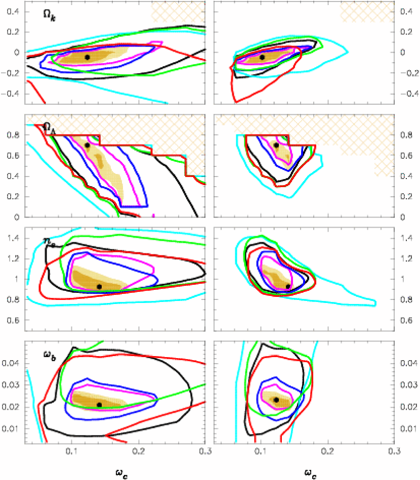
Figure 10.— Comparison of different experiments. 2-$\sigma$ likelihood contours for the weak-$h$ prior ($\omega_{\rm cdm}$–$\Omega_{k}$ panel) and flat+weak-$h$ prior for the rest, for the following CMB experiments in combination with DMR: CBIe140 (black), BOOMERANG (magenta), DASI (dark blue), MAXIMA (green), VSA (red) and “prior-CMB” = BOOMERANG-NA+TOCO+Apr99 data (light blue). Light brown region shows the 2-$\sigma$ contour when all of the data are taken together, dark brown shows the 1-$\sigma$ contour. The LSS prior has not been used in deriving the plots on the left, but it has for those on the right. The hatched regions indicate portions excluded by the range of parameters considered (see Table 1). This figure shows great consistency as well as providing a current snapshot of the collective CMB data results. Even without the LSS prior (or the HST-$h$ or SN1a priors), localization of the dark matter density is already occurring, but $\Omega_{\Lambda}$ still has multiple solutions. The inclusion of the SN1a and/or the HST-$h$ priors does not concentrate the bull’s-eye determinations much more for the all-data shaded case. Note that the expectation of minimal inflation models is that $\Omega_{k}\approx 0$, $n_{s}\approx 1$ (usually a little less). The Big Bang Nucleosynthesis result, $\omega_{b}=0.019\pm 0.002$ also rests comfortably within the bull’s-eye. As expected from the results in Table 5, relaxing the flat criterion has little impact.

The consistency in cosmological parameter space at the $2\sigma$ level among these 21 experiments, and the 5 higher precision ones, is illustrated in Figure 10. This shows that using CBIo140 data with DMR is quite comparable at the $2\sigma$ level with what was achieved by BOOMERANG (with the smallest errors), DASI, MAXIMA, and VSA. The combined data, with the LSS prior applied as well, gives the bull’s-eye determination of Figure 10.

Table 4 also shows the sequence obtained when we add data from CBI’s sister interferometry experiment, DASI, to CBIo140+DMR. We then add the BOOMERANG data in order to check for any effects arising from the combination of data from completely different experimental setups. Finally we show the all-data combination.

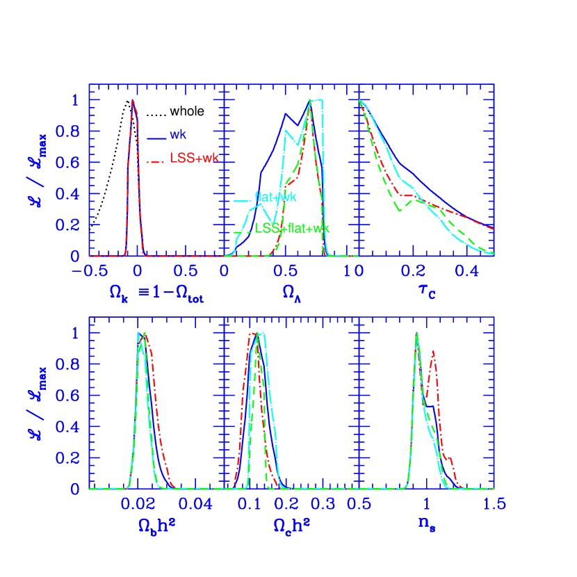
Figure 11.— 1D projected likelihood functions as in Fig. 2, except calculated using all-data (see Table 4).

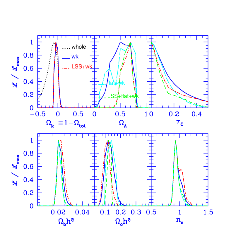
Figure 12.— 1D projected likelihood functions as in Fig. 2, except calculated using CBIo140+DMR+DASI+BOOMERANG+VSA (the data for BOOMERANG are taken from Ruhl et al. 2002).

Table 5all-data

Priors	$\Omega_{\rm tot}$	$n_{s}$	$\Omega_{b}h^{2}$	$\Omega_{\rm cdm}h^{2}$	$\Omega_{\Lambda}$	$\Omega_{m}$	$\Omega_{b}$	$h$	Age	$\tau_{c}$
wk-$h$	$1.04^{0.05}_{0.05}$	$0.98^{0.10}_{0.06}$	$0.023^{0.003}_{0.003}$	$0.12^{0.03}_{0.03}$	$0.55^{0.17}_{0.20}$	$0.49^{0.18}_{0.18}$	$0.075^{0.023}_{0.023}$	$0.56^{0.11}_{0.11}$	$15.1^{1.4}_{1.4}$	$<0.57$
wk-$h$+LSS	$1.04^{0.05}_{0.04}$	$1.01^{0.09}_{0.09}$	$0.023^{0.004}_{0.003}$	$0.11^{0.03}_{0.03}$	$0.66^{0.09}_{0.13}$	$0.39^{0.11}_{0.11}$	$0.069^{0.020}_{0.020}$	$0.60^{0.09}_{0.09}$	$15.2^{1.5}_{1.5}$	$<0.60$
wk-$h$+SN	$1.03^{0.05}_{0.04}$	$1.03^{0.08}_{0.08}$	$0.024^{0.003}_{0.003}$	$0.11^{0.02}_{0.02}$	$0.71^{0.06}_{0.07}$	$0.32^{0.08}_{0.08}$	$0.061^{0.020}_{0.020}$	$0.64^{0.09}_{0.09}$	$14.8^{1.6}_{1.6}$	$<0.63$
wk-$h$+LSS+SN	$1.03^{0.05}_{0.04}$	$1.04^{0.08}_{0.08}$	$0.024^{0.004}_{0.003}$	$0.10^{0.02}_{0.03}$	$0.71^{0.06}_{0.06}$	$0.33^{0.06}_{0.06}$	$0.064^{0.020}_{0.020}$	$0.63^{0.09}_{0.09}$	$15.0^{1.6}_{1.6}$	$<0.63$
flat+wk-$h$	(1.00)	$0.96^{0.09}_{0.05}$	$0.022^{0.003}_{0.002}$	$0.13^{0.03}_{0.03}$	$0.60^{0.15}_{0.26}$	$0.42^{0.20}_{0.20}$	$0.055^{0.015}_{0.015}$	$0.64^{0.11}_{0.11}$	$13.9^{0.5}_{0.5}$	$<0.35$
flat+wk-$h$+LSS	(1.00)	$0.97^{0.09}_{0.05}$	$0.022^{0.003}_{0.002}$	$0.12^{0.02}_{0.02}$	$0.66^{0.09}_{0.12}$	$0.35^{0.10}_{0.10}$	$0.051^{0.008}_{0.008}$	$0.66^{0.08}_{0.08}$	$13.8^{0.5}_{0.5}$	$<0.39$
flat+wk-$h$+SN	(1.00)	$0.99^{0.07}_{0.06}$	$0.023^{0.002}_{0.002}$	$0.12^{0.02}_{0.02}$	$0.71^{0.06}_{0.07}$	$0.29^{0.07}_{0.07}$	$0.045^{0.006}_{0.006}$	$0.71^{0.06}_{0.06}$	$13.6^{0.3}_{0.3}$	$<0.37$
flat+wk-$h$+LSS+SN	(1.00)	$0.99^{0.07}_{0.06}$	$0.023^{0.002}_{0.002}$	$0.12^{0.01}_{0.01}$	$0.70^{0.05}_{0.06}$	$0.30^{0.06}_{0.06}$	$0.047^{0.005}_{0.005}$	$0.69^{0.05}_{0.05}$	$13.7^{0.3}_{0.3}$	$<0.39$
flat+HST-$h$	(1.00)	$0.99^{0.07}_{0.06}$	$0.023^{0.002}_{0.002}$	$0.12^{0.02}_{0.02}$	$0.70^{0.08}_{0.11}$	$0.30^{0.10}_{0.10}$	$0.047^{0.009}_{0.009}$	$0.70^{0.08}_{0.08}$	$13.6^{0.4}_{0.4}$	$<0.37$
flat+HST-$h$+LSS	(1.00)	$0.99^{0.08}_{0.06}$	$0.023^{0.002}_{0.002}$	$0.12^{0.02}_{0.02}$	$0.69^{0.06}_{0.08}$	$0.31^{0.08}_{0.08}$	$0.048^{0.006}_{0.006}$	$0.69^{0.06}_{0.06}$	$13.7^{0.3}_{0.3}$	$<0.39$
flat+HST-$h$+SN	(1.00)	$0.99^{0.07}_{0.05}$	$0.023^{0.002}_{0.002}$	$0.12^{0.01}_{0.02}$	$0.71^{0.06}_{0.05}$	$0.28^{0.06}_{0.06}$	$0.045^{0.006}_{0.006}$	$0.71^{0.05}_{0.05}$	$13.6^{0.2}_{0.2}$	$<0.37$
flat+HST-$h$+LSS+SN	(1.00)	$1.00^{0.06}_{0.05}$	$0.023^{0.002}_{0.002}$	$0.12^{0.01}_{0.01}$	$0.70^{0.05}_{0.05}$	$0.30^{0.05}_{0.05}$	$0.047^{0.004}_{0.004}$	$0.69^{0.04}_{0.04}$	$13.7^{0.2}_{0.2}$	$<0.38$

Note. — Cosmological parameter estimates as in Table 3, but now for all-data.

A full suite of priors for this all-data case is given in Table 5 and the corresponding 1D likelihood plots are shown in Figure 11. Figure 12 shows the small difference when we use BOOMERANG+DASI+CBIo140+DMR. These combined data yield parameters consistent with those derived individually: the curvature is close to flat, the spectral index is close to unity, and the baryon density is near that favoured by Big Bang nucleosynthesis, $\omega_{b}=0.019\pm 0.002$ (Olive et al., 1999; Burles et al., 2000; Tytler et al., 2000).

The tables also show estimates for what we term “derived” parameters. These are parameters that can be expressed as functions of our ${\cal C}_{\ell}$-database parameters. The combinations are $\Omega_{m}$, $\Omega_{b}$, $h$, and the cosmological age $t_{0}$. We calculate the means and variances of these functions over the full probability distribution. We have also applied the same method to the computation of the statistics of $\ell_{{\rm pk},j}$, ${\cal C}_{{\rm pk},j}$, and $\ell_{{\rm dip},j}$, ${\cal C}_{{\rm dip},j}$, and the position and amplitude of the $j$th peak and $j$th dip in ${\cal C}_{\ell}$. These are discussed in detail in the following section (§ 7) and the results from the application to the mosaic data are shown in Paper III. We also determine the values of $\Omega_{m}h$, $\Gamma$,and $\Gamma_{\rm eff}$ in a similar fashion, as reported in Paper VI. Paper VI also reports on calculations of alternate amplitude parameters to ${\cal C}_{10}$, in particular for the $\sigma_{8}$ amplitude used in the LSS prior.

The results set out in the tables also show how applying the prior restrictions LSS, SNIa, or HST-$h$ to the CMB data gives compatible results.

7. Reheating, Recombination, and Damping

In this section, we summarize the basic physical effects expected to have an impact on the ${\cal C}_{\ell}$ spectra we observe, working back from now, through the reionization of the universe, § 7.1, and to the critically important regime for CBI observations, recombination. We discuss briefly the history of computations of the anisotropy in § 7.2, but our main goal is to use the parameters of our best-fit cosmological models to evaluate the physical and multipole scales characterizing the decoupling epoch in § 7.3.

7.1. Reheating

We have used the depth to Thomson scattering from a time $t_{1}$ to the present $t_{0}$, $\tau_{C}=\int_{t_{1}}^{t_{0}}c\,dt\,\bar{n}_{e}\sigma_{T}$, as one of our major cosmological parameters, where $\bar{n}_{e}(t)$ is the average electron density, $\sigma_{T}$ is the Thomson cross section and $c$ is the speed of light. If we assume the Universe has been fully ionized below a redshift $z_{\rm reh}$, we have

$$\tau_{C}\sim 0.1(\omega_{b}/0.02)(\omega_{m}/0.15)^{-1/2}((1+z_{\rm reh})/15)^{3/2}.$$ (2)

A minimum value for $z_{\rm reh}$ is $\sim 5$, so $\tau_{C}\gtrsim 0.03$ is expected. The visibility to Thomson scattering is defined by $e^{-\tau_{C}}$. As long as $\tau_{C}$ is not too large, ${\cal C}_{\ell}$ is suppressed by a factor $\exp[-2\tau_{C}]$ on scales smaller than the horizon at $z_{\rm reh}$, and in particular over the regime probed by CBI, BOOMERANG, DASI, MAXIMA, VSA, etc.

The mechanism for reionization is thought to be the overlap of H II regions generated by massive stars housed in the very small, earliest galaxies to form. Other possibilities, e.g., involving particle decays tuned so that $\tau_{C}$ would not be too large, are more exotic and require extra parameters for the theory. We know that the stars must form, but little about the efficiency of forming the first stars. However $z_{\rm reh}$ is necessarily tied to the formation of nonlinear gas structures, hence to the power spectrum of density fluctuations. For the $\Lambda$CDM models preferred by the CMB data, with $n_{s}\sim 1$, this implies $z_{\rm reh}$ should not be much more than 15, hence our expectation is that $\tau_{C}$ should not be much greater than 0.1. Although the $\tau_{C}$ likelihoods of Figs. 11, 12 now fall off nicely beyond 0.2 or so, a limit as strong as this still eludes us. The inability to determine $\tau_{C}$ with higher precision is attributable in part to parameter near-degeneracies (Efstathiou & Bond, 1999). However the fact that we have detected power at large $\ell$ shows that $z_{\rm reh}$ cannot be too big: e.g., although some pregalactic energy injection at $z\sim 50$ is still possible, it now seems unlikely that it could have led to full reionization at such high redshifts.

The late time reheating described above is almost entirely a damping effect associated with photons coming towards us carrying anisotropy information being scattered away from our line of sight. There is a small effect associated with new scattering sources regenerating CMB anisotropies: the reciprocal effect of photons being scattering into our line of sight does not appreciably add to the anisotropy we observe, so the net effect is the damping decline $\propto e^{-\tau_{C}}$. The differential visibility ${\cal V}_{C}\equiv de^{-\tau_{C}}/d\ln a=e^{-\tau_{C}}\bar{n}_{e}\sigma_{T}/H(z)$, where $H(z)$ is the Hubble parameter at redshift $z$ and $a=(1+z)^{-1}$ is the expansion factor, defines the dominant regions in redshift where the scattering leads to “visible” consequences. Reionization results in a bump in ${\cal V}_{C}$ around $z_{\rm reh}$ with a tail to lower redshift.

7.2. Anisotropies from the Recombination Epoch

We now turn to effects associated with the recombination of the primordial plasma. The essential ingredients were worked out immediately after the discovery of the CMB (Peebles, 1968; Zeldovich, Kurt & Sunyaev, 1969). The novel features are the dominant roles played by the two-photon decay of the $2s$ state to the $1s$ state and leakage from the Lyman alpha line associated with the expansion of the Universe. Improvements including helium recombination (e.g., Hu et al. 1995) and a more sophisticated treatment of hydrogen recombination were essential for the high precision era we are entering now (Seager, Sasselov, & Scott, 1999).

The great simplification afforded by the smallness of the primary anisotropies is that linear perturbation theory can be used and the photon transport equations can be decomposed into independent modes characterized by a comoving wavenumber $k$. Each mode contributes to ${\cal C}_{\ell}$. However, as mentioned in § 1, the transport of the photons through recombination involves all of the complications of radiative transfer as one passes from an optically thick to an optically thin “Thomson scattering atmosphere,” compounded by a changing gravitational potential.

Many attempts have been made, in the long history of CMB, to deconstruct CMB anisotropies into components associated with baryon-photon acoustic compressions and rarefactions, the Doppler effect, damping, finite decoupling surface width, polarization development, and post-decoupling free-streaming propagation. These have included analytic, semi-analytic, and various small-angle and large-angle approaches. There were usually two goals: first and foremost to understand the physics defining the basic features of the spectra; secondly to make quantitative numerical estimations appropriate for the computer power of the times. Some used photon-baryon one-fluid or two-fluid approximations (e.g., Silk 1968; Weinberg 1971; Press & Vishniac 1980; Bonometto, Lucchin & Valdarnini 1984; Bond 1988; Doroshkevich 1988; Starobinsky 1988; Doroshkevich et al. 1988; Seljak 1994; Hu & Sugiyama 1995; Bond 1996; Hu & White 1996); others used these methods in conjunction with other transport approximations, (e.g., Bardeen 1968 (unpublished), Peebles & Yu 1970; Doroshkevich, Zeldovich & Sunyaev 1978; Wilson & Silk 1981; Wilson 1983; Kaiser 1983; Bond & Efstathiou 1984; Vittorio & Silk 1984; Bond & Efstathiou 1987; Jungman et al. 1996; Weinberg 2001a, b; Kaplinghat, Knox & Skordis 2002).

Given the mutual interdependence of the effects, the semi-analytic methods can only be taken so far, and numerical computation of spectra is the preferred method for this high precision era of CMB observations. There were many groups who developed codes to solve the perturbed Boltzmann–Einstein equations when dark matter was present prior to and following shortly after the COBE discovery (Bond & Efstathiou, 1984, 1987; Vittorio & Silk, 1984, 1992; Efstathiou & Bond, 1986; Fukugita et al., 1990; Gouda et al., 1991; Gorski, Stompor & Juszkiewicz, 1993; Crittenden et al., 1993, 1993b; Dodelson & Jubas, 1994; Bond, 1996; Knox, 1995; Hu et al., 1995). Most of these solved hierarchies of coupled multipole equations. A speedy, publicly available and widely used code for evaluation of anisotropies in a variety of cosmological scenarios, “CMBfast” (Seljak & Zaldarriaga, 1996), using line-of-sight past history integrations of CMB anisotropy source terms, has come to dominate the scene, used even by those who developed their own codes and was checked in detail with a number of these other transport codes. It has also had extensions to more cosmological models added by a variety of researchers. Another fast code, “CAMB” (Lewis, Challinor, & Lasenby, 2000), is based on this technique. A suitably modified CMBfast was used in the construction of the ${\cal C}_{\ell}$-database used in Lange et al. (2001) and in this paper.

7.3. Numerology of Recombination and Damping

We have seen that analytic, semi-analytic and deconstruction attempts have been historically important in quantitative CMB work and continue to be qualitatively useful in understanding how the various effects manifest themselves in ${\cal C}_{\ell}$. Here we shall concentrate on some of the scales of relevance for this qualitative description (Bond, 1996; Hu & Sugiyama, 1995; Hu & White, 1996; Efstathiou & Bond, 1999).

As we take $t_{1}$ through photon decoupling and recombination, $\tau_{C}(t_{1})$ grows to extreme opaqueness above the redshift $z_{\rm dec}$ where photons decouple, and where recombination predominantly occurs. The differential visibility ${\cal V}_{C}$ is sharply peaked for normal recombination and only weakly dependent on cosmological parameters. $z_{\rm dec}$ is defined to be where ${\cal V}_{C}$ has a peak. A value $\sim 1100$ is obtained for a wide range of cosmologies. For the $\Omega_{\rm tot}=1$ $\Lambda$CDM cosmologies favored by our CMB data, $z_{\rm dec}\approx 1050$, with age $t_{\rm dec}\approx 400000$ yr, (comoving) “horizon” scale $c\tau_{\rm dec}\sim 110\,\omega_{m}^{-1/2}\,{\rm Mpc}$, and (comoving) distance from us $\chi_{\rm dec}\approx 0.88\,(6000\,\omega_{m}^{-1/2}\,{\rm Mpc})$. (For Einstein de Sitter universes, the 0.88 becomes 0.97.)

The ratio of the density of ordinary matter to relativistic matter at $z_{\rm dec}$ would then be $\sim 3.3$, and the baryon to photon density ratio would be $\sim 0.8$. The sound speed at decoupling, $c_{s}=(c/\sqrt{3})[1+3\bar{\rho}_{B}/(4\bar{\rho}_{\gamma})]^{-1/2}$ is lowered over the $c/\sqrt{3}$ for a pure photon gas because of the inertia in the baryons; for $\omega_{b}=0.02$, it is $\approx 0.8c/\sqrt{3}$, leading to a sound crossing distance $c_{s}\tau_{\rm dec}\approx 50\,\omega_{m}^{-1/2}\,{\rm Mpc}$. Since $c_{s}$ varies with time, an appropriate average $\bar{c}_{s}$ should be used, resulting in an adjustment upward of 12%. The phase of the waves as they hit the narrow recombination band, $k\bar{c}_{s}\tau_{\rm dec}$, determines the oscillations in ${\cal C}_{\ell}$, associating peak $m$ with a length scale $\sim(\bar{c}_{s}\tau_{\rm dec})/(m\pi)$.

To convert the comoving distances at $z_{\rm dec}$ to angular scales, we divide by $\chi_{\rm dec}$. The component of a wavenumber perpendicular to the decoupling surface, $k_{\perp}$ is associated with a multipole $\ell$, where $k_{\perp}^{-1}=\chi_{\rm dec}\ell^{-1}$, $\approx 5.3(1000/\ell)\,\omega_{m}^{-1/2}\,{\rm Mpc}$ for our $\Lambda$ CDM case. The mass in matter enclosed within a perturbation of radius $r$ is $M=2.76\times 10^{11}\omega_{m}(4\pi/3)r^{3}\,{\rm M}_{\odot}$. The appropriate top hat radius of a collapsed object that forms from waves associated with a band about $k$ is $r\sim 2k^{-1}$ (Bond & Myers, 1996). This gives a rich cluster mass, $1.3\times 10^{15}\,\omega_{m}^{-1/2}(1000/\ell)^{3}\,{\rm M}_{\odot}$, for $\ell\sim 1500$.

Converting peaks in $k$-space into peaks in $\ell$-space is obscured by projection effects and the influence of other sources such as the Doppler term. The conversion of the oscillations into peak locations in ${\cal C}_{\ell}$ gives $\ell_{pk,m}\sim f_{m}m\pi\chi_{\rm dec}/(\bar{c}_{s}\tau_{\rm dec})$, where the numerically estimated $f_{m}$ factor is $\approx 0.75$ for the first peak, approaching unity for higher ones. These numbers accord reasonably well with the values we obtain when we average over the probability distribution for our ${\cal C}_{\ell}$-database. Using all-data, and the flat+wk-$h$+LSS prior, the first five peak locations are at $221\pm 2$, $536\pm 5$, $814\pm 17$, $1129\pm 18$, $1427\pm 20$. The interleaving dips are at $413\pm 4$, $673\pm 8$, $1015\pm 10$, $1310\pm 14$, similar to the predicted $(m+1/2)$ spacing. For all-data and the wk-$h$ prior, the positions are very similar, but as expected the errors are slightly larger. We saw in Paper III that the “model-independent” estimation of peak positions from the data accord reasonably well with these ${\cal C}_{\ell}$-database determinations.

The electron density falls dramatically through decoupling: the local power law index, $p=-d\ln n_{e}/d\ln a$, rises from its low and high $z$ asymptotic values of 3 to a maximum of about 15, with 10 to 14 typical at $z_{\rm dec}$, the range depending upon the model; e.g., for $\Lambda$CDM, $p\approx 12$. A “Gaussian” width of decoupling in $\ln a/a_{\rm dec}$ can be estimated analytically from $p$: $\sigma_{a,\rm dec}\approx(p-1)^{-1}$ (apart from a small correction factor associated with the change of $p$). For $\Lambda$CDM, $\sigma_{a,\rm dec}\approx 0.08$. (Although the distribution is somewhat skewed, a Gaussian fit to ${\cal V}_{C}$ turns out to be a reasonably good approximation over the dominant range, and estimating $\sigma_{a,\rm dec}$ from the FWHM of exactly ${\cal V}_{C}$ yields 0.06 to 0.1 in good accord with the analytic estimates.) The corresponding comoving length scale, $R_{C,dec}\approx\sigma_{a,\rm dec}[H(z_{\rm dec})a_{\rm dec}]^{-1}$, is $\sim 7\,\omega_{m}^{-1/2}\,{\rm Mpc}$ for $\Lambda$CDM, to be compared with $c_{s}\tau_{\rm dec}$. Because this is parallel to the line of sight, $R_{C,\rm dec}$ does not project onto an angular scale we can observe, but perpendicular components of this characteristic size would have $\ell\sim 820$.

A combination of viscous (Silk) damping and fuzziness damping diminishes the amplitude of the acoustic peaks. The two effects occur simultaneously, intertwined by the complexities of the transport, but are estimated differently.

Earlier than decoupling, the photons and baryons are so tightly coupled by Thomson scattering that they can be treated as a single fluid with sound speed $c_{s}$, shear viscosity $({4}/(15f_{\eta}))\bar{\rho}_{\gamma}/(n_{e}\sigma_{T})$, zero bulk viscosity, and thermal conductivity $\kappa_{\gamma}=(4\rho_{\gamma}/(3T_{\gamma}))/(n_{e}\sigma_{T})$. Here $f_{\eta}$ is $3/4$ if Thomson scattering is fully treated and 1 if polarization and the angular dependence of the Thomson cross section are ignored. Silk damping has usually been estimated using a WKB approximation to these one-fluid equations, which results in an overall damping multiplier of form $e^{-(k\sigma_{D}\tau_{\rm dec})^{2}/2}$ for $z>z_{\rm dec}$ multiplying the $kc_{s}\tau_{\rm dec}$ terms which give the acoustic oscillations. The parameter $\sigma_{D}$ is an integral of the damping rate involving the shear viscosity and thermal conductivity,

$$\sigma_{D}^{2} \approx {1\over(p-1)(p-1/2)(15f_{\eta})(1+R)}$$

$$+{R^{2}\over(p-1)(p-1/2)12(1+R)^{2}},$$

$$R \equiv {3\bar{\rho}_{B}\over 4\bar{\rho}_{\gamma}}.$$ (3)

With $f_{\eta}=3/4$ and $10\lesssim p\lesssim 14$, we have $0.02\lesssim\sigma_{D}\lesssim 0.03$ over a wide range of cosmological parameters, 0.023 for $\Lambda$CDM, with only a weak sensitivity to $\omega_{b}$. The first term is from shear viscosity, the second is from thermal conductivity. For $\Lambda$CDM with $\omega_{b}=0.02$, the ratio is 5 to 1. Although polarization increases $\sigma_{D}$ by 10%, we cannot determine the damping scale with such accuracy with the CBI data.

For this $\sigma_{D}$, we get $\sigma_{D}c\tau_{\rm dec}\approx 2.4\,\omega_{m}^{-1/2}\,{\rm Mpc}$, giving a scale $\ell_{D}\sim 2160$. However, the tight coupling equations break down as the radiation passes through decoupling, so it is better to treat $\sigma_{D}$ as a phenomenological factor and match it to numerical results. An estimate of the Silk damping scale (given as well by Bond 1996) was $k_{\rm Silk}^{-1}\approx 3.8\,\omega_{m}^{-1/2}\,{\rm Mpc}$, with angular size $2.5^{\prime}$ and $\ell_{\rm Silk}\approx 1390$. A more sophisticated phenomenology of numerical ${\cal C}_{\ell}$-results adopted damping envelope functions, $\exp[-(\ell/\ell_{D})^{m_{D}}]$, multiplying “undamped ${\cal C}_{\ell}$’s” and provided fitting formulas for $\ell_{D}$ and $m_{D}$ (Hu & White, 1996). For the $\Lambda$CDM parameters used here, we get $\ell_{D}=1345$, with a power $m_{D}=1.26$, in good accord with the $\ell_{\rm Silk}$ estimate. Note that the falloff is not as steep as the WKB Gaussian would predict. When we average $\ell_{D}$ over the database, we get $1352\pm 15$ for all-data and the flat+wk-$h$+LSS prior.

The fuzziness damping acts only on $k_{\parallel}$, the component of the waves through the decoupling surface: destructive interference from both peaks and troughs occurs for waves with $k_{\parallel}R_{C,dec}>\pi$, but there is none if the photons are only received from either peaks or troughs, but not both, the case if oscillations are along the surface, or if the wavenumbers are small. (The WKB tight-coupling solution does in fact calculate a version of fuzziness damping along with other transport effects, but the $k_{\perp}$–$k_{\parallel}$ asymmetry is obscured by the truncation of the $\ell$-hierarchy at such low $\ell$: up to $\approx\tau_{\rm dec}$, higher moments are strongly damped, but this is not correct as the photons pass through $z_{\rm dec}$.) In the Gaussian approximation to ${\cal V}_{C}$, fuzziness damping acts on $\Delta T/T$ through a multiplier $e^{-(k_{\parallel}R_{C,dec})^{2}/2}$. Because it acts asymmetrically, it is not as dramatic a drop as in the WKB case even though $R_{C,dec}$ is bigger than $k_{\rm Silk}^{-1}$. A simple estimate of a fuzziness damping scale angle-averages $(k_{\parallel}R_{C,dec})^{2}$, reducing the effective filter to $R_{C,dec}/\sqrt{3}$, giving $\ell_{C,dec}\sim 1420$, similar to $\ell_{\rm Silk}$ and $\ell_{D}$.

If we use $\ell_{D}=1345$ and the damping envelope to “correct” the heights of the peaks and dips determined along with their $\ell$-space locations, the peak power bounces between 4000 and 2500 $\mu\rm K^{2}$ (except for the first peak), and the dip power between 2600 and 1400, “correcting” for a significant fraction of the factor of about five raw variations. It is certainly an attractive proposition to directly translate the CMB data into accurate determination of the physical scales operating at decoupling. However, the intertwining of transport effects makes the use of a parameterized ${\cal C}_{\ell}$ model space a more robust proposition.

8. Conclusions

The CBI provides a unique view of the CMB spectrum extending to much higher $\ell$ than previous experiments which have detected primary anisotropies, and well into the multipole region of the spectrum dominated by the damping of fluctuations at decoupling due to viscosity in the photon-baryon fluid and the finite thickness of the last scattering region. The CBI observations indicate a flat universe with a scale-invariant primordial fluctuation spectrum consistent with the inflationary model; and in addition they indicate a low matter density, a baryon fraction consistent with Big Bang Nucleosynthesis, a non-zero cosmological constant, and a cosmological age consistent with the ages of the oldest stars in globular clusters.

These results hold for the whole CBI data set, and in addition they hold for a subset of the data restricted to $610<\ell<3500$. These findings are therefore independent of the spectrum over the $\ell$-range of the first and second acoustic peaks, and thus provide independent confirmation of the major results determined by other CMB experiments from observations that span the first two or three acoustic peaks. This independent confirmation of the major results gives much confidence that the key assumptions of minimal inflationary models are correct, especially the assumption that the primordial fluctuation spectrum does not have significant fine structure. If there were significant fine structure, it is extremely unlikely that spectral studies over different $\ell$-ranges would yield the same values of key cosmological parameters. The good agreement with the results from lower $\ell$ also demonstrates that the recombination theory of the simple model is substantially correct.

In more detail: the CBI observations from the first year of observing, when combined with DMR, gives the following key cosmological results, as discussed in § 4. Under the weak-$h$+LSS priors we find $\Omega_{\rm tot}=1.05_{-0.08}^{+0.08}$, and $n_{s}=1.07_{-0.10}^{+0.13}$, consistent with inflationary models; $\Omega_{\rm cdm}h^{2}=0.10_{-0.03}^{+0.04}$, and, in addition, identifying the excess energy density with the cosmological constant, we find $\Omega_{\Lambda}=0.67_{-0.13}^{+0.10}$. When the more restrictive priors, flat+weak-$h$+LSS, are used, we find $\Omega_{\rm cdm}h^{2}=0.11_{-0.02}^{+0.02}$, consistent with large scale structure studies; $\Omega_{b}h^{2}=0.024_{-0.009}^{+0.011}$, consistent with Big Bang Nucleosynthesis; $\Omega_{m}=0.34\pm 0.12$, and $\Omega_{b}=0.057\pm 0.020$, indicating a low matter density universe; $h=0.66_{-0.11}^{+0.11}$, consistent with the recent determinations of the Hubble Constant based on the recently revised Cepheid period-luminosity law; and $t_{0}=14.2_{-1.3}^{+1.3}$ Gyr, consistent with cosmological age estimates based on the oldest stars in globular clusters.

These values for key cosmological parameters are in remarkably good agreement with those determined in other recent CMB experiments. As pointed out above, this is highly significant, since the CBI cosmology is based on a higher $\ell$-range than has previously been used and leverages principally off the damping tail region of the spectrum rather than the first acoustic peak.

Another unique aspect of the 500–3500 $\ell$-range that CBI has probed is that the angular scales correspond to the 3D wavenumbers of structures that collapsed to produce clusters of galaxies, ranging from those with masses as low as $10^{14}M_{\sun}$, to large superclusters with masses $\sim 10^{16}M_{\sun}$. Hence the CBI observations span the whole range of masses from small groups of galaxies to large superclusters. Thus detection of CMB power in this region provides a direct link between the small $\Delta T$ fluctuations at the time of photon decoupling and the nonlinear density amplitudes on those scales today. This provides further strong support for the gravitational instability picture of structure formation.

The CBI, BOOMERANG, DASI, MAXIMA, and VSA observations are consistent with one another over the entire range of overlapping coverage in $\ell$. The consistency between the five data sets, obtained by different experiments using different observation strategies on different parts of the sky, eliminates many sources of systematic error as a potential cause for concern. Figure 10 shows concordance of the different experiments in our minimal-inflation parameter space.

Given the small signal levels that are being studied here, it is remarkable that the agreement between the recent CMB experiments (TOCO, BOOMERANG, CBI, DASI, MAXIMA, and VSA) should be so good. The variety of techniques employed, combined with the extension of the spectrum to high-$\ell$ provided by the CBI data and the high $\ell$-resolution data at low multipoles provided by the BOOMERANG, DASI, MAXIMA, and VSA experiments, makes for a compelling case that both the observations and the cosmological results are robust.

We have not treated several other parameters that could be of relevance to the inflation-based model. In place of $\Lambda$CDM, $Q$CDM is receiving much attention, with $Q$ an ultra-low mass scalar field, often called quintessence, that dominates at late times. Thus $\Omega_{Q}$ replaces $\Omega_{\Lambda}$ and an effective $Q$-dynamics is cast in terms of a mean pressure-to-density ratio $w_{Q}=\bar{p}_{Q}/\bar{\rho}_{Q}$, an effective equation of state (EOS). (The dynamics of $Q$ is more complex than this, since $Q$ is expected to be spatially as well as temporally varying. There is also no good candidate for a theory of $Q$.) For $\Lambda$, $w_{Q}=-1$, but $w_{Q}<-1/3$ would get our patch of the Universe into acceleration. $w_{Q}$ is not well determined by CMB data and we require supernova information to get a useful constraint on it (e.g., Bond et al., 2000a, 2002b). The CMB by itself also is insensitive to the addition of a light massive neutrino (H$\Lambda$CDM models) since there is only a small effect on ${\cal C}_{\ell}$. LSS can add discriminatory power but it simply shifts the result to slightly lower (but still nonzero) $\Omega_{\Lambda}$ (e.g., Bond et al., 2000b; Pogosyan & Starobinsky, 1995).

The influence of a possible gravity-wave component will be explored elsewhere but the main result is that it is also expected to have little effect on the main cosmological parameters presented here. It certainly would have no impact on the angular scales probed by CBI.

Although our results show a tantalizing drop in the $\tau_{C}$ likelihood beyond 0.2, as described in § 7,there is some distance to go to get a detection at the $\sim 0.1$ values simple theoretical predictions give for $\Lambda$CDM. Significant early energy injection in the medium cannot have occurred. This constrains a number of possible, if not probable, scenarios: it is always possible to generate many ionizing stars early by amplifying structure formation from rare collapses that occurred at high redshift, having a non-Gaussian component at small masses, or making the primordial spectrum bluer on small scales.

The dominant feature of the CBI data is the overall decline in the power with increasing $\ell$, a strong prediction of the basic theory of photon decoupling, with a damping scale now moderately well determined, as described in § 7. The way the simplest inflation-based models have survived the dramatic extension to higher $\ell$ over what previous experiments probed is rather amazing. As well CBI has provided further evidence that the peaks and dips associated with acoustic oscillations continue to higher $\ell$ and are in roughly the right locations given by the emerging $\Lambda$CDM concordance model. Thus, the CMB results from the CBI and from the BOOMERANG, DASI, MAXIMA, and VSA experiments, both in isolation and particularly in combination, strongly support the chief predictions of the inflation paradigm — the geometry of the universe is flat, the initial density perturbations are nearly scale-invariant, and the density of mass-energy in the universe is dominated by a form other than ordinary matter. Simple models in which structure formation is driven by topological defects are difficult to reconcile with the CMB observations. These conclusions are considerably strengthened by the inclusion of other cosmological results such as measurements of the Hubble constant, the amplitude and shape of the power spectrum, and the accelerating expansion rate. These all point towards a nonzero cosmological constant.

Appendix A Testing the Offset Lognormal Approximation to the Likelihood

Whether we are interested in estimating parameters which are cosmological or those defining an optimal spectrum, the full likelihood surface is required, not just its Gaussian approximation which is valid only in the immediate neighborhood of the maximum. This can in principle only be done by full calculation, though in practice there are two analytic approximations that have have been shown to fit the one-point distributions quite well in all the cases tried (Bond, Jaffe & Knox, 2000; Netterfield et al., 2002). We show these work well for the CBI deep and mosaic cases too in Figures 13 and 14. The simplest and most often used analytic form is the “offset lognormal” distribution. This is obtained by taking a Gaussian in the variable $z^{B}=\ln(q^{B}+q_{Nt}^{B})$, where the offset $q_{Nt}^{B}$ is the effective noise in the experiment:

$${\cal P}(q)\propto\exp[-{\textstyle{1\over 2}}\sum_{BB^{\prime}}(z-\bar{z})^{B}{\cal F}^{(z)}_{BB^{\prime}}(z-\bar{z})^{B^{\prime}}],$$

$${\cal F}^{(z)}_{BB^{\prime}}=(\bar{q}^{B}+q_{\rm Nt}^{B}){\cal F}^{(q)}_{BB^{\prime}}(\bar{q}^{B^{\prime}}+q_{\rm Nt}^{B^{\prime}}).$$ (A1)

Here ${\cal F}^{(q)}_{BB^{\prime}}$ is the curvature matrix for the bandpowers $q^{B}$ and ${\cal F}^{(z)}_{BB^{\prime}}$ is its local transformation to the $z^{B}$ variables. We sometimes use the ensemble average value of ${\cal F}^{(q)}_{BB^{\prime}}$, which is the Fisher matrix, rather than the curvature matrix. Other approaches for evaluating $q_{Nt}^{B}$ are reviewed by Bond & Crittenden (2001). Figures 13 and  14 show how the offset lognormal approximation provides an accurate description of the likelihood in individual bands for both deep and mosaic data to beyond the $2\sigma$ level. It is also evident that the Gaussian and pure lognormal approximations do not fit the likelihoods as well, the former working best in low signal-to-noise bands, the latter in high signal-to-noise bands.

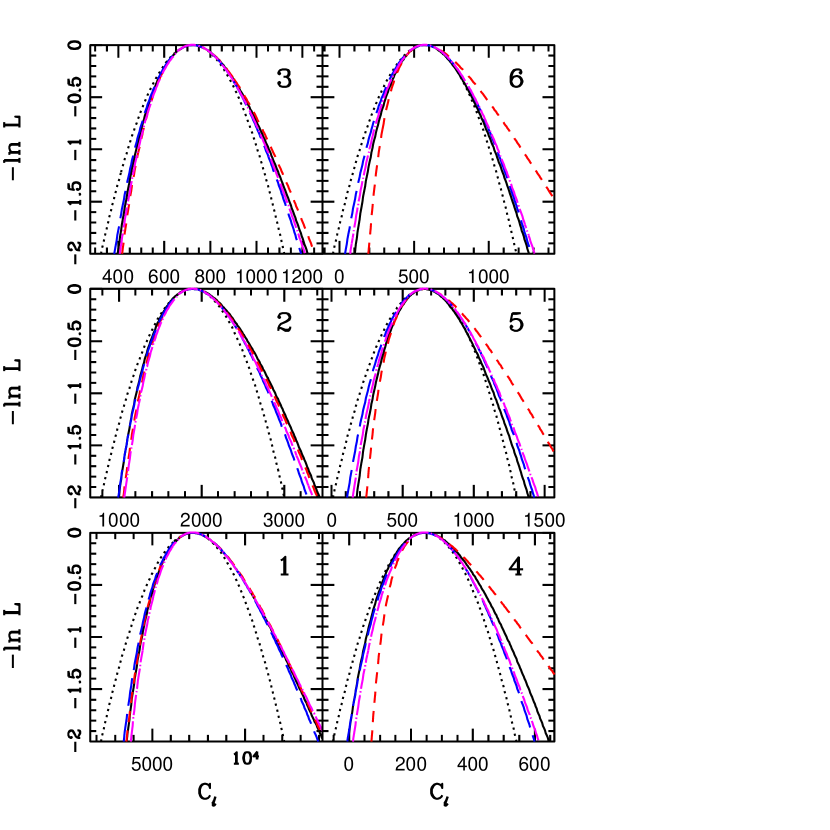
Figure 13.— This shows how well the offset lognormal approximation (long-dashed dark blue) does in reproducing the likelihood functions (solid black) for individual bandpowers $q^{B}$ when the rest of them are fixed at their maximum likelihood values. This is for the first 6 of the 7 CBIdeep bands. The offset logormal approximation with $q_{\rm Nt}^{B}$ determined from our CBI-pipeline reproduces the likelihood function quite well to beyond 2-$\sigma$. Gaussian (dotted black) and log-normal (short-dashed red) distributions are shown for comparison, the former a better fit in the noise-dominated bands, the latter in the cosmic variance dominated bands. The offset log-normal interpolates nicely between the two regimes. The equal-variance approximation (dash-dotted magenta) (Bond, Jaffe & Knox, 2000) also fits quite well. This result is a cornerstone of parameter estimation, whether it be for optimal spectrum combinations of parameterized ${\cal C}_{\ell}$ shapes or for cosmological parameter estimations in a ${\cal C}_{\ell}$-database.

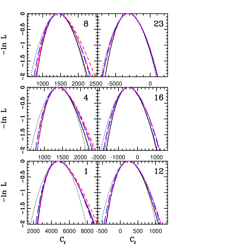
Figure 14.— Same as Fig. 13, but for a selected spread of CBIo140 bands showing again that the offset lognormal approximation works quite well for the CBI mosaic data. Another necessary ingredient is that the bands must not be so closely spaced that the band-to-band correlation as estimated by the inverse Fisher matrix is strong since a weak approximation is used for this band-to-band coupling. Both the $\Delta\ell=140$ and $\Delta\ell=200$ binnings are adequate choices, and deliver similar parameter determinations.

To compare a given theory with spectrum ${\cal C}_{T\ell}(y^{a})$ with the data using equation (A1), the model $q^{B}$’s need to be evaluated with a specific choice for $\varphi_{B\ell}$:

$$q_{B}={\cal I}[{\cal C}_{\ell}\varphi_{B\ell}]/{\cal I}[{\cal C}^{(s)}_{\ell}\varphi_{B\ell}],\ {\rm where}\ {\cal I}[f_{\ell}]\equiv\sum_{\ell}f_{\ell}{\ell+{\textstyle{1\over 2}}\over\ell(\ell+1)}$$ (A2)

is the discrete “logarithmic integral” of a function $f_{\ell}$. The associated bandpower in $(\mu{\rm K})^{2}$ is

$${\cal C}_{B}=q^{B}{\cal C}^{(s)}_{B}\,({\rm no\,sum}),\ {\cal C}^{(s)}_{B}\equiv{\cal I}[{\cal C}^{(s)}_{\ell}\varphi_{B\ell}]/{\cal I}[\varphi_{B\ell}]\,.$$ (A3)

As discussed by Bond, Jaffe & Knox (2000), Knox (1999), and Bond & Crittenden (2001), the window function $\varphi_{B\ell}$ used for this purpose (and therefore with a different notation than the $\psi_{b\ell}$ defined above) is somewhat arbitrary. The simplest choice is again that of a top hat $\chi_{b}(\ell)$. We prefer to use the signal-to-noise windows $W_{B}(\ell)$ derived from the experiment (Paper IV). We have also considered the truncated form $W_{B}(\ell)\chi_{B\ell}$. We find that the cosmological parameters we derive in § 4 and § 6 are insensitive to which form we use. (For example, the largest change occurs in $\omega_{b}$, by 4% in the mean and 10% in the error. This is also evident from Figure 8, which uses $\varphi_{B\ell}=W_{B\ell}$ for the data to create an optimal spectrum with $\psi_{B\ell}=\chi_{B\ell}$; the results are almost identical to the original data.)

If we decrease the width $\Delta\ell$ of bins, we develop more correlation between neighboring bands. The offset lognormal approximation has only been shown to give a good fit when considering individual bins. We therefore require weak band-to-band coupling. We have carried out extensive tests on the dependence of the parameter determinations on binning width and positioning. We showed in § 4 that the inferred cosmologies are insensitive to the choice of bin boundaries.

References

- Allen et al. (1997) Allen, B., Caldwell, R. R., Dodelson, S., Knox, L., Shellard, E. P. S., & Stebbins, A. 1997, Phys. Rev. Lett., 79, 2624
- Doroshkevich et al. (1988) Atrio-Barandela, F., Doroshkevich, A. G., & Klypin, A. A. 1991 ApJ, 378, 1
- Bacon et al. (2002) Bacon, D., Massey, R., Refregier, A., & Ellis, R. 2002, MNRAS, submitted (astro-ph/0203134).
- Bennett (1996) Bennett, C., et al. 1996, ApJ, 464, L1
- Bond (1988) Bond, J. R. 1988, in The Early Universe (Proc. NATO Summer School) ed. W. G. Unruh (Dordrecht: Reidel)
- Bond (1996) Bond, J. R. 1996, in Cosmology and Large Scale Structure, Les Houches Session LX, ed. R. Schaeffer et al. (Elsevier), 469
- Bond & Crittenden (2001) Bond, J. R., & Crittenden, R. G. 2001, in Proc. NATO ASI, Structure Formation in the Universe, ed. R. G. Crittenden & N. G. Turok (Kluwer), in press (astro-ph/0108204)
- Bond & Efstathiou (1984) Bond, J. R. & Efstathiou, G. 1984, ApJ, 285, L45
- Bond & Efstathiou (1987) Bond, J. R. & Efstathiou, G. 1987, MNRAS, 226, 665
- Bond, Efstathiou & Tegmark (1997) Bond, J. R., Efstathiou, G., & Tegmark, M. 1997, MNRAS, 291, L33
- Bond & Jaffe (1998) Bond, J. R., & Jaffe, A. 1998, Phil. Trans. R. Soc. London, 357, 57 (astro-ph/9809043)
- Bond, Jaffe & Knox (1998) Bond, J. R., Jaffe, A. H., & Knox, L. 1998, Phys. Rev. D, 57, 2117
- Bond, Jaffe & Knox (2000) Bond, J. R., Jaffe, A. H., & Knox, L. 2000, ApJ, 533, 19
- Bond & Myers (1996) Bond, J. R. & Myers, S. T. 1996, ApJS, 103, 1
- Bond et al. (2000a) Bond, J. R., et al. 2000, in Cosmology and Particle Physics, Proc. CAPP 2000, AIP conference Proceedings, Volume 555,ed. J. Garcia-Bellida, R. Durrer, & M. Shaposhnikov (Washington: American Inst. of Physics), 85 (astro-ph/0011379)
- Bond et al. (2000b) Bond, J. R., et al. 2000, in XIX Conference on Neutrino Physics and Astrophysics, Proc. Neutrino 2000, ed. D. Hallman, J. Law & J. Simpson (Oxford: Elsevier) (astro-ph/0011381)
- Bond et al. (2003) Bond, J. R., et al. 2003, ApJ, submitted (Paper VI, astro-ph/0205386)
- Bond et al. (2002b) Bond, J. R., et al. 2002, Proc. MRST 2002 (AIP), ed., V. Elias, R.J. Epp, R.C. Myers, p.15 (astro-ph/0210007)
- Bonometto, Lucchin & Valdarnini (1984) Bonometto, S. A., Lucchin, F. & Valdarnini, R. 1984, A&A, 140, 27
- Burles et al. (2000) Brles, S., Nollett, K., Truran, J., & Turner, M. S. 1999, Phys. Rev. Lett., 82, 4176
- de Bernardis et al. (2000) De Bernardis, P., et al. 2000, Nature, 404, 995
- de Bernardis et al. (2002) De Bernardis, P., et al. 2002, ApJ, 564, 559
- Contaldi, Hindmarsh, & Magueijo (1999) Contaldi, C. R., Hindmarsh, M., & Magueijo, J. 1999, Phys. Rev. Lett., 82, 679
- Crittenden et al. (1993) Crittenden, R., Bond, J. R., Davis, R. L., Efstathiou, G. & Steinhardt, P. J. 1993, Phys. Rev. Lett., 71, 324
- Crittenden et al. (1993b) Crittenden, R., Davis, R. & Steinhardt, P. 1993, ApJ, L13
- Dodelson & Jubas (1994) Dodelson, S., & Jubas, J. 1994, Phys. Rev. Lett., 70, 2224
- Doroshkevich (1988) Doroshkevich, A. G. 1988, Pis’ma Zh. Eksp. Teor. Fiz., 14, 296
- Doroshkevich, Zeldovich & Sunyaev (1978) Doroshkevich, A. G., Zeldovich, Ya. B., & Sunyaev, R. A. 1978, Sov. Astron. 22, 523
- Efstathiou & Bond (1986) Efstathiou, G. & Bond, J. R. 1986, MNRAS, 218, 103
- Efstathiou & Bond (1987) Efstathiou, G. & Bond, J. R. 1987, MNRAS, 227, 33P
- Efstathiou & Bond (1999) Efstathiou, G., & Bond, J. R. 1999, MNRAS, 304, 75
- Freedman et al. (2001) Freedman, W. L. 2001, ApJ, 553, 47
- Fukugita et al. (1990) Fukugita, M., Sugiyama, N., & Umemura, M. 1990, ApJ, 358, 28
- Gorski, Stompor & Juszkiewicz (1993) Gorski, K. M., Stompor, R., & Juszkiewicz, R. 1993, ApJ, 410, 1
- Gouda et al. (1991) Gouda, N., Sugiyama, N., & Sasaki, M. 1991, Prog. Theor. Phys., 85, 1023
- Halverson et al. (2002) Halverson, N. W., et al. 2002, ApJ, 568, 38
- Hanany et al. (2001) Hanany, S., et al. 2000, ApJ, 545, L5
- Hoekstra et al. (2002) Hoekstra, H., Yee, H. K. C., & Gladders, M. D. 2002, submitted (astro-ph/0204295).
- Hu et al. (1995) Hu, W., Scott, D., Sugiyama, N., & White, M. 1995, Phys. Rev. D, 52, 5498
- Hu & Sugiyama (1995) Hu, W., & Sugiyama, N. 1995, Phys. Rev. D, 51, 2599
- Hu & White (1996) Hu, W., & White, M. 1996, ApJ, 471, 30
- Jaffe et al. (2001) Jaffe, A. H., et al. 2001, Phys. Rev. Lett., 86, 3475
- Jungman et al. (1996) Jungman, G., Kamionkowski, M., Kosowsky, A. & Spergel, D.N. 1996, Phys. Rev. Lett., 76, 1007
- Kaiser (1983) Kaiser, N. 1983, MNRAS, 202, 1169
- Kaplinghat, Knox & Skordis (2002) Kaplinghat, M., Knox, L., & Skordis, C. 2002, preprint (astro-ph/0203413)
- Kovac et al. (2002) Kovac, J. M., Leitch, E. M., Pryke, C., Carlstrom, J. E., Halverson, N. W., & Holzapfel, W. L. 2002, Nature, 420, 772
- Knox (1995) Knox, L. 1995, Phys. Rev. D, 52, 4307
- Knox (1999) Knox, L. 1999, Phys. Rev. D, 60, 103516
- Lange et al. (2001) Lange, A. E., et al. 2001, Phys. Rev. D, 63, 042001
- Lee et al. (2001) Lee, A. T., et al. 2001, ApJ, 561, L1
- Leitch et al. (2002) Leitch, E. M., Kovac, J. M., Pryke, C., Carlstrom, J. E., Halverson, N. W., Holzapfel, W. L., Dragovan, M., Reddall, B., & Sandberg, E. S. 2002, Nature, 420, 763
- Lewis, Challinor, & Lasenby (2000) Lewis, A., Challinor, A., & Lasenby, A. 2000, ApJ, 538, 473
- Mason et al. (2003) Mason, B. S., et al. 2003, ApJ, in press (Paper II, astro-ph/0205384)
- Mauskopf et al. (2000) Mauskopf, P., et al. 2000, ApJ, 536, L59 (BOOMERANG-NA)
- Miller et al. (1999) Miller, A. D., et al. 1999, ApJ, 524, L1 (TOCO)
- Mould et al. (2000) Mould, J. R., et al. 2000 ApJ, 529, 786
- Myers et al. (2003) Myers, S. T., et al. 2003, ApJ, in press (Paper IV, astro-ph/0205385)
- Netterfield et al. (2002) Netterfield, C. B., et al. 2002, ApJ, in press (preprint astro-ph/0104460)
- Olive et al. (1999) Olive, K. A., Steigman, G., & Walker, T. P. 1999, Phys. Rep., 333, 389
- Peebles (1968) Peebles, P. J. E. 1968, ApJ, 153, 1
- Peebles & Yu (1970) Peebles, P. J. E., & Yu, J.T. 1970, ApJ, 162, 815
- Peacock et al. (2001) Peacock, J. A., et al. 2001, Nature, 410, 169
- Pearson et al. (2003) Pearson, T. J., et al. 2003, ApJ, in press (Paper III, astro-ph/0205388)
- Perlmutter et al. (1999) Perlmutter, S., et al. 1999, ApJ, 517, 565
- Pogosyan & Starobinsky (1995) Pogosyan, D., Starobinsky, A., 1995, ApJ, 447, 465.
- Press & Vishniac (1980) Press, W. H & Vishniac, E. T. 1980, ApJ 236, 323
- Pryke et al. (2002) Pryke, C., et al. 2002, ApJ, 568, 41
- Refregier et al. (2002) Refregier, A., Rhodes, J., & Groth, E. J. 2002, ApJ, submitted (astro-ph/0203131).
- Riess et al. (1998) Riess, A., et al. 1998, AJ, 116, 1009
- Ruhl et al. (2002) Ruhl, J.E., et al. 2002, ApJ, submitted (astro-ph/0212289)
- Scott et al. (2002) Scott, P.F., et al. 2002, MNRAS, submitted (astro-ph/0205380)
- Seager, Sasselov, & Scott (1999) Seager, S., Sasselov, D. D. & Scott, D. 1999, ApJ, 523, L1
- Seljak (1994) Seljak, U. 1994, ApJ, 435, 87
- Seljak & Zaldarriaga (1996) Seljak, U, & Zaldarriaga, M. 1996, ApJ, 469, 437
- Silk (1968) Silk, J. 1968, ApJ, 151, 459
- Starobinsky (1988) Starobinsky, A.A. 1988, Pis’ma Zh. Eksp. Teor. Fiz. 14, 394
- Szalay et al. (2001) Szalay, A. S. et al. 2001, submitted (preprint astro-ph/0107419)
- Turok, Pen, & Seljak (1998) Turok, N., Pen, U., & Seljak, U. 1998, Phys. Rev. D, 58, 3506
- Tytler et al. (2000) Tytler, D., O’Meara, J. M., Suzuki, N., & Lubin, D. 2000, Physica Scripta, submitted (astro-ph/0001318)
- van Waerbeke et al. (2002) Van Waerbeke, L., Mellier, Y., Pello, R., Pen, U.-L., McCracken, H. J., & Jain, B. 2002, A&A, submitted (astro-ph/0202503).
- Vittorio & Silk (1984) Vittorio, N., & Silk, J. 1984, ApJ, 285, L39
- Vittorio & Silk (1992) Vittorio, N., & J. Silk, J. 1992, ApJ, 385, L9
- Weinberg (1971) Weinberg, S. 1971, ApJ, 168, 175
- Weinberg (2001a) Weinberg, S. 2001, Phys. Rev. D, 63, 123511 (astro-ph/0103279)
- Weinberg (2001b) Weinberg, S. 2001, Phys. Rev. D, 64, 123512 (astro-ph/0103281)
- White et al. (1994) White, M., Scott, D., & Silk, J. 1994, ARA&A, 32, 319
- Wilson (1983) Wilson, M. L. 1983, ApJ, 273, 2
- Wilson & Silk (1981) Wilson, M. L., & Silk, J. 1981, ApJ, 243, 14
- Zeldovich, Kurt & Sunyaev (1969) Zeldovich, Ya. B., Kurt, V. G. & Sunyaev, R. A. 1969, Sov. Phys. JETP, 28, 146