A Fast Gridded Method for the Estimation of the Power Spectrum of the CMB from Interferometer Data with Application to the Cosmic Background Imager

Abstract

We describe an algorithm for the extraction of the angular power spectrum of an intensity field, such as the cosmic microwave background (CMB), from interferometer data. This new method, based on the gridding of interferometer visibilities in the aperture plane followed by a maximum likelihood solution for bandpowers, is much faster than direct likelihood analysis of the visibilities, and deals with foreground radio sources, multiple pointings, and differencing. The gridded aperture-plane estimators are also used to construct Wiener-filtered images using the signal and noise covariance matrices used in the likelihood analysis. Results are shown for simulated data. The method has been used to determine the power spectrum of the cosmic microwave background from observations with the Cosmic Background Imager, and the results are given in companion papers.

1 Introduction

The technique of interferometry has been widely used in radio astronomy to image the sky using arrays of antennas. By correlating the complex voltage signals between pairs of antennas, the field-of-view of a single element can be sub-divided into “synthesized beams” of higher angular resolution. In the small-angle approximation, the interferometer forms the Fourier transform of the sky convolved with the autocorrelation of the aperture voltage patterns. In standard radio interferometric data analysis, as described for example in the text by Thompson, Moran, & Swenson (1986) and the proceedings of the NRAO Synthesis Imaging School (Taylor, Carilli, & Perley, 1999), the correlations or visibilities are inverse Fourier transformed back to the image plane. However, there are applications such as estimation of the angular power spectrum of fluctuations in the cosmic microwave background (CMB) where it is the distribution of and correlation between visibilities in the aperture or $uv$-plane that is of most interest.

In standard cosmological models, the CMB is assumed to be a statistically homogeneous Gaussian random field (Bond & Efstathiou, 1987). In this case, the spherical harmonics of the field are independent and the statistical properties are determined by the power spectrum $C_{\ell}$ where $\ell$ labels the component of the Legendre polynomial expansion (and is roughly in inverse radians). Bond & Efstathiou (1987) showed that in cold dark matter inspired cosmological models, there would be features in the CMB power spectrum that reflected critical properties of the cosmology. Recent detections of the first few of these “acoustic peaks” at $\ell<1000$ in the power spectrum (Lange et al., 2001; Hanany et al., 2001; Lee et al., 2001; Halverson et al., 2002; Netterfield et al., 2001) have supported the standard inflationary cosmological model with $\Omega_{tot}\approx 1$. Measurement of the higher-$\ell$ peaks and troughs, as well as the damping tail due to the finite thickness of the last scattering surface, is the next observational step. Interferometers are well-suited to the challenge of mapping out features in the CMB power spectrum, with a given antenna pair probing a characteristic $\ell$ proportional to the baseline length in units of the observing wavelength (a $100\lambda$ projected baseline corresponds to $\ell\sim 628$, see §3).

There are many papers in the literature on the analysis of CMB anisotropy measurements, estimation of power spectra, and the use of interferometry for CMB studies. General issues for analysis of CMB datasets are discussed in Bond, Jaffe, & Knox (1998, 2000). Hobson, Lasenby, & Jones (1995) present a Bayesian method for the analysis of CMB interferometer data, using the 3-element Cosmic Anisotropy Telescope data as a test case. A description of analysis techniques for interferometric observations from the Degree Angular Scale Interferometer (DASI) were presented in White et al. (1999a, b), while Halverson et al. (2002) report on the power spectrum results from first-season of DASI observations. Ng (2001) discusses CMB interferometry with application to the proposed AMIBA instrument. Hobson & Maisinger (2002) have recently presented an approach similar to ours, and demonstrate their technique on simulated Very Small Array (VSA) data; a brief comparison of their algorithm with ours is given in Appendix C.

In this paper, we describe a fast gridded method for the $uv$-plane analysis of large interferometric data sets. The basis of this approach is to grid the visibilities and perform maximum likelihood estimation of the power spectrum on this compressed data. Our use of gridded estimators is significantly different from what has been done previously. In addition to power spectrum extraction, this procedure has the ability to form optimally filtered images from the gridded estimators, and may be of use in interferometric observations of radio sources in general.

We have applied our method to the analysis of data from the Cosmic Background Imager (CBI). The CBI is a planar interferometer array of 13 individual 90-cm Cassegrain antennas on a 6-m pointable platform (Padin et al., 2002). It covers the frequency range 26–36 GHz in 10 contiguous 1 GHz channels, with a thermal noise level of $2\,\mu$K in 6 hours, and a maximum resolution of $4^{\prime}$ limited by the longest baselines. The CBI baselines probe $\ell$ in the range 500–3900. The 90-cm antenna diameters were chosen to maximize sensitivity, but their primary beamwidth of $45\farcm 2$ (FWHM) at 31 GHz limits the instantaneous field of view, which in turn limits the resolution in $\ell$. This loss of aperture plane resolution can be overcome by making mosaic observations, i.e. observations in which a number of adjacent pointings are combined (Ekers & Rots, 1979; Cornwell, 1988; Cornwell, Holdaway, & Uson, 1993; Sault, Staveley-Smith, & Brouw, 1996). In the CBI observations, mosaicing a field several times larger than the primary beam has resulted in an increase in resolution in $\ell$ by more than a factor of 3, sufficient to discern features in the power spectrum.

The first CBI results were presented in Padin et al. (2001), hereafter Paper I, using earlier versions of the software that did not make use of $uv$-plane gridding, and were far too slow to be used on larger mosaiced data sets. It was therefore essential to develop a more efficient analysis method that would be fast enough to carry out extensive tests on the CBI mosaic data. The software package described below has been used to process the first year of CBI data. In the companion papers (Mason et al., 2002, hereafter Paper II) and (Pearson et al., 2002, hereafter Paper III), the results from passing CBI deep-field data and mosaic data respectively through the pipeline are presented. This paper is Paper IV in the series. The output from this pipeline is then used to derive constraints on cosmology (Sievers et al., 2002, hereafter Paper V). Finally, analysis of the excess of power at high-$\ell$ seen in results shown in Paper II in the context of the Sunyaev-Zeldovich effect is carried out, again using the method presented here, in (Bond et al., 2002, hereafter Paper VI).

An introduction to the properties of the CMB power spectrum, the response of an interferometer to the incoming radiation, and the computation of the primary beam are given in sections §2, §3, and §4 respectively. The gridding process is presented in §5, followed by a description of the likelihood function and construction of the various covariance matrices in §6. Details on the maximum likelihood solution and the calculation of window functions and component bandpowers is given in §7, while §8 presents our method for making optimally filtered images from the gridded estimators. Finally, a description of the CBI implementation of this method and the performance of the pipeline, including demonstrations using simulated CBI datasets, is given in §9, followed by a summary and conclusions in §10.

2 The CMB Power Spectrum

At small angles, the curvature of the sky is negligible and we can approximate the spherical harmonic transform of the the temperature field $T(\mbox{\boldmath$x$})$ in direction $x$ as its Fourier transform $\tilde{T}(\mbox{\boldmath$u$})$ (Bond & Efstathiou, 1987), where $u$ is the conjugate variable to $x$. We adopt the Fourier convention

$$\tilde{F}(\mbox{\boldmath$u$})=\int d^{2}\mbox{\boldmath$x$}\,F(\mbox{\boldmath$x$})\,e^{-2\pi i\mbox{\boldmath$\scriptstyle u$}\cdot\mbox{\boldmath$\scriptstyle x$}}\\ \hskip 28.45274pt\Leftrightarrow\hskip 28.45274ptF({\bf x})=\int d^{2}\mbox{\boldmath$u$}\,\tilde{F}(\mbox{\boldmath$u$})\,e^{2\pi i\mbox{\boldmath$\scriptstyle u$}\cdot\mbox{\boldmath$\scriptstyle x$}}$$ (1)

of Bracewell (1986), Thompson, Moran, & Swenson (1986), and Taylor, Carilli, & Perley (1999). In terms of the multipoles $\ell$,

$$\left\langle\tilde{T}(\mbox{\boldmath$u$})^{2}\right\rangle\approx C_{\ell}\hskip 56.9055pt\ell+1/2\approx 2\pi|\mbox{\boldmath$u$}|$$ (2)

which we simplify to $\ell=2\pi|\mbox{\boldmath$u$}|$ for the $\ell>100$ of interest in this paper. For the low levels anisotropy seen in the CMB on these scales, it is convenient to give $T$ in units of $\mu$K and thus $C_{\ell}$ will be in units of $\mu{\rm K}^{2}$.

Because the CMB is assumed to be a statistically homogeneous Gaussian random field, the components of its Fourier transform are independent Gaussian deviates.

$$\left\langle\tilde{T}(\mbox{\boldmath$u$})\,\tilde{T}^{\ast}(\mbox{\boldmath$u$}^{\prime})\right\rangle=C(|\mbox{\boldmath$u$}|)\,\delta^{2}(\mbox{\boldmath$u$}-\mbox{\boldmath$u$}^{\prime})$$ (3)

where $C(|\mbox{\boldmath$u$}|)=C_{2\pi|\mbox{\boldmath$\scriptstyle u$}|}$. Because $T(\mbox{\boldmath$x$})$ is real, its transform must be Hermitian, with $\tilde{T}(\mbox{\boldmath$u$})=\tilde{T}^{\ast}(-\mbox{\boldmath$u$})$, and therefore

$$\left\langle\tilde{T}(\mbox{\boldmath$u$})\,\tilde{T}(\mbox{\boldmath$u$}^{\prime})\right\rangle=\left\langle\tilde{T}(\mbox{\boldmath$u$})\,\tilde{T}^{\ast}(-\mbox{\boldmath$u$}^{\prime})\right\rangle=C(|\mbox{\boldmath$u$}|)\,\delta^{2}(\mbox{\boldmath$u$}+\mbox{\boldmath$u$}^{\prime}).$$ (4)

Note that it is common to write the CMB power spectrum $C_{\ell}$ in a form

$${\cal C}_{\ell}={\ell(\ell+1)\over 2\pi}\,C_{\ell}\approx{\ell^{2}\over 2\pi}\,C_{\ell}\hskip 28.45274pt\Leftrightarrow\hskip 28.45274pt{\cal C}(|\mbox{\boldmath$u$}|)\approx 2\pi\,|\mbox{\boldmath$u$}|^{2}\,C(|\mbox{\boldmath$u$}|)$$ (5)

(White et al., 1999a; Bond, Jaffe, & Knox, 1998, 2000). Constant ${\cal C}$ corresponds to equal power in equal intervals of $\log\ell$.

Although the power spectrum $C_{\ell}$ is defined in units of brightness temperature, the interferometer measurements carry the units of flux density $S_{\nu}$ (Janskys, 1 Jy = $10^{-26}$ W m^-2 Hz^-1). In particular, the intensity field on the sky $I_{\nu}(\mbox{\boldmath$x$})$ has units of specific intensity (W m^-2 Hz^-1 sr^-1 or Jy/sr), and thus to convert between $I_{\nu}$ and $T$ we use $I_{\nu}(\mbox{\boldmath$x$})=f_{\rm T}(\nu)\,T(\mbox{\boldmath$x$})$ with the Planck factor

$$f_{\rm T}(\nu)=2\nu^{2}k_{\rm B}g(\nu,T_{0})/c^{2}\hskip 56.9055ptg(\nu,T_{0})={x^{2}e^{x}\over(e^{x}-1)^{2}}\hskip 56.9055ptx=h\nu/k_{\rm B}T_{0}$$ (6)

where $g$ corrects for the blackbody spectrum. Note that We have treated the temperature $T$ as small fluctuations about the mean CMB temperature $T_{0}=2.725$ K (Mather et al., 1999), and thus the $g$ appropriate to $T_{0}$ is used with $g\approx 0.98$ at $\nu=31$ GHz.

We are not restricted to modeling the CMB. For example, we might wish to determine the power spectrum of fluctuations in a diffuse galactic component such as synchrotron emission or thermal dust emission. In this case, one might wish to express $I$ in Jy/sr, but take out a power-law spectral shape

$$I_{\nu}=f_{0}(\nu)\,I_{0}\hskip 56.9055ptf_{0}(\nu)=\left({\nu\over\nu_{0}}\right)^{\alpha}$$ (7)

where $\alpha$ is the spectral index, and $f_{0}(\nu)$ is the conversion factor that normalizes to the intensity $I_{0}$ at the fiducial frequency $\nu_{0}$. Note that this normalization is particularly useful for fitting out centimeter-wave foreground emission, which tends to have a power-law spectral index in the range $-1<\alpha<1$ that is significantly different from that for the thermal CMB ($\alpha\approx 2$). In addition, foregrounds will also tend to have a power spectrum shape different from that of CMB, which must be included in the analysis (see §6.4 below).

3 Response of the Interferometer

A visibility $V_{k}$ formed from the correlation of an interferometer baseline between two antennas with projected separation (in the plane perpendicular to the source direction) $b$ meters observed at wavelength $\lambda$ meters measures (in the absence of noise) the Fourier transform of the sky intensity modulated by the response of the antennas (Thompson, Moran, & Swenson, 1986)

$$V(\mbox{\boldmath$u$})=\int d^{2}\mbox{\boldmath$x$}\,{\cal A}(\mbox{\boldmath$x$})\,I(\mbox{\boldmath$x$})\,e^{-2\pi i\mbox{\boldmath$\scriptstyle u$}\cdot\mbox{\boldmath$\scriptstyle x$}}\hskip 56.9055pt\mbox{\boldmath$u$}=\mbox{\boldmath$b$}/\lambda$$ (8)

where ${\cal A}(\mbox{\boldmath$x$})$ is the primary beam, and $\mbox{\boldmath$u$}=(u,v)$ is the conjugate variable to $x$. For angular coordinates $x$ in radians, $u$ has the dimensions of the baseline or aperture in units of the wavelength. The Fourier domain is also referred to as the uv-plane or aperture plane in interferometry for this reason.

We define the direction cosines

$$\mbox{\boldmath$x$}_{k}=(\Delta x_{k},\Delta y_{k})\qquad\Delta x_{k} = \cos\delta_{k}\,\sin(\alpha_{k}-\alpha_{0})$$

$$\Delta y_{k} = \sin\delta_{k}\,\cos\delta_{0}-\cos\delta_{k}\,\sin\delta_{0}\,\cos(\alpha_{k}-\alpha_{0})$$ (9)

between the point at right ascension and declination $\alpha_{k},\delta_{k}$ and the center of the mosaic $\alpha_{0},\delta_{0}$. For the CBI, data are taken keeping the phase center fixed on the pointing center $\mbox{\boldmath$x$}_{k}$ by shifting the phase with the beam and rotating the platform to maintain constant parallactic angle during a scan, so that the response to a point source at the center of the field $I(\mbox{\boldmath$x$})=\delta^{2}(\mbox{\boldmath$x$}-\mbox{\boldmath$x$}_{k})$ is constant, and thus

$${\cal A}(\mbox{\boldmath$x$})=A_{k}(\mbox{\boldmath$x$}-\mbox{\boldmath$x$}_{k})\,e^{2\pi i\mbox{\boldmath$\scriptstyle u$}_{k}\cdot\mbox{\boldmath$\scriptstyle x$}_{k}}$$ (10)

in equation (8), where $A_{k}$ is the normalized primary beam response at the observing frequency of visibility $k$. Then, by application of the Fourier shift theorem, it is easy to show that

$$V_{k} = \int d^{2}\mbox{\boldmath$x$}\,A_{k}(\mbox{\boldmath$x$}-\mbox{\boldmath$x$}_{k})\,I_{\nu_{k}}(\mbox{\boldmath$x$})\,e^{-2\pi i\mbox{\boldmath$\scriptstyle u$}_{k}\cdot(\mbox{\boldmath$\scriptstyle x$}-\mbox{\boldmath$\scriptstyle x$}_{k})}+e_{k}$$ (11)

$$= \int d^{2}\mbox{\boldmath$v$}\,\tilde{A}_{k}(\mbox{\boldmath$u$}_{k}-\mbox{\boldmath$v$})\,\tilde{I}_{\nu_{k}}(\mbox{\boldmath$v$})\,e^{2\pi i\mbox{\boldmath$\scriptstyle v$}\cdot\mbox{\boldmath$\scriptstyle x$}_{k}}+e_{k}$$

where $\tilde{A}_{k}$ is the Fourier transform of the primary beam ${A}_{k}$, and $I_{\nu}(\mbox{\boldmath$x$})$ is the sky brightness field (expressed in units such as Jy/sr) with transform $\tilde{I}_{\nu}(\mbox{\boldmath$v$})$. The instrumental noise on the complex visibility measurement is represented by $e_{k}$.

The uv-plane resolution of an interferometer in a single pointing is thus limited by the convolution with $\tilde{A}$. However, these sub-aperture spatial frequencies can be recovered by using the phase gradient in the exponential $\exp\big{[}2\pi i\mbox{\boldmath$v$}\cdot\mbox{\boldmath$x$}_{k}\big{]}$ from a raster of mosaic pointings $\{\mbox{\boldmath$x$}_{k}\}$, provided that the spacing of the pointings is sufficiently small to avoid aliasing as discussed in Appendix A.

To aid us later on, we introduce a convolution kernel

$$P_{k}(\mbox{\boldmath$v$})=f_{k}\,\tilde{A}_{k}(\mbox{\boldmath$u$}_{k}-\mbox{\boldmath$v$})\,e^{2\pi i\mbox{\boldmath$\scriptstyle v$}\cdot\mbox{\boldmath$\scriptstyle x$}_{k}}$$ (12)

and thus

$$V_{k}=\int d^{2}\mbox{\boldmath$v$}\,P_{k}(\mbox{\boldmath$v$})\,\tilde{T}(\mbox{\boldmath$v$})+e_{k}$$ (13)

where $f_{k}=f_{\rm T}(\nu_{k})$ is the Planck conversion factor for the CMB given in equation (6). It is easiest to write these in operator notation, with

$$\mbox{\boldmath$V$}={\bf P}\,\tilde{\mbox{\boldmath$T$}}+\mbox{\boldmath$e$}$$ (14)

where ${\bf V}$ and ${\bf e}$ are the visibility and noise vectors respectively, ${\bf P}$ is our kernel, and $\tilde{\mbox{\boldmath$T$}}$ is the transform of the temperature field. In this representation $\tilde{\mbox{\boldmath$T$}}$ can be thought of as a vector of cells in uv space.

4 The Primary Beam

In order to determine the response of the array to the radiation field, we need to know the primary beam $A(\mbox{\boldmath$x$})$ of the antenna elements and its Fourier transform $\tilde{A}(\mbox{\boldmath$u$})$. In general, for each frequency channel, each baseline has a primary beam which is the Fourier transform of the cross-correlation of the voltage illumination functions across the aperture of each antenna — see Thompson, Moran, & Swenson (1986) for a detailed treatment of the interferometer response. For a real and symmetric primary beam that is identical between antennas, then the transforms are symmetric and real we can ignore the differences between cross-correlation and convolution and write

$$\tilde{A}(\mbox{\boldmath$u$})=\hat{g}\star\hat{g}\Leftrightarrow A(\mbox{\boldmath$x$})=\big{|}\tilde{g}^{2}\big{|}$$ (15)

for the voltage illumination function $\hat{g}(r,\nu)$ across the radius of the aperture $r=|\mbox{\boldmath$r$}|$ at frequency $\nu$, where $\tilde{g}$ is the Fourier transform of $\hat{g}$. The CBI beams have been measured and are nearly identical and symmetric, and thus we will use a single mean primary beam and its transform for the array. For a heterogeneous array, the individual beams can be used with some added complication.

For most antennas, such as those used in the CBI, the primary beam width scales linearly with observing wavelength, and thus $\hat{g}(r)$ is approximately constant with wavelength. Then, we can define $G(r)$ as the normalized aperture autocorrelation function, and write

$$\tilde{A}_{k}(\mbox{\boldmath$u$})={1\over A_{0}}\,G(|\mbox{\boldmath$u$}|\,\lambda_{k})$$ (16)

for a channel centered at wavelength $\lambda_{k}$, with

$$A_{0}=\int d^{2}\mbox{\boldmath$u$}\,G(|\mbox{\boldmath$u$}|\,\lambda_{k})={2\pi\over\lambda_{k}^{2}}\int_{0}^{\infty}r\,dr\,G(r)$$ (17)

normalizes the response to give unity gain on-sky at the beam center ($A(0)\equiv 1$). If $g(r)=\hat{g}(r)/g(0)$, then $G(r)=g\star g$.

The two-dimensional primary beam response, $A(\mbox{\boldmath$x$})$, is determined by means of measurements of a bright radio source over a two-dimensional grid of offset pointings centered on the source. The central lobe of $A(\mbox{\boldmath$x$})$ for the CBI is well approximated by a circular Gaussian, which is characterized by its dispersion $\sigma_{x}$, which is related to the full width at half-maximum (FWHM) $a_{x}$ by $\sigma_{x}=a_{x}/\sqrt{8\,\ln 2}$. The Fourier transform of an infinite circular Gaussian is given by

$$A(\mbox{\boldmath$x$})=e^{-{x^{2}\over 2\sigma_{x}^{2}}}\Leftrightarrow\tilde{A}(\mbox{\boldmath$u$})={1\over 2\pi\sigma_{u}^{2}}\,e^{-{|\mbox{\boldmath$\scriptstyle u$}|^{2}\over 2\sigma_{u}^{2}}}\hskip 56.9055pt\sigma_{u}={1\over 2\pi\sigma_{x}}$$ (18)

where $\sigma_{u}$ is the Gaussian dispersion in Fourier space. The function $G(r)$ is therefore

$$G(r)=e^{-{r^{2}\over 2r_{g}^{2}}}$$ (19)

for Gaussian radius $r_{g}=\lambda\,\sigma_{u}$. For the CBI the measured primary beam (see Paper III) has $a_{x}=45\farcm 2\times(31{\rm GHz}/\nu)$, so $\sigma_{u}=28.50$ at 31 GHz ($\lambda=0.967$ cm), which corresponds to $r_{g}=27.56$ cm.

For the CBI software pipeline, instead of using a Gaussian approximation to $G(r)$ we have chosen to model the antenna illumination $g(r)$ as a Gaussian truncated at both the dish edge and the secondary blockage radius

$$g(r)=\left\{\begin{array}[]{ll}0&|r|\leq r_{\rm inner}\\ e^{-{\left({r\over s}\right)^{2}}}&r_{\rm inner}<|r|<D/2\\ 0&|r|\geq D/2\end{array}\right.$$ (20)

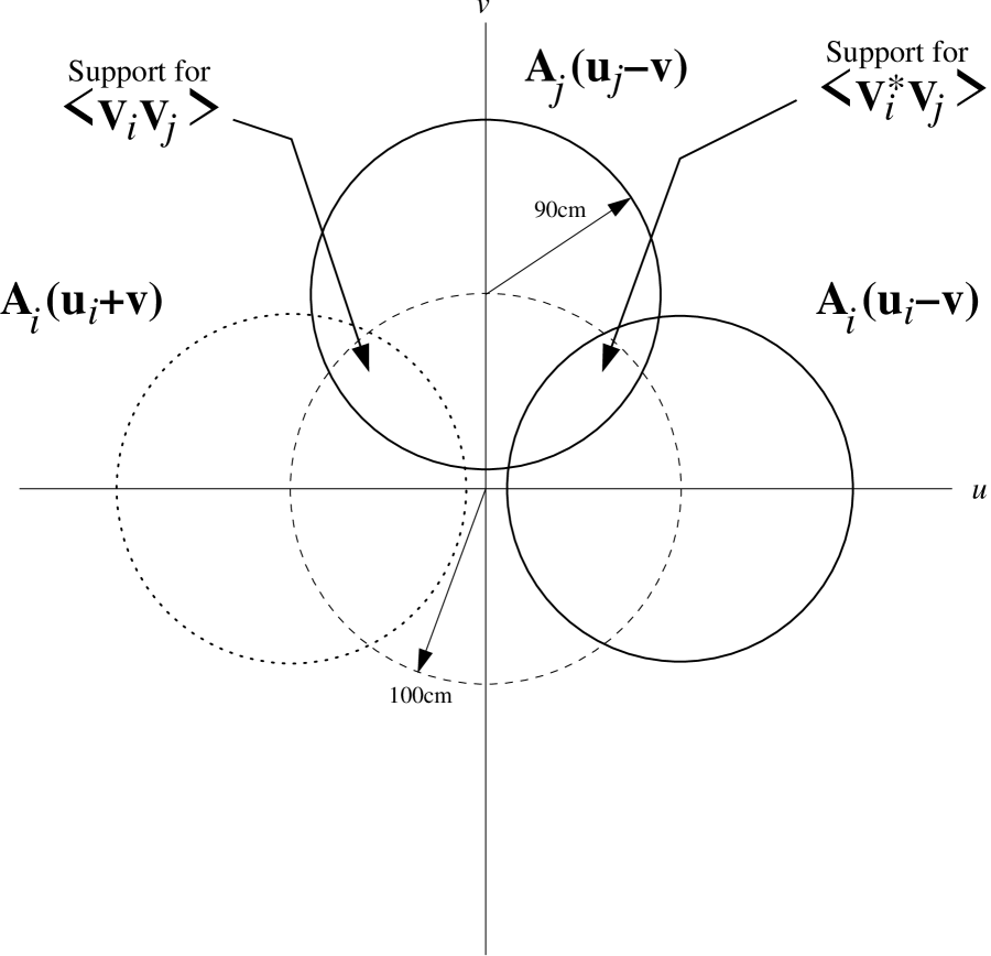
Figure 1: Graphical representation of the regions of support in the aperture plane for the correlation between visibilities on short baselines $B<\sqrt{2}D$. Note that both $V_{i}$ and its conjugate $V^{\ast}_{i}=V(-{\bf u}_{i})$ have overlapping support for visibility $V_{j}$, and this must be taken into account in computing the covariance matrix element.

where for the CBI antennas $r_{\rm inner}=7.75$ cm. Note that if $g(r)$ and $G(r)$ were infinite circular Gaussians, then $s=r_{g}$. A best-fit taper parameter $s$ is obtained using the measured primary beam $A$, giving $s=30.753$ cm or an edge taper of 0.118 ($-18.6$ db of power) at the dish edge. We then numerically tabulate the autocorrelation $G(r)$ assuming $s=30.753$ cm which is then interpolated in the code when $\tilde{A}$ is required. This model is a better fit to the observed beam than a pure Gaussian beam (see Figure 1 in Paper III for a plot of this model).

The resolution in $uv$ or $\ell$ space is set by the width of $\tilde{A}_{k}(\mbox{\boldmath$u$})$. For a Gaussian approximation to the beam, the dispersion in multipole $\ell$ is $\sigma_{\ell}=2\pi\sigma_{u}=1/\sigma_{x}$, and the FWHM is $a_{\ell}=8\,\ln 2/a_{x}$. For $a_{x}=45\farcm 2$ at 31 GHz we have FWHM $a_{\ell}=422$ ($\sigma_{\ell}=179$). Given that features are expected in the power spectrum of widths significantly less than this, it is highly desirable to reduce the effective resolution width of the CBI by at least a factor three using mosaicing.

5 Gridded Estimators

The principal problem in using likelihood (see §6) to determine confidence limits on the power spectrum for CBI data is the large number of visibilities compounded by the large number of mosaic pointings (typically $7\times 6$ or larger). Even a modest reduction in the number of matrix elements passed to the likelihood calculation will greatly aid the computation. This suggests that we grid the visibilities before computing the likelihood function. For an effective resolution in the aperture plane determined by the primary beam and mosaic size, there is little use in sampling below this smearing scale, and we can define an optimum gridding scheme which minimizes the quantity of data and information loss (the gridding is a form of compression).

We implement this by defining estimators $\Delta(\mbox{\boldmath$u$})$ for the true complex brightness transform which are linear combinations of the measured visibilities. These estimators bin together data from the different frequency bands and mosaic pointings. Thus, a direct sum of visibilities taken at the same ${\bf u}$ but over the whole mosaic ${\bf x}$ will result in an estimator that has a higher effective resolution in the uv plane. The result is that we can speed up the likelihood estimation at the cost of complicating the covariance matrix. In general, this matrix can be computed relatively quickly as it is a $N^{2}$ process, and thus this is a worthwhile trade-off versus the $N^{3}$ cost of calculating the likelihood. The estimators derived in Appendix A are not orthogonal combinations of the original visibilities, and thus some information loss is expected. However, the tests performed in §9.1 show that these estimators are unbiased, and comparisons to results obtained using the visibilities directly show that there is no noticeable loss in sensitivity. Thus, our gridding can be considered to be an efficient form of (lossy) compression using the beam as a signal template.

In Appendix A, we argue that a $\Delta_{i}$ formed by a linear combination of visibilities will give a estimate of the weighted average of $\tilde{I}$ or $\tilde{T}$ around uv locus $\mbox{\boldmath$u$}_{i}$. We have from equation (A13)

$$\mbox{\boldmath$\Delta$}={\bf Q}\,\mbox{\boldmath$V$}+\overline{\bf Q}\,\mbox{\boldmath$V$}^{\ast}$$ (21)

where the kernel ${\bf Q}$ is defined in equation (A13) and the kernel for the conjugate visibilities $\overline{\bf Q}$ is defined in equation (A17). In particular,

$$Q_{ik} = {\omega_{k}\over z_{i}}\,\tilde{A}^{\ast}_{k}(\mbox{\boldmath$u$}_{k}-\mbox{\boldmath$u$}_{i})e^{-2\pi i\mbox{\boldmath$\scriptstyle u$}_{i}\cdot\mbox{\boldmath$\scriptstyle x$}_{k}}$$

$$\overline{Q}_{ik} = {\omega_{k}\over z_{i}}\,\tilde{A}^{\ast}_{k}(-\mbox{\boldmath$u$}_{k}-\mbox{\boldmath$u$}_{i})e^{-2\pi i\mbox{\boldmath$\scriptstyle u$}_{i}\cdot\mbox{\boldmath$\scriptstyle x$}_{k}}$$ (22)

where $z_{i}$ the normalization factor given in equation (A21), and $\omega_{k}=\epsilon_{k}^{-2}$ is the visibility weight given in equation (A19).

By operating with the gridding kernel on equation (14), we get

$$\mbox{\boldmath$\Delta$}={\bf R}\,\tilde{\mbox{\boldmath$T$}}+\mbox{\boldmath$n$}\hskip 56.9055pt{\bf R}={\bf Q}\,{\bf P}+\overline{\bf Q}\,\overline{\bf P}\hskip 56.9055pt\mbox{\boldmath$n$}={\bf Q}\,\mbox{\boldmath$e$}+\overline{\bf Q}\,\mbox{\boldmath$e$}^{\ast}$$ (23)

where we define ${\bf R}$ as the convolution kernel that operates on the transform of the intensity (the gridded version of ${\bf P}$), and $n$ is the gridded noise. The conjugate to ${\bf P}$ defined in equation (12) is given by

$$\overline{P}_{k}(\mbox{\boldmath$v$})=f_{k}\,\tilde{A}_{k}(-\mbox{\boldmath$u$}_{k}-\mbox{\boldmath$v$})\,e^{2\pi i\mbox{\boldmath$\scriptstyle v$}\cdot\mbox{\boldmath$\scriptstyle x$}_{k}},$$ (24)

which gathers the conjugate visibilities under the transformation $\mbox{\boldmath$u$}_{k}\rightarrow-\mbox{\boldmath$u$}_{k}$.

Although it is not necessary to do so, it is convenient to construct the $\Delta_{i}$ on a regular lattice in $\mbox{\boldmath$u$}_{i}$ with a spacing $d_{u}$. Thus the grid “cells” represented by the $\Delta_{i}$ represent an interpolation using ${\bf Q}$ of the visibilities onto the uv-plane. This will be useful when using the estimators to form filtered images (§8).

If it is desired that the visibilities be used directly, for example when the datasets are small, then the ungridded case can be recovered by setting $Q_{ik}=\delta_{ik}$ and $\overline{Q}_{ik}=0$, giving $\mbox{\boldmath$\Delta$}=\mbox{\boldmath$V$}$ and ${\bf R}={\bf P}$, with no loss of generality in the derivations.

6 The Likelihood Function

To carry out the power spectrum estimation, we form the likelihood of the data given covariance matrices for the signal, noise, and foregrounds. Since the estimators are linear combinations of the visibilities, which we assume are made up of Gaussian noise and Gaussian signal components, we can use a multivariate Gaussian probability distribution to describe the estimators also. Because ${\bf\Delta}$ is complex, it is easier to deal with the real and imaginary parts by packing them together in a double-length real vector

$$\mbox{\boldmath$d$}=\left(\begin{array}[]{c}{\rm Re}\,\mbox{\boldmath$\Delta$}\\ {\rm Im}\,\mbox{\boldmath$\Delta$}\end{array}\right)$$ (25)

written here as a column-vector of length $2N_{\rm est}$.

The log-likelihood function for a real multivariate Gaussian probability distribution is

$$\ln L(\mbox{\boldmath$x$}|\mbox{\boldmath$q$})=-N_{\rm est}\,\ln 2\pi-{1\over 2}\,\ln(\det{\bf C})-{1\over 2}\,\mbox{\boldmath$d$}^{\rm t}\,{\bf C}^{-1}\,\mbox{\boldmath$d$}$$ (26)

where $\mbox{\boldmath$d$}^{\rm t}$ is the transpose of $d$, and

$${\bf C}=\left(\begin{array}[]{cc}\langle{\rm Re}\,\mbox{\boldmath$\Delta$}\,{\rm Re}\,\mbox{\boldmath$\Delta$}^{\rm t}\rangle&\langle{\rm Re}\,\mbox{\boldmath$\Delta$}\,{\rm Im}\,\mbox{\boldmath$\Delta$}^{\rm t}\rangle\\ \langle{\rm Im}\,\mbox{\boldmath$\Delta$}\,{\rm Re}\,\mbox{\boldmath$\Delta$}^{\rm t}\rangle&\langle{\rm Im}\,\mbox{\boldmath$\Delta$}\,{\rm Im}\,\mbox{\boldmath$\Delta$}^{\rm t}\rangle\end{array}\right)$$ (27)

is a block matrix of the real and imaginary covariances. The vector $q$ represents the parameters of the model or theory against which the data is being measured (see below). These parameters are contained in ${\bf C}$.

In terms of $\Delta$ and $\mbox{\boldmath$\Delta$}^{\ast}$, we can write

$${\rm Re}\,\mbox{\boldmath$\Delta$}={1\over 2}\,\left(\mbox{\boldmath$\Delta$}+\mbox{\boldmath$\Delta$}^{\ast}\right)\hskip 56.9055pt{\rm Im}\,\mbox{\boldmath$\Delta$}={1\over 2i}\,\left(\mbox{\boldmath$\Delta$}-\mbox{\boldmath$\Delta$}^{\ast}\right)$$ (28)

and therefore

$$\langle{\rm Re}\,\mbox{\boldmath$\Delta$}\,{\rm Re}\,\mbox{\boldmath$\Delta$}^{\rm t}\rangle = \phantom{-}{1\over 2}\,{\rm Re}\,\left[\langle\mbox{\boldmath$\Delta$}\,\mbox{\boldmath$\Delta$}^{\dagger}\rangle+\langle\mbox{\boldmath$\Delta$}\,\mbox{\boldmath$\Delta$}^{\rm t}\rangle\right]$$

$$\langle{\rm Im}\,\mbox{\boldmath$\Delta$}\,{\rm Im}\,\mbox{\boldmath$\Delta$}^{\rm t}\rangle = \phantom{-}{1\over 2}\,{\rm Re}\,\left[\langle\mbox{\boldmath$\Delta$}\,\mbox{\boldmath$\Delta$}^{\dagger}\rangle-\langle\mbox{\boldmath$\Delta$}\,\mbox{\boldmath$\Delta$}^{\rm t}\rangle\right]$$

$$\langle{\rm Re}\,\mbox{\boldmath$\Delta$}\,{\rm Im}\,\mbox{\boldmath$\Delta$}^{\rm t}\rangle = -{1\over 2}\,{\rm Im}\,\left[\langle{\bf\Delta}\,{\bf\Delta}^{\dagger}\rangle-\langle\mbox{\boldmath$\Delta$}\,\mbox{\boldmath$\Delta$}^{\rm t}\rangle\right]$$

$$\langle{\rm Im}\,\mbox{\boldmath$\Delta$}\,{\rm Re}\,\mbox{\boldmath$\Delta$}^{\rm t}\rangle = \phantom{-}{1\over 2}\,{\rm Im}\,\left[\langle\mbox{\boldmath$\Delta$}\,\mbox{\boldmath$\Delta$}^{\dagger}\rangle+\langle\mbox{\boldmath$\Delta$}\,\mbox{\boldmath$\Delta$}^{\rm t}\rangle\right]$$ (29)

where $\mbox{\boldmath$\Delta$}^{\dagger}=(\mbox{\boldmath$\Delta$}^{\ast})^{\rm t}$ is the Hermitian transpose of $\Delta$ (a row-vector containing the complex conjugate of a column-vector), and $\mbox{\boldmath$\Delta$}\,\mbox{\boldmath$\Delta$}^{\dagger}$ is the tensor or outer product of $\Delta$ and $\mbox{\boldmath$\Delta$}^{\dagger}$, which is a matrix with elements $\Delta_{i}\,\Delta_{j}^{\ast}$.

It is important to include the covariances of $\mbox{\boldmath$\Delta$}\,\mbox{\boldmath$\Delta$}^{\rm t}$ as well as those for $\mbox{\boldmath$\Delta$}\,\mbox{\boldmath$\Delta$}^{\dagger}$. Normally, only one of a given visibility $V_{k}$ or its conjugate $V^{\ast}_{k}$ will correlate with $V_{k^{\prime}}$. However, for short baselines $b<\sqrt{2}\,D$ (less than 127.3 cm for the 90 cm CBI dishes), there may be overlap between the support for a given visibility and both another visibility and its conjugate, as shown in Figure 1, and thus both may be nonzero. Note that the correlation between distant conjugate pairs is small, since the overlap occurs far out in the antenna response $\tilde{A}$, although it is non-negligible on the shortest CBI baselines where the overlap occurs at the $0.57D$ point (illustrated in Figure 1) for perpendicular 1-meter baselines with the beam response $\sim 30\%$. Outside the baseline range $b>\sqrt{2}\,D$ one of $\langle V^{\ast}_{k}\,V_{k^{\prime}}\rangle$ or $\langle V_{k}\,V_{k^{\prime}}\rangle$ will be zero.

The covariance matrix ${\bf C}$ can be split into a sum of independent contributions from instrumental noise ${\bf C}^{\rm N}$, the CMB signal ${\bf C}^{\rm S}$, and foreground signals ${\bf C}^{\rm src}$ and ${\bf C}^{\rm res}$. We further split ${\bf C}^{\rm S}$ into a sum of terms ${\bf C}^{\rm S}_{B}$ from separate $\ell$ bands of the power spectrum,

$${\bf C}={\bf C}^{\rm N}+\sum_{B}q_{B}\,{\bf C}^{\rm S}_{B}+q_{\rm src}\,{\bf C}^{\rm src}+q_{\rm res}\,{\bf C}^{\rm res}.$$ (30)

The factors $\{q_{B},B=1,\ldots,N_{B}\}$ are the “bandpowers” (Bond, Jaffe, & Knox, 1998) for bins with centers at $\ell=\ell_{B}$, and are the model parameters to be determined by maximizing the likelihood. The factor $q_{\rm res}$ is amplitude of the covariance due to a residual Gaussian foreground, and $q_{\rm src}$ is the amplitude of the covariance contributed by known point sources; there may more than one of each of these types of foreground covariance matrices. The $q_{\rm src}$ and $q_{\rm res}$ can be treated as adjustable parameters to determined by maximum likelihood, or they can be held fixed at a priori values, in which case ${\bf C}^{\rm src}$ and ${\bf C}^{\rm res}$ are constraint matrices with their corresponding terms in equation (30) behaving like additional noise terms.

In the following sections we consider each of the terms ${\bf C}^{\rm N}$, ${\bf C}^{\rm S}_{B}$, ${\bf C}^{\rm src}$, and ${\bf C}^{\rm res}$ in turn. If we write

$${\bf M}=\langle\mbox{\boldmath$\Delta$}\,\mbox{\boldmath$\Delta$}^{\dagger}\rangle\hskip 56.9055pt\overline{\bf M}=\langle\mbox{\boldmath$\Delta$}\,\mbox{\boldmath$\Delta$}^{\rm t}\rangle$$ (31)

then in each case we calculate the contributions to the covariance matrix for the real and imaginary parts of the estimators using equations (27) and (29)

$${\bf C}=\left(\begin{array}[]{cc}\phantom{-}{1\over 2}\,{\rm Re}\,[{\bf M}+\overline{\bf M}]&-{1\over 2}\,{\rm Im}\,[{\bf M}-\overline{\bf M}]\\ \phantom{-}{1\over 2}\,{\rm Im}\,[{\bf M}+\overline{\bf M}]&\phantom{-}{1\over 2}\,{\rm Re}\,[{\bf M}-\overline{\bf M}]\end{array}\right)$$ (32)

with the individual covariance matrices given by insertion of the appropriate contribution to ${\bf M}$ and $\overline{\bf M}$ for that component, e.g. ${\bf M}^{\rm S}_{B}$ and $\overline{\bf M}^{\rm S}_{B}$ to compute the block elements of ${\bf C}^{\rm S}_{B}$.

6.1 The Noise Covariance Matrix

The instrumental noise correlations are assumed to be Gaussian and independent between different baselines, and frequency channels. For the CBI, tests have been carried out on the data which show this to be true to a high level of accuracy. In this case, the noise contribution to the real and imaginary parts of the visibilities are independent zero-mean normal deviates with

$$\langle{\rm Re}\,e_{k}\,{\rm Re}\,e_{k^{\prime}}\rangle=\langle{\rm Im}\,e_{k}\,{\rm Im}\,e_{k^{\prime}}\rangle=\epsilon_{k}^{2}\,\delta_{kk^{\prime}}\hskip 56.9055pt\langle{\rm Re}\,e_{k}\,{\rm Im}\,e_{k^{\prime}}\rangle=0$$ (33)

and thus we can write

$$\langle\mbox{\boldmath$e$}\,\mbox{\boldmath$e$}^{\dagger}\rangle={\bf E}\hskip 56.9055pt\langle\mbox{\boldmath$e$}\,\mbox{\boldmath$e$}^{\rm t}\rangle=0$$ (34)

for real noise matrix ${\bf E}$, where $E_{kk^{\prime}}=2\epsilon^{2}_{k}\,\delta_{kk^{\prime}}$.

It can be shown that the noise contributions $n$ to the estimators defined in equation (23) have the contributions to the covariance elements ${\bf M}$ and $\overline{\bf M}$ defined in equation (31) given by

$$\begin{array}[]{ccccc}{\bf M}^{\rm N}&=&\langle\mbox{\boldmath$n$}\,\mbox{\boldmath$n$}^{\dagger}\rangle&=&{\bf Q}\,{\bf E}\,{\bf Q}^{\dagger}+\overline{\bf Q}\,{\bf E}\,\overline{\bf Q}^{\dagger}\\ \overline{\bf M}^{\rm N}&=&\langle\mbox{\boldmath$n$}\,\mbox{\boldmath$n$}^{\rm t}\rangle&=&{\bf Q}\,{\bf E}\,\overline{\bf Q}^{\rm t}+\overline{\bf Q}{\bf E}\,{\bf Q}^{\rm t}\end{array}$$ (35)

using the covariances of $e$ given in equation (34). This is assembled into the covariance matrix ${\bf C}^{\rm N}$ using equation (32). In general, the gridding kernel ${\bf Q}$ will map a given visibility to more than one estimator, and thus ${\bf C}^{\rm N}$ will have non-zero off-diagonal elements. Furthermore, if there are noise correlations between baselines or channels, then the structure of ${\bf C}^{\rm N}$ will be even more complicated.

6.2 The CMB Signal Covariance Matrix

The CMB contribution to the visibility covariance matrix is given by the covariance of the ${\bf R}\,\tilde{\mbox{\boldmath$T$}}$ term in equation (23)

$${\bf M}^{\rm S}={\bf R}\,\langle\tilde{\mbox{\boldmath$T$}}\,\tilde{\mbox{\boldmath$T$}}^{\dagger}\rangle\,{\bf R}^{\dagger}\hskip 56.9055pt\overline{\bf M}^{\rm S}={\bf R}\,\langle\tilde{\mbox{\boldmath$T$}}\,\tilde{\mbox{\boldmath$T$}}^{\rm t}\rangle\,{\bf R}^{\rm t}$$ (36)

where $\langle\tilde{\mbox{\boldmath$T$}}\,\tilde{\mbox{\boldmath$T$}}^{\dagger}\rangle$ and $\langle\tilde{\mbox{\boldmath$T$}}\,\tilde{\mbox{\boldmath$T$}}^{\rm t}\rangle$ are given in equations (3) and (4)respectively. Then, the elements of ${\bf M}^{\rm S}$ and $\overline{\bf M}^{\rm S}$ for estimators $i$ and $j$ are

$$M^{\rm S}_{ij} = \int d^{2}\mbox{\boldmath$v$}\,C(|\mbox{\boldmath$v$}|)\,R_{i}(\mbox{\boldmath$v$})\,R^{\ast}_{j}(\mbox{\boldmath$v$})={2\pi}\,\int d\varpi\,\varpi\,C(\varpi)\,W_{ij}(\varpi)$$

$$\overline{M}^{\rm S}_{ij} = \int d^{2}\mbox{\boldmath$v$}\,C(|\mbox{\boldmath$v$}|)\,R_{i}(\mbox{\boldmath$v$})\,R_{j}(-\mbox{\boldmath$v$})={2\pi}\,\int d\varpi\,\varpi\,C(\varpi)\,\overline{W}_{ij}(\varpi)$$ (37)

with

$$W_{ij}(\varpi) = {1\over 2\pi}\,\int_{0}^{2\pi}d\theta\,R_{i}(\varpi,\theta)\,R^{\ast}_{j}(\varpi,\theta)$$

$$\overline{W}_{ij}(\varpi) = {1\over 2\pi}\,\int_{0}^{2\pi}d\theta\,R_{i}(\varpi,\theta)\,R_{j}(\varpi,\theta-\pi)$$ (38)

where to aid in breaking up the CMB covariance matrices into bands we write the integrations in terms of polar Fourier coordinates $(u,v)\rightarrow(\varpi,\theta)$ ($\varpi=|\mbox{\boldmath$v$}|$).

As an illustration, consider the case without gridding. Then, ${\bf R}={\bf P}$, and using equation (12) in (37) we get

$$M^{\rm S}_{kk^{\prime}} = f_{k}\,f_{k^{\prime}}\,\int d^{2}\mbox{\boldmath$v$}\,C(|\mbox{\boldmath$v$}|)\,\tilde{A}_{k}(\mbox{\boldmath$u$}_{k}-\mbox{\boldmath$v$})\,\tilde{A}^{\ast}_{k^{\prime}}(\mbox{\boldmath$u$}_{k^{\prime}}-\mbox{\boldmath$v$})e^{2\pi i\mbox{\boldmath$\scriptstyle v$}\cdot(\mbox{\boldmath$\scriptstyle x$}_{k}-\mbox{\boldmath$\scriptstyle x$}_{k^{\prime}})}$$

$$\overline{M}^{\rm S}_{kk^{\prime}} = f_{k}\,f_{k^{\prime}}\,\int d^{2}\mbox{\boldmath$v$}\,C(|\mbox{\boldmath$v$}|)\,\tilde{A}_{k}(\mbox{\boldmath$u$}_{k}-\mbox{\boldmath$v$})\,\tilde{A}_{k^{\prime}}(\mbox{\boldmath$u$}_{k^{\prime}}+\mbox{\boldmath$v$})e^{2\pi i\mbox{\boldmath$\scriptstyle v$}\cdot(\mbox{\boldmath$\scriptstyle x$}_{k}-\mbox{\boldmath$\scriptstyle x$}_{k^{\prime}})}$$ (39)

for the covariance matrix element between visibilities $V_{k}$ and $V_{k^{\prime}}$.

We furthermore write the radial integral over $\varpi=\ell/2\pi$ as a sum with respect to ${\cal C}_{\ell}$ of equation (5)

$$M^{\rm S}_{ij}=\sum_{\ell}{W_{\ell ij}\over\ell}\,{\cal C}_{\ell} W_{\ell ij}=W_{ij}(\ell/2\pi)$$

$$\overline{M}^{\rm S}_{ij}=\sum_{\ell}{\overline{W}_{\ell ij}\over\ell}\,{\cal C}_{\ell} \overline{W}_{\ell ij}=\overline{W}_{ij}(\ell/2\pi)$$ (40)

where $W_{\ell ij}$ is the variance window function (e.g. Knox 1999).

We define the bandpowers $\{q_{B},B=1,\ldots,N_{B}\}$ by constructing ${\cal C}_{\ell}$ piecewise with respect to a fiducial shape ${\cal C}^{\rm shape}_{\ell}$

$${\cal C}_{\ell}=\sum_{B}q_{B}\,{\cal C}^{\rm shape}_{\ell}\,\chi_{B\ell}$$ (41)

where

$$\chi_{B\ell}=\left\{\begin{array}[]{ll}1&\ell\in B\\ 0&\ell\not\in B\end{array}\right.$$ (42)

breaks the power spectrum into non-overlapping bands. The standard choice for the shape is ${\cal C}^{\rm shape}_{\ell}=1$ for equal power per log-$\ell$ interval, with $q_{B}$ then giving the bandpowers in units of $T^{2}$. Then, to calculate ${\bf C}^{\rm S}_{B}$, we construct band versions of the covariance matrix elements in equation (36)

$${\bf M}^{\rm S}_{B}=\sum_{\ell}{{\bf W}_{\ell}\over\ell}\,{\cal C}^{\rm shape}_{\ell}\,\chi_{B\ell}\hskip 56.9055pt\overline{\bf M}^{\rm S}_{B}=\sum_{\ell}{\overline{\bf W}_{\ell}\over\ell}\,{\cal C}^{\rm shape}_{\ell}\,\chi_{B\ell}$$ (43)

where ${\bf M}^{\rm S}=\sum_{B}q_{B}\,{\bf M}^{\rm S}_{B}$ and $\overline{\bf M}^{\rm S}=\sum_{B}q_{B}\,\overline{\bf M}^{\rm S}_{B}$. These are then combined following the prescription in equation (32) to assemble the ${\bf C}^{\rm S}_{B}$.

The variance window function $W_{ij}(\mbox{\boldmath$v$})$ is the convolution of the $\tilde{A}_{i}(\mbox{\boldmath$v$})$ and $\tilde{A}_{j}(\mbox{\boldmath$v$})$, and thus its width is characteristic of the square of the Fourier transforms primary beam, or FWHM $\Delta\ell\approx a_{\ell}/\sqrt{2}$. Thus we would expect in a single field to be able to achieve a limiting resolution of $\Delta\ell\approx 300$ for $a_{\ell}=422$ at 31 GHz. This will be increased by the mosaicing by a factor roughly equal to the extent of the half-power width of the mosaic relative to that of a single field. In practice, the limiting useful width for the $\ell$ bins for the bandpowers will be set by the band-band correlations introduced in the maximum likelihood estimation procedure (see §7 and §9.1 for further discussion and examples).

6.3 Known Point-Source Constraint Matrices

Consider a set of $N_{c}$ point sources at positions $\mbox{\boldmath$x$}_{c}$ with flux densities $S_{c}(\nu)$ ($c=1,\ldots,N_{c}$). The intensity field at frequency $\nu$ is then given by

$$I_{\nu}(\mbox{\boldmath$x$})=\sum_{c}S_{c}(\nu)\,\delta^{2}(\mbox{\boldmath$x$}-\mbox{\boldmath$x$}_{c})$$ (44)

which is assumed to be uncorrelated with other intensity components like the CMB. The effect $V^{\rm src}_{k}$ on the visibilities $V_{k}$ (e.g. eq.[11])is then given by the sum over sources

$$V^{\rm src}_{k}=\sum_{c}V_{ck}\hskip 56.9055ptV_{ck}=S_{c}(\nu_{k})\,{A}_{k}(\mbox{\boldmath$x$}_{c}-\mbox{\boldmath$x$}_{k})\,e^{-2\pi i\mbox{\boldmath$\scriptstyle u$}_{k}\cdot(\mbox{\boldmath$\scriptstyle x$}_{c}-\mbox{\boldmath$\scriptstyle x$}_{k})}$$ (45)

where $V_{ck}$ is the contribution to visibility $k$ of source $c$. We assume that the positions of the sources can be determined with negligible uncertainty through radio surveys, and that the errors are due to uncertainties in the measurements of the flux densities. Then, the covariance between the source contributions to visibilities $k$ and $k^{\prime}$ is

$$\langle V^{\rm src}_{k}\,V^{\rm src\ast}_{k^{\prime}}\rangle = \sum_{c}\sum_{c^{\prime}}\langle S_{c}(\nu_{k})\,S_{c^{\prime}}(\nu_{k^{\prime}})\rangle\,A_{k}(\mbox{\boldmath$x$}_{c}-\mbox{\boldmath$x$}_{k})\,A^{\ast}_{k^{\prime}}(\mbox{\boldmath$x$}_{c^{\prime}}-\mbox{\boldmath$x$}_{k^{\prime}})\,$$ (46)

$${}\times e^{-2\pi i\mbox{\boldmath$\scriptstyle u$}_{k}\cdot(\mbox{\boldmath$\scriptstyle x$}_{c}-\mbox{\boldmath$\scriptstyle x$}_{k})}\,e^{2\pi i\mbox{\boldmath$\scriptstyle u$}_{k^{\prime}}\cdot(\mbox{\boldmath$\scriptstyle x$}_{c^{\prime}}-\mbox{\boldmath$\scriptstyle x$}_{k^{\prime}})}$$

where $\langle S_{c}(\nu_{k})\,S_{c^{\prime}}(\nu_{k^{\prime}})\rangle$ is the flux density covariance matrix between sources $c$ and $c^{\prime}$ at frequencies $\nu_{k}$ and $\nu_{k^{\prime}}$ respectively. There is a similar covariance matrix $\langle V^{\rm src}_{k}\,V^{\rm src}_{k^{\prime}}\rangle$. T These can be passed through the gridding procedure using equation (21) to make

$$\mbox{\boldmath$\Delta$}^{\rm src}={\bf Q}\,\mbox{\boldmath$V$}^{\rm src}+\overline{\bf Q}\,\mbox{\boldmath$V$}^{\rm src\ast}$$ (47)

and used to construct the covariance elements

$${\bf M}^{\rm src}=\langle\mbox{\boldmath$\Delta$}^{\rm src}\,\mbox{\boldmath$\Delta$}^{\rm src\,{\dagger}}\rangle\hskip 56.9055pt\overline{\bf M}^{\rm src}=\langle\mbox{\boldmath$\Delta$}^{\rm src}\,\mbox{\boldmath$\Delta$}^{\rm src\,\rm t}\rangle$$ (48)

using equation (31).

This covariance matrix can be greatly simplified if we can subtract off the mean source flux densities, leaving a zero-mean residual error. Let the true source flux density $S_{c}(\nu)$ be the sum of the measured flux density $S^{\rm obs}_{c}(\nu)$ and an error $\delta S_{c}(\nu)$. If our measurements of these foreground sources are accurate, then the residuals $\delta S_{c}(\nu)$ should be uncorrelated between sources (they are due to measurement errors) and have zero mean. In this case, we can make corrected visibilities $V^{cor}_{k}$

$$V^{cor}_{k}=V_{k}-\sum_{c}V^{\rm obs}_{ck}=\sum_{c}S^{\rm obs}_{c}(\nu_{k})\,{A}_{k}(\mbox{\boldmath$x$}_{c}-\mbox{\boldmath$x$}_{k})\,e^{-2\pi i\mbox{\boldmath$\scriptstyle u$}_{k}\cdot(\mbox{\boldmath$\scriptstyle x$}_{c}-\mbox{\boldmath$\scriptstyle x$}_{k})}$$ (49)

to be used in place of $V$ in subsequent analysis. Then, we are left with the fluctuating component

$$\delta V^{\rm src}_{k} = V^{\rm src}_{k}-\sum_{c}V^{\rm obs}_{ck}$$

$$\delta V_{ck} = \delta S_{c}(\nu_{k})\,{A}_{k}(\mbox{\boldmath$x$}_{c}-\mbox{\boldmath$x$}_{k})\,e^{-2\pi i\mbox{\boldmath$\scriptstyle u$}_{k}\cdot(\mbox{\boldmath$\scriptstyle x$}_{c}-\mbox{\boldmath$\scriptstyle x$}_{k})}$$ (50)

which we must deal with statistically. The covariance between the source error contributions to the visibilities, assuming the flux density errors are independent between sources (but not between frequency channels for the same source), is given by

$$\langle\delta V^{\rm src}_{k}\delta V^{\rm src\ast}_{k^{\prime}}\rangle = \sum_{c}\langle\delta S_{c}(\nu_{k})\delta S_{c}(\nu_{k^{\prime}})\rangle\,A_{k}(\mbox{\boldmath$x$}_{c}-\mbox{\boldmath$x$}_{k})\,A^{\ast}_{k^{\prime}}(\mbox{\boldmath$x$}_{c}-\mbox{\boldmath$x$}_{k^{\prime}})\,$$ (51)

$${}\times e^{-2\pi i\mbox{\boldmath$\scriptstyle u$}_{k}\cdot(\mbox{\boldmath$\scriptstyle x$}_{c}-\mbox{\boldmath$\scriptstyle x$}_{k})}\,e^{2\pi i\mbox{\boldmath$\scriptstyle u$}_{k^{\prime}}\cdot(\mbox{\boldmath$\scriptstyle x$}_{c}-\mbox{\boldmath$\scriptstyle x$}_{k^{\prime}})}$$

and similarly for $\langle\delta V^{\rm src}_{k}\,\delta V^{\rm src}_{k^{\prime}}\rangle$. Finally, if the covariance is separable, e.g.

$$\langle\delta S_{c}(\nu)\delta S_{c}(\nu^{\prime})\rangle=\sigma_{Sc}(\nu)\,\sigma_{Sc}(\nu^{\prime})$$ (52)

then we can write

$$\langle\delta V^{\rm src}_{k}\delta V^{\rm src\ast}_{k^{\prime}}\rangle = \sum_{c}\sigma^{\rm src}_{ck}\,\sigma^{\rm src\ast}_{ck^{\prime}}$$

$$\sigma^{\rm src}_{ck} = \sigma_{Sc}(\nu_{k})\,A_{k}(\mbox{\boldmath$x$}_{c}-\mbox{\boldmath$x$}_{k})\,e^{-2\pi i\mbox{\boldmath$\scriptstyle u$}_{k}\cdot(\mbox{\boldmath$\scriptstyle x$}_{c}-\mbox{\boldmath$\scriptstyle x$}_{k})}.$$ (53)

The other covariance $\langle\delta V^{\rm src}_{k}\delta V^{\rm src}_{k^{\prime}}\rangle$ can be computed in the same way. Because we have assumed that the covariance is separable, we can speed up the covariance calculation as only the vector $\mbox{\boldmath$\sigma$}^{\rm src}_{c}$ for each source is needed. We can grid this onto the estimators

$$\mbox{\boldmath$\Delta$}^{\rm src}_{c}={\bf Q}\,\mbox{\boldmath$\sigma$}^{\rm src}_{c}+\overline{\bf Q}\,\mbox{\boldmath$\sigma$}^{\rm src\ast}_{c}$$ (54)

and then

$${\bf M}^{\rm src}=\sum_{c}\mbox{\boldmath$\Delta$}^{\rm src}_{c}\,\mbox{\boldmath$\Delta$}^{\rm src\,{\dagger}}_{c}\hskip 56.9055pt\overline{\bf M}^{\rm src}=\sum_{c}\mbox{\boldmath$\Delta$}^{\rm src}_{c}\,\mbox{\boldmath$\Delta$}^{\rm src\,\rm t}_{c}$$ (55)

which are used to build ${\bf C}^{\rm src}$.

There are two components to the source flux density uncertainties $\sigma_{Sc}(\nu_{k})$, one from the uncertainties on the source frequency spectrum, and the other from the uncertainties on the flux density measurements and any extrapolation of the measured flux densities to the observing frequencies $\nu_{k}$ (using the estimated source spectrum). As an example, consider a source with a flux density $S_{c}(\nu_{0})$ measured with standard deviation $\sigma_{S0}$ at frequency $\nu_{0}$, and a known power-law frequency spectrum with spectral index $\alpha$,

$$S_{c}(\nu_{k})=S_{c}(\nu_{0})\,f(\nu_{k}/\nu_{0},\alpha)\hskip 56.9055ptf(\nu_{k}/\nu_{0},\alpha)=\left({\nu_{k}\over\nu_{0}}\right)^{\alpha}.$$ (56)

Then, it is easy to show that

$$\sigma_{Sc}(\nu_{k})/S_{c}(\nu_{k})=\sigma_{S0}/S_{c}(\nu_{0})$$ (57)

with the fractional uncertainty in the flux density $\sigma_{Sc}/S_{c}$ remaining independent of the frequency.

On the other hand, consider the case where there is now an uncertainty $\sigma_{\alpha}$ in the spectral index between $\nu_{k}$ and $\nu_{0}$. Then, our extrapolation factor $f(\nu/\nu_{0},\alpha)$, which we write as

$$f(\nu/\nu_{0},\alpha)=e^{\alpha\,\ln(\nu/\nu_{0})},$$ (58)

propagates to the extrapolated flux density as

$$\sigma_{Sc}(\nu_{k})/S_{c}(\nu_{k})=\ln(\nu/\nu_{0})\,\sigma_{\alpha}$$ (59)

which can be negative — for two channels flanking the fiducial frequency (e.g. $\nu<\nu_{0}<\nu^{\prime}$) the errors will be anti-correlated. Note that we have approximated the resulting distribution as Gaussian. In general it is not, e.g. for a Gaussian distribution in $\alpha$ we find a log-normal distribution in $S(\nu)$.

Although the dominant spectral error is due to the extrapolation from a frequency $\nu_{0}$ outside the range of the CMB instrument, there is an additional error due to an error in the spectral index over the frequency channels $\nu_{k}$ of the visibilities. This is as if you extrapolated using one spectrum appropriate for the band center $\bar{\nu}$ of the instrument, but when the flux densities $S^{\rm obs}_{c}(\nu_{k})$ are extrapolated from band center $S^{\rm obs}_{c}(\bar{\nu})$ there is an error from using the wrong $\alpha$ over the band. This is handled using equation (59) with another $\sigma_{\alpha}$ appropriate to the uncertainty in the spectral index over the $\nu_{k}$.

For the CBI analysis, we have approximated both the flux density error and the spectral extrapolation error as a single equivalent flux density error. For the CBI, the frequency span (26–36 GHz, or $d\nu/\nu=\pm 16\%$) is small enough that we can approximate the spectral index uncertainty as an effective flux density uncertainty $\sigma_{c}$ extrapolated to band center $\bar{\nu}$ from $\nu_{0}$ using $\alpha_{0}$

$$\sigma_{Sc}(\nu_{k})\approx f(\nu/\bar{\nu},\alpha)\,\sigma_{c}\hskip 56.9055pt\sigma^{2}_{c}=f^{2}(\bar{\nu}/\nu_{0},\alpha_{0})\,\Big{(}\sigma^{2}_{S0}+S^{2}_{0}\,\big{[}\ln(\bar{\nu}/\nu_{0})\big{]}^{2}\,\sigma^{2}_{\alpha}\Big{)}$$ (60)

where $\alpha$ need not equal $\alpha_{0}$ and should reflect the spectral index over the observing band, not the one used for extrapolation from $\nu_{0}$.

In principle, if the true mean flux densities for the sources are correctly subtracted from the visibilities, and the covariance matrix ${\bf C}^{\rm src}$ is built using the correct elements $\langle\delta S_{c}(\nu_{k})\delta S_{c^{\prime}}(\nu_{k^{\prime}})\rangle$, then inclusion of this as a noise term in ${\bf C}$ using $q_{\rm src}=1$ would remove the effects of these sources from our power spectrum estimation in a statistical sense. However, there are a number of factors that make this difficult. If the source flux density measurements have a calibration error, then the errors will not be independent between sources. Also, the fainter sources (which are still significant contributors to the signal) have flux densities that are often extrapolated from much lower frequencies (e.g. the “NVSS” sources in Paper II and Paper III). Furthermore, since there are a relatively small number of discrete sources contributing to a given field, it is not clear we are in the statistical limit where the flux density covariance is an accurate description of what is happening to the data. For these reasons, for the CBI analysis we treat the covariance matrix ${\bf C}^{\rm src}$ constructed using the approximation in equation (60) as a constraint matrix for the nuisance parameters due to the sources, and set $q_{\rm src}$ to a high enough amplitude to project out the contaminated modes in the data. Because the source modes are spread out by the effect of the synthesized beam (the “point-spread function” in imaging terms), setting $q_{\rm src}$ to too high a value will start to down-weight modes that are not significantly contaminated, while too low a value will eat into the noise and CMB signal power in those modes without down-weighting them sufficiently thus biasing the affected bandpowers low. The exact values to be used thus depend upon the signal and noise levels in the data; we refer the reader to Papers II and III for descriptions of what was chosen for the CBI analysis. See Bond, Jaffe, & Knox (1998) for a description of the constraint matrix formalism and the technique of projection.

6.4 Gaussian Foregrounds and Residual Point Sources

In §2 it was mentioned that a single foreground component could be modeled with a modified covariance matrix, power spectrum shape and frequency dependence. As long as these foregrounds can be treated as a Gaussian random field, they can be processed in the same manner as the CMB. Therefore, once the amplitude and shape of the foreground fluctuation power spectrum $C_{\rm res}(v)$ is input, we compute the foreground covariance matrix elements

$${\bf M}^{\rm res}=\sum_{\ell}{{\bf W}^{\rm res}_{\ell}\over\ell}\,{\cal C}^{\rm res}_{\ell}\,\hskip 56.9055pt\overline{\bf M}^{\rm res}=\sum_{\ell}{\overline{\bf W}^{\rm res}_{\ell}\over\ell}\,{\cal C}^{\rm res}_{\ell}$$ (61)

where the variance window functions ${\bf W}^{\rm res}$ and $\overline{\bf W}^{\rm res}$ are given by substituting for ${\bf R}$ in equation (38) a new ${\bf R}^{\rm res}$ built from a kernel

$$P^{\rm res}_{k}(\mbox{\boldmath$v$})=f^{\rm res}_{k}\,\tilde{A}_{k}(\mbox{\boldmath$u$}_{k}-\mbox{\boldmath$v$})\,e^{2\pi i\mbox{\boldmath$\scriptstyle v$}\cdot\mbox{\boldmath$\scriptstyle x$}_{k}}$$ (62)

using a frequency factor $f^{\rm res}_{k}=f^{\rm res}(\nu_{k})$ appropriate to the foreground in question. The matrix ${\bf C}^{\rm res}$ is then obtained by substitution of ${\bf M}^{\rm res}$ and $\overline{\bf M}^{\rm res}$ as usual using equation (32). Although it is possible to break up the Gaussian foreground component into bands as we did the CMB, it is preferable to compute the foreground covariance matrix in a single band using its shape ${\cal C}^{\rm res}_{\ell}$, to reduce the degeneracy with the CMB — you cannot distinguish between the two in narrow $\ell$ bands where the shapes are unimportant.

An example of a foreground that strongly affects the CBI data is that from point sources below the limit for subtraction contaminating the CBI fields. This residual statistical background, in the limit where there are many sources per field, can be modeled as a white noise Gaussian field with constant angular power spectrum and power-law frequency spectrum. Each individual source has a flux density drawn from a differential number count distribution $dN(S_{\nu})/dS$ which represents the number of sources per steradian with flux densities between $S_{\nu}$ and $S_{\nu}+dS$ at observing frequency $\nu$. The angular clustering in these sources is very small, and can be neglected.

The contribution of a source $c$ to visibility $V_{k}$ was given by $V_{ck}$ in equation (45). The sources are independently distributed in flux density and on the sky, so

$$\langle V_{k}\,V^{\ast}_{k^{\prime}}\rangle = \langle\sum_{c}S_{c}(\nu_{k})\,S_{c}(\nu_{k^{\prime}})\,A_{k}(\mbox{\boldmath$x$}_{c}-\mbox{\boldmath$x$}_{k})\,A^{\ast}_{k^{\prime}}(\mbox{\boldmath$x$}_{c}-\mbox{\boldmath$x$}_{k^{\prime}})\,e^{2\pi i\mbox{\boldmath$\scriptstyle u$}_{k}\cdot(\mbox{\boldmath$\scriptstyle x$}_{c}-\mbox{\boldmath$\scriptstyle x$}_{k})}e^{-2\pi i\mbox{\boldmath$\scriptstyle u$}_{k^{\prime}}\cdot(\mbox{\boldmath$\scriptstyle x$}_{c}-\mbox{\boldmath$\scriptstyle x$}_{k^{\prime}})}\rangle$$ (63)

$$= {1\over\Omega}\,\langle\sum_{c}S_{c}(\nu_{k})\,S_{c}(\nu_{k^{\prime}})\rangle\,B_{kk^{\prime}}$$

$$= {C}^{\rm res}(\nu_{k},\nu_{k^{\prime}})\,B_{kk^{\prime}}$$

where the angular average can be written as an integral over

$$B_{kk^{\prime}}=\int d^{2}\mbox{\boldmath$x$}\,A_{k}(\mbox{\boldmath$x$}-\mbox{\boldmath$x$}_{k})\,A^{\ast}_{k^{\prime}}(\mbox{\boldmath$x$}-\mbox{\boldmath$x$}_{k^{\prime}})\,e^{2\pi i\mbox{\boldmath$\scriptstyle u$}_{k}\cdot(\mbox{\boldmath$\scriptstyle x$}-\mbox{\boldmath$\scriptstyle x$}_{k})}\,e^{-2\pi i\mbox{\boldmath$\scriptstyle u$}_{k^{\prime}}\cdot(\mbox{\boldmath$\scriptstyle x$}-\mbox{\boldmath$\scriptstyle x$}_{k^{\prime}})}$$ (64)

with $\Omega$ as the normalizing solid angle. This integral is just a Fourier transform, and so

$$B_{kk^{\prime}}=\int d^{2}\mbox{\boldmath$v$}\,\tilde{A}_{k}(\mbox{\boldmath$u$}_{k}-\mbox{\boldmath$v$})\,\tilde{A}^{\ast}_{k^{\prime}}(\mbox{\boldmath$u$}_{k^{\prime}}-\mbox{\boldmath$v$})\,e^{2\pi i\mbox{\boldmath$\scriptstyle v$}\cdot(\mbox{\boldmath$\scriptstyle x$}_{k}-\mbox{\boldmath$\scriptstyle x$}_{k^{\prime}})}$$ (65)

which is the same as the CMB visibility covariance matrix $M_{kk^{\prime}}$ in equation (39) with $f_{k}=f_{k^{\prime}}=1$ and $C(v)=1$. Similarly, the other covariance $\langle V_{k}\,V_{k^{\prime}}\rangle$ reduces to $\overline{M}_{kk^{\prime}}$. Thus, in the stochastic limit the residual source background behaves as a Gaussian random field and can thus be treated as we do the CMB signal in §6.2 but with a power spectrum shape $C_{\ell}={C}^{\rm res}(\nu_{k},\nu_{k^{\prime}})$ which is constant over $\ell$ for a given pair of frequency channels.

The amplitude of the covariance matrix is the ensemble average of the source power per solid angle, which is obtained by integration over the flux density and spectral index distributions

$${C}^{\rm res}(\nu_{k},\nu_{k^{\prime}})=\int_{S_{\rm min}}^{S_{\rm max}}dS\,S^{2}\,{dN(S)\over dS}\,\int_{-\infty}^{\infty}d\alpha\,p(\alpha|S,\nu_{0})\,\left({\nu_{k}\,\nu_{k^{\prime}}\over\nu^{2}_{0}}\right)^{\alpha}$$ (66)

where we have again assumed that the spectrum is a power-law with spectral index $\alpha$ over the range of interest for the $\nu_{k}$, and integrate over the number counts over the flux density range from $S_{\rm min}$ to $S_{\rm max}$. We also assume that there is a large number of these faint sources over the solid angles of interest (e.g. the CBI primary beam) and thus the Poisson contribution to the probability can be ignored and we can use the mean source density given by the number counts $dN/dS$ at the fiducial frequency $\nu_{0}$ for which $S$ is given. The spectral index distribution as a function of flux density $p(\alpha|S,\nu_{0})$ must be estimated from radio surveys, though it can be uncertain at the high frequencies and faint levels at which the CMB experiments are carried out. If $p(\alpha|S,\nu_{0})=p(\alpha|\nu_{0})$ and thus is independent of flux density, then it can be shown (e.g. Appendix B) that the integrals in equation (66) can be evaluated at a single frequency $\nu$ in the band and scaled using an effective spectral index $\alpha_{\rm eff}$

$${C}^{\rm res}(\nu_{k},\nu_{k^{\prime}})={C}^{\rm res}_{\nu}\,f^{\rm eff}_{k}\,f^{\rm eff}_{k^{\prime}}\hskip 56.9055ptf^{\rm eff}_{k}=\left({\nu_{k}\over\nu}\right)^{\alpha_{\rm eff}}$$ (67)

where ${C}^{\rm res}_{\nu}$ is the amplitude of the fluctuation power per solid angle (in units of Jy²/sr) at $\nu$. In terms of the logarithmic average ${\cal C}$ for the CMB, ${\cal C}^{\rm res}_{\nu}=\ell^{2}\,{C}^{\rm res}_{\nu}/2\pi$ which rises at high $\ell$ with respect to the CMB. See Appendix B for an example analytic calculation using power-law source counts and a Gaussian spectral index distribution.

The frequency range of the CBI is insufficient to distinguish nonthermal foreground emission from the thermal CMB, and thus this is treated as a constraint matrix (i.e. $q_{\rm res}$ is not solved for as a parameter). Therefore, in the CBI analysis we construct the covariance matrix ${\bf C}^{\rm res}$ using the matrix elements in equation (61) built assuming unit power (1 Jy²/sr) and the frequency dependence $f_{k}=f^{\rm eff}_{k}$ from equation (67). The value used for $q_{\rm res}$ is equal to the source fluctuation power ${\cal C}^{\rm res}_{\nu}$ calculated as an a priori estimate based on knowledge of the residual foreground source populations (see Appendix B).

6.5 Other Signal Components

We are not restricted to CMB, Gaussian foreground, and discrete point sources as the components of our signal or noise in the covariance matrix ${\bf C}$ in equation (30). This approach can be generalized to deal with other signals of interest. For example, extended sources with a known profile, such as the Sunyaev-Zeldovich Effect from clusters of galaxies, could be modeled either analytically or numerically giving a power spectrum shape (e.g. Bond & Myers 1996). In the case of a signal with a known distribution on the sky, a template can be used. Examples of this include dust emission in the millimeter-wave bands, or the anomalous centimeter-wave emission observed at OVRO (Leitch et al., 1997) and by COBE (Kogut et al., 1996). In particular, the latter foreground, which is posited as due to spinning dust grains by Draine & Lazarian (1999), correlates with the 100$\mu$m dust emission as measured by IRAS and DIRBE, and thus a template of emission can be constructed.

6.6 Differencing

Unfortunately, with its low intrinsic fringe rates and extremely short ($<90\lambda$) spacings, the CBI is susceptible to ground pickup. To remove this, we observe for each field a trailing field displaced $8^{\rm m}$ in right ascension $8^{\rm m}$ later, and difference the corresponding visibilities. Therefore, we must take this differencing into account in our correlation analysis. This effectively modifies the window function, quenching low spatial frequencies further.

Let us write

$$V^{\rm sw}_{k}=V^{\rm main}_{k}-V^{\rm trail}_{k}\hskip 56.9055pt\mbox{\boldmath$x$}^{\rm trail}_{k}=\mbox{\boldmath$x$}_{k}+\Delta\mbox{\boldmath$x$}_{k}$$ (68)

for switching offset $\Delta\mbox{\boldmath$x$}_{k}$ (e.g. $8^{\rm m}$ in RA $\approx 2^{\circ}$ for the CBI fields near the celestial equator). Then, from equation (11) we find

$$V^{\rm sw}_{k}=f_{k}\,\int d^{2}\mbox{\boldmath$v$}\,\tilde{A}_{k}(\mbox{\boldmath$u$}_{k}-\mbox{\boldmath$v$})\,\tilde{T}(\mbox{\boldmath$v$})\,e^{2\pi i\mbox{\boldmath$\scriptstyle v$}\cdot\mbox{\boldmath$\scriptstyle x$}_{k}}\,\left[1-e^{2\pi i\mbox{\boldmath$\scriptstyle v$}\cdot\Delta\mbox{\boldmath$\scriptstyle x$}_{k}}\right]+e^{\rm sw}_{k}$$ (69)

where the switched noise $e^{\rm sw}_{k}=e^{\rm main}_{k}-e^{\rm trail}_{k}$. In terms of the kernel of equation (12),

$$V^{\rm sw}_{k}=\int d^{2}\mbox{\boldmath$v$}\,P^{\rm sw}_{k}(\mbox{\boldmath$v$})\,\tilde{T}(\mbox{\boldmath$v$})+e^{\rm sw}_{k}\hskip 56.9055ptP^{\rm sw}_{k}(\mbox{\boldmath$v$})=P_{k}(\mbox{\boldmath$v$})\,\left[1-e^{2\pi i\mbox{\boldmath$\scriptstyle v$}\cdot\Delta\mbox{\boldmath$\scriptstyle x$}_{k}}\right]$$ (70)

and thus for our switched visibilities we compute everything as before, but substituting $P^{\rm sw}_{k}$ for $P_{k}$.

Note that if the trail field offsets $\Delta\mbox{\boldmath$x$}$ were constant in arc length rather than in Right Ascension (this is approximately true since the declination range of the mosaic is limited) we could write the convolution kernel as

$$P^{\rm sw}_{k}(\mbox{\boldmath$v$})\,P^{\rm sw\ast}_{k^{\prime}}(\mbox{\boldmath$v$})=P_{k}(\mbox{\boldmath$v$})\,P^{\ast}_{k^{\prime}}(\mbox{\boldmath$v$})\,\left[2-2\,\cos(2\pi\mbox{\boldmath$v$}\cdot\Delta\mbox{\boldmath$x$})\right]$$ (71)

where the leading factor of 2 dominates (you essentially get twice the CMB power). Note that a noticeable effect of the differencing is that the window function will have a ripple of “wavelength” $\Delta x^{-1}$ superimposed on its envelope. For example, the $8^{\rm m}$ switching in RA that the CBI uses corresponds to $\Delta x=2^{\circ}$ at the celestial equator, and thus the ripple has $\Delta x^{-1}=28.6$ in $u$. This corresponds to 180 in $\ell$, but is azimuthally averaged in the uv-plane and thus the peak-to-peak amplitude is reduced.

7 Solving the Likelihood Equation

We have expressed the estimators as a real vector $d$ and obtained expressions for the components of its covariance matrix, and now turn to the problem of solving for the maximum likelihood estimators for the bandpowers using equation (26). As shown below, we will be carrying out a large number of matrix operations using ${\bf C}$ and its component matrices (e.g. ${\bf C}^{\rm N}$, ${\bf C}^{\rm S}_{B}$, etc.) and thus these will need factorization. Because ${\bf C}$ is positive definite we use optimized Cholesky decomposition routines (DCHDC from LINPACK, or DPOTRF from LAPACK) to carry out the required factorizations.

The large number of visibilities times the number of mosaic pointings makes this computation extremely costly (the matrix inversions and/or solution of systems of equations are order $N^{3}$ processes!), especially for a large number of bands $N_{B}$. Clever perturbative or gradient search methods can help to reduce the overhead in finding the maximum in parameter space. One such method is the quadratic relaxation technique of Bond, Jaffe, & Knox (1998, BJK). To summarize here, if one Taylor expands the log-likelihood around the maximum likelihood bandpowers $\hat{\mbox{\boldmath$q$}}=\{\hat{q}_{B},B=1,\ldots,N_{B}\}$ to second order

$$\ln L(\hat{\mbox{\boldmath$q$}}+\delta\mbox{\boldmath$q$})=\ln L(\hat{\mbox{\boldmath$q$}})+\sum_{B}{\partial\,\ln L(\hat{\mbox{\boldmath$q$}})\over\partial q_{B}}\,\delta q_{B}+{1\over 2}\,\sum_{B\phantom{{}^{\prime}}}\sum_{B^{\prime}\phantom{{}^{\prime}}}{\partial^{2}\,\ln L(\hat{\mbox{\boldmath$q$}})\over\partial q_{B}\,\partial q_{B^{\prime}}}\,\delta q_{B}\,\delta q_{B^{\prime}}$$ (72)

then we can move toward the maximum using the quadratic approximation

$$\delta q_{B}=-\sum_{B^{\prime}}\left[{\partial^{2}\,\ln L({\mbox{\boldmath$q$}})\over\partial q_{B}\,\partial q_{B^{\prime}}}\right]^{-1}\,{\partial\,\ln L({\bf q})\over\partial q_{B^{\prime}}}.$$ (73)

The first derivative (gradient) is given by

$${\partial\,\ln L(\mbox{\boldmath$q$})\over\partial q_{B^{\prime}}}={1\over 2}\,{\rm Tr}\left[(\mbox{\boldmath$d$}\,\mbox{\boldmath$d$}^{\rm t}-{\bf C})({\bf C}^{-1}\,{\partial C\over\partial q_{B^{\prime}}}\,{\bf C}^{-1})\right]$$ (74)

and the second derivative (curvature matrix) by

$${\cal F}_{BB^{\prime}} = -{\partial^{2}\,\ln L(\mbox{\boldmath$q$})\over\partial q_{B}\,\partial q_{B^{\prime}}}$$ (75)

$$= {\rm Tr}\bigg{[}(\mbox{\boldmath$d$}\mbox{\boldmath$d$}^{\rm t}-{\bf C})({\bf C}^{-1}\,{\partial C\over\partial q_{B}}{\bf C}^{-1}\,{\partial C\over\partial q_{B^{\prime}}}\,{\bf C}^{-1}-{1\over 2}{\bf C}^{-1}{\partial^{2}C\over\partial q_{B}\,\partial q_{B^{\prime}}}{\bf C}^{-1})\bigg{]}$$

$${}+{1\over 2}\,{\rm Tr}\bigg{[}{\bf C}^{-1}{\partial C\over\partial q_{B}}{\bf C}^{-1}{\partial C\over\partial q_{B^{\prime}}}\bigg{]}.$$

Note that the partial derivatives of the covariance matrix are just the band signal covariance matrices $\partial{\bf C}/\partial q_{B}={\bf C}^{\rm S}_{B}$ defined above.

The final approximation is to replace the curvature matrix with its expectation value, which is the Fisher information matrix

$$F_{BB^{\prime}}=\left\langle{\cal F}_{BB^{\prime}}\right\rangle={1\over 2}\,{\rm Tr}\left[{\bf C}^{-1}\,{\bf C}^{\rm S}_{B}\,{\bf C}^{-1}\,{\bf C}^{\rm S}_{B^{\prime}}\right].$$ (76)

This yields

$$\delta q_{B}={1\over 2}\,\sum_{B^{\prime}}\left[F^{-1}\right]_{BB^{\prime}}\,{\rm Tr}\left[(\mbox{\boldmath$d$}\,\mbox{\boldmath$d$}^{\rm t}-{\bf C})({\bf C}^{-1}\,{\bf C}^{\rm S}_{B^{\prime}}\,{\bf C}^{-1})\right]$$ (77)

for the iterative correction to the bandpowers. This amounts to making a quadratic approximation to the shape of the likelihood function around the maximum, and iteratively approaching it. At each step, the total covariance matrix ${\bf C}$ must be updated using the new bandpowers $\mbox{\boldmath$q$}+\delta\mbox{\boldmath$q$}$. A convergence criterion based on the magnitude of the corrections $\delta q_{B}$ will allow approach to the true $\{\hat{q}_{B}\}$ to be controlled.

The inverse of the Fisher matrix $[F^{-1}]_{BB^{\prime}}$ evaluated at maximum likelihood is the covariance matrix of the parameters (Bond, Jaffe, & Knox, 1998). The diagonals $[F^{-1}]_{BB}$ give an estimated Gaussian error bar for the derived bandpowers $\{\hat{q}_{B}\}$, though the full Fisher matrix must be used to take the (usually significant) band-band correlations into account. As the width of the $\ell$ bins for the bands $B$ is reduced, anti-correlation between adjacent bands increases due to the intrinsic $\ell$-space resolution of the data.

The presence of known or residual point source foregrounds in equation (30) is dealt with by either fixing the amplitudes $q_{\rm src}$ or $q_{\rm res}$ and treating $q_{\rm src}\,{\bf C}^{\rm src}$ or $q_{\rm res}\,{\bf C}^{\rm res}$ as additions to the noise matrix ${\bf C}^{\rm N}$, or by solving for the $q_{\rm src}$ or $q_{\rm res}$ and treating them as extra bandpowers $q_{B}$ with associated entries in the Fisher matrix. In practice, for the CBI, it is necessary to hold fixed the $q_{\rm res}$ because the contribution from the source foreground with a white noise power spectrum and appropriate frequency spectrum is largely indistinguishable from an overall offset of the CMB power spectrum. In addition, the uncertainties on the individual known source contributions to an aggregate ${\bf C}^{\rm src}$ will be substantial, and thus solving for a single amplitude $q_{\rm src}$ will not be as useful as it might appear. In this case, the ${\bf C}^{\rm src}$ acts as a constraint matrix and the $q_{\rm src}$ can be set to an arbitrarily high value, which will effectively project out the modes corresponding to the known sources by down-weighting the relevant combinations of the estimators in the likelihood (Bond, Jaffe, & Knox, 1998; Bond & Crittenden, 2001).

7.1 Combination of Independent Datasets

Consider observations taken of separate sets of single fields or mosaics $f$ where there is effectively no correlation between fields from separate $f$ and the fields within a given set $f$ are related by the mosaic covariance given in the previous sections. In this case, we can assemble a giant data vector

$$\mbox{\boldmath$D$}=\left(\begin{array}[]{ccc}\mbox{\boldmath$d$}_{1}&\ldots&\mbox{\boldmath$d$}_{M}\end{array}\right)^{\rm t}$$ (78)

from the $M$ individual field vectors $\mbox{\boldmath$d$}_{f}$ (e.g. eq.[25]), with the block diagonal covariance matrix

$${\bf C}=\left(\begin{array}[]{ccc}{\bf C}_{1}&&\\ &\ldots&\\ &&{\bf C}_{M}\end{array}\right)$$ (79)

which in turn can be written as sums of block-diagonal noise and signal covariance matrices ${\bf C}^{\rm N}_{f}$ and ${\bf C}^{\rm S}_{Bf}$ etc., with blocks given by ${\bf C}^{\rm N}_{f}$ and ${\bf C}^{\rm S}_{Bf}$, etc. Because they are block diagonal, we can write the log-likelihood in equation (26) as the sum over datasets

$$\ln L = -\ln(2\pi)\,\sum_{f}N_{f}-{1\over 2}\,\ln(\det{\bf C})-{1\over 2}\,\mbox{\boldmath$D$}^{\rm t}\,{\bf C}^{-1}\,\mbox{\boldmath$D$}$$ (80)

$$= -\ln(2\pi)\,\sum_{f}N_{f}-{1\over 2}\,\sum_{f}\ln(\det{\bf C}_{f})-{1\over 2}\,\sum_{f}\mbox{\boldmath$d$}_{f}^{\rm t}\,{\bf C}_{f}^{-1}\,\mbox{\boldmath$d$}_{f}.$$

We proceed as before, with the same bandpowers $\{q_{B}\}$ and with the block-diagonal band covariance matrix

$${\bf C}^{\rm S}_{B}={\partial{\bf C}\over\partial q_{B}}=\left(\begin{array}[]{ccc}{\bf C}^{\rm S}_{B1}&&\\ &\ldots&\\ &&{\bf C}^{\rm S}_{BM}\end{array}\right)$$ (81)

and thus all matrices are block-diagonal and composed of the individual single field or mosaic matrices. Therefore,

$$F_{BB^{\prime}} = {1\over 2}\,\sum_{f}{\rm Tr}\left[{\bf C}_{f}^{-1}\,{\bf C}^{\rm S}_{Bf}\,{\bf C}_{f}^{-1}\,{\bf C}^{\rm S}_{B^{\prime}f}\right]$$

$$\delta q_{B} = {1\over 2}\,\sum_{B^{\prime}}\left[F^{-1}\right]_{BB^{\prime}}\,\sum_{f}{\rm Tr}\left[(\mbox{\boldmath$d$}_{f}\,\mbox{\boldmath$d$}_{f}^{\rm t}-{\bf C}_{f})({\bf C}_{f}^{-1}\,{\bf C}^{\rm S}_{B^{\prime}f}\,{\bf C}_{f}^{-1})\right]$$ (82)

which is used to iteratively approach the $\{\hat{q}_{B}\}$ using the BJK scheme as in the single dataset case.

7.2 The Bandpower Window Function

To compare the bandpowers obtained from the data to model power spectra we need to define a set of filter functions which project models ${\cal C}_{\ell}$ into a set of bandpowers $C_{B}$

$$C_{B}={\sum_{\ell}{W^{B}_{\ell}\over\ell}\,\cal{C}_{\ell}}$$ (83)

as in Bond, Jaffe, & Knox (1998). In the ensemble limit, the expectation value $\langle(\mbox{\boldmath$x$}\,\mbox{\boldmath$x$}^{\rm t}-{\bf C}^{\rm N})\rangle$ will approach the underlying signal covariance matrix ${\bf C}^{\rm S}$. We can then use the expression for the minimum variance estimate of the bandpower to derive the filter functions $W^{B}_{\ell}$ Knox (1999). Since

$$\langle q_{B}\rangle={1\over 2}\,\sum_{B^{\prime}}\left[F^{-1}\right]_{BB^{\prime}}\,{\rm Tr}\left[({\bf C}^{-1}\,{\bf C}^{\rm S}_{B^{\prime}}\,{\bf C}^{-1})\,{\bf C}^{\rm S}\right]$$ (84)

and

$${\bf C}^{\rm S}\equiv\sum_{B}{\bf C}^{\rm S}_{B}=\sum_{\ell}\frac{\partial{\bf C}^{\rm S}}{\partial{\cal C}_{\ell}}\,{\cal C}_{\ell}$$ (85)

the normalized filter functions can be computed using the band averaged Fisher matrix (e.g. eq.[76])

$${W^{B}_{\ell}/\ell}={1\over 2}\,\sum_{B^{\prime}}\left[F^{-1}\right]_{BB^{\prime}}\,{\rm Tr}\left[({\bf C}^{-1}\,{\bf C}^{\rm S}_{B^{\prime}}\,{\bf C}^{-1})\,\frac{\partial{\bf C}^{\rm S}}{\partial\cal{C}_{\ell}}\right]$$ (86)

with respect to the ${\cal C}^{\rm shape}_{\ell}=1$ that is built into the ${\bf C}^{\rm S}$. Because of the $\chi_{B\ell}$ used in the construction of the ${\bf C}^{\rm S}_{B}$ in equation (43),

$$\sum_{\ell}\chi_{B^{\prime}\ell}\,W^{B}_{\ell}/\ell=\delta_{BB^{\prime}}$$ (87)

and thus $W^{B}_{\ell}/\ell$ is orthonormal with respect to the bands defined by $\chi_{B\ell}$.

Calculating the filter functions at each $\ell$ becomes somewhat prohibitive in both processor time (the problem scales as an extra $N^{3}+2\ell_{\rm max}N^{2}$ operations) and storage since the calculation of equation (86) can only proceed once we have relaxed to the maximum likelihood solution. For this reason, in practice we sample the full filter functions in bands at intervals $B_{f}$ where the $B_{f}$ are narrower than the bands $B$, with

$${W^{B}_{B_{f}}/\ell_{B_{f}}}={1\over 2}\,\sum_{B^{\prime}}\left[F^{-1}\right]_{BB^{\prime}}\,{\rm Tr}\left[({\bf C}^{-1}\,{\bf C}^{\rm S}_{B^{\prime}}\,{\bf C}^{-1})\,{\bf C}^{\rm S}_{B_{f}}\right].$$ (88)

In principle, this is equivalent to assuming a flat window over the ‘fine’ band $B_{f}$ and as long as the curvature of the exact window function is small over the intervals $B_{f}$ this should provide an adequate sampling of the continuous limit.

To obtain model bandpowers we can then either interpolate the samples $W^{B}_{B_{f}}$ to obtain an approximate form for $W^{B}_{\ell}$ for use in equation (83) or pre-average the model spectrum over the fine bands $B_{f}$ as

$$C_{B}=\sum_{B_{f}}(W^{B}_{B_{f}}/\ell_{B_{f}})\,{\cal C}^{({\rm flat})}_{B_{f}}$$ (89)

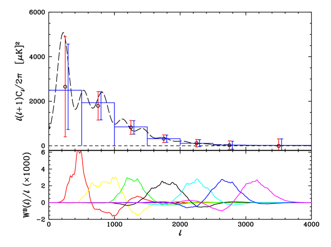
Figure 2: Results of the gridded method plus quadratic relaxation for 387 mock CBI 08h deep-field datasets (upper panel), with each mock observation drawn from an independent realization of the sky given the model power spectrum (shown as the dashed curve) and the instrumental noise with the appropriate rms. The points (black circles) are placed at the band centers, at the mean of the reconstructed bandpowers with the (red) errorbars given by the scatter among the realizations. The (blue) errorbars to the right of the points show the average of the inverse Fisher matrix diagonals. The histograms show the width of each band and the level expected by integrating the model $\cal{C}_{\ell}$ over the window functions $W^{B}_{\ell}$ which are shown in the lower panel. The mean of the realizations converges to the expected value within the Poisson uncertainty, taking into account the correlations between adjacent bands.

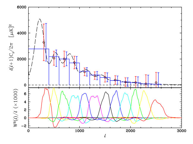
Figure 3: Upper panel shows the results of the gridded method plus quadratic relaxation for 117 mock CBI ($7\times 6$ field) mosaic datasets with a CDM-based power spectrum (the dashed curve). As in Figure 2, the points (black circles) are centered in each bin in $\ell$ with (red) errorbars giving rms scatter of about the mean for the bandpowers from the processed realizations, with the (blue) error bar from average inverse Fisher diagonals to the right of the points. The window functions are plotted in the lower panel.

where ${\cal C}^{({\rm flat})}_{B_{f}}$ are bandpowers calculated using flat filters ($W^{B_{f}}_{\ell}=1$). We find that a fine band width $\Delta\ell_{B_{f}}\sim 20$ is sufficient to adequately sample the window functions and ensure normality and orthogonality to within $0.5\%$ with respect to integration over the bands (e.g. eq.[87]). Example window functions calculated in this manner for mock deep fields and mosaics are shown in the lower panels of Figure 2 and Figure 3 respectively.

7.3 Component Bandpowers

A further complication at the parameter end of the process is that the likelihood of the bandpowers cannot be assumed to be a Gaussian. This is especially so in cases where the error in the bandpowers is sample or cosmic variance limited. Assuming the bandpowers to be Gaussian distributed can lead to the well known problem of cosmic bias where the likelihood of low power models can be overestimated and conversely that of high power models can be underestimated. Bond, Jaffe, & Knox (2000) have shown how one can avoid this problem while still retaining Gaussianity in the $\chi^{2}$ analysis by treating certain functions of the bandpowers as Gaussian distributed. Very good fits to the non-Gaussian distribution of the bandpowers can be obtained by use of the offset log-normal and equal variance approximations to the likelihood.

Both approximations use offsets $x_{B}$ in the bandpowers which describe the contributions to the error in the bandpowers due to components other than the CMB. For the range of scales probed by instruments such as CBI these components will include the foregrounds such as point sources in addition to the usual noise ‘on the sky’ offset $x^{\rm N}_{B}\sim\sum_{\ell}\chi_{B\ell}\,x_{\ell}$, where $x_{\ell}$ is the offset due to the noise contribution to the error such that the quantity $Z_{\ell}=\ln({\cal C}_{\ell}+x_{\ell})$ has a normal distribution Bond, Jaffe, & Knox (2000). For accurate parameter fits we therefore require estimates of bandpowers for all the components making up the total covariance ${\bf C}$. An approximation for these can be obtained by modifying the minimum variance estimator for the bandpowers $q_{B}$ at the maximum likelihood

$$q_{B}^{\rm X}={1\over 2}\,\sum_{B^{\prime}}\left[F_{BB^{\prime}}\right]^{-1}\,{\rm Tr}\left[({\bf C}^{-1}\,{\bf C}^{\rm S}_{B^{\prime}}\,{\bf C}^{-1})\,{\bf C}^{\rm X}\right]$$ (90)

where we have substituted ${\bf C}^{\rm X}$ in equation (77) for the observed measure for the signal covariance $({\bf d}\,{\bf d}^{\rm t}-{\bf C}^{\rm N})$. We then set ${\bf C}^{\rm X}$ to the noise ${\bf C}^{\rm N}$, foreground source ${q}_{\rm src}\,{\bf C}^{\rm src}$ or Gaussian residual foreground ${q}_{\rm res}\,{\bf C}^{\rm res}$ covariance components as desired (or use the maximum likelihood values $\hat{q}_{\rm src}$ and $\hat{q}_{\rm res}$ if these are included as parameters in the solution rather than being fixed). Examples of these are shown in Paper II and Paper III for the deep field data and mosaic data respectively. The offset to the log-normal is then obtained by summing the $q_{B}^{\rm X}$ over the components, $x_{B}\approx q_{B}^{\rm N}+q_{B}^{\rm src}+q_{B}^{\rm res}$ (e.g. Bond & Crittenden 2001). This formalism is used in Paper V to approximate the shapes of the likelihood functions in order to derive limits on the cosmological parameters.

8 Imaging from the Gridded Estimators

Although not the primary goal of this method, an image can be constructed by Fourier transforming back to the sky plane using equation (1). If the estimators $\Delta_{i}$ are constructed on a regular lattice in ${\bf u}_{i}$ with spacing $d_{u}$ and uv extent $L\,d_{u}$, then the resulting image will have an extent on the sky given by the inverse of the spacing $d_{u}^{-1}$ and a resolution given by $d_{u}^{-1}/L$. In the continuum limit (see Appendix A), we can define an estimator $\hat{T}(\mbox{\boldmath$x$})$ for the temperature field ${T}(\mbox{\boldmath$x$})$

$$\hat{T}(\mbox{\boldmath$x$})=\int d^{2}\mbox{\boldmath$u$}\,\Delta(\mbox{\boldmath$u$})\,e^{2\pi i\mbox{\boldmath$\scriptstyle u$}\cdot\mbox{\boldmath$\scriptstyle x$}}$$ (91)

where $\Delta(\mbox{\boldmath$u$})$ is the continuous functional form (e.g. eq[A2]) for the estimators, with $\Delta_{i}=\Delta(\mbox{\boldmath$u$}_{i})$. In practice the lattice of estimators $\Delta_{i}$ is embedded in a wider grid padded with zero in the unsampled cells, and an FFT is carried out.

For our standard gridding normalization $z_{i}=z^{(1)}_{i}$ given in equation (A21), the units of $\Delta$ will be flux density units (Jy) and thus its inverse Fourier transform will produce a map in units of Jy/beam, where the beam area is given by the point-spread-function (PSF) of the image. For a single field, the PSF is just the image generated using equation (91) using estimators $\Delta^{\rm PSF}_{i}$ computed by introducing unit “visibilities” into equation (21)

$$\Delta^{\rm PSF}_{i}=\sum_{k}\big{\{}Q_{ik}+\overline{Q}_{ik}\big{\}}.$$ (92)

The situation for the mosaics is somewhat more complicated, as the mosaic offsets must be taken into account in constructing equivalent visibilities for point sources

$$\Delta^{\rm PSF}_{i}(\hat{\mbox{\boldmath$x$}}) = \sum_{k}\big{\{}Q_{ik}\,V^{\rm PSF}_{k}(\hat{\mbox{\boldmath$x$}})+\overline{Q}_{ik}\,V^{\ast\rm PSF}_{k}(\hat{\mbox{\boldmath$x$}})\big{\}}$$

$$V^{\rm PSF}_{k}(\hat{\mbox{\boldmath$x$}}) = A_{k}(\hat{\mbox{\boldmath$x$}}-\mbox{\boldmath$x$}_{k})e^{-2\pi i\mbox{\boldmath$\scriptstyle u$}_{k}\cdot(\hat{\mbox{\boldmath$\scriptstyle x$}}-\mbox{\boldmath$\scriptstyle x$}_{k})}$$ (93)

obtained by evaluating equation (11) with no noise and $I(\mbox{\boldmath$x$})=\delta^{2}(\mbox{\boldmath$x$}-\hat{\mbox{\boldmath$x$}})$. In this case one would evaluate the PSF at various positions $\hat{\mbox{\boldmath$x$}}$ in the map.

Because our estimators use the kernel ${\bf Q}$ as given in equation (22) which includes the beam transform $\tilde{A}$, we are effectively multiplying the image on the sky by the primary beam squared — once in the kernel, and once due to the instrument itself (e.g. eq.[12]). Images made directly from the $\Delta$ will therefore be strongly attenuated in the (noisy) outskirts.

As mentioned in Appendix A, the optimal weighting for the imaging of the CMB component is to use the Planck factor in equation (6) to correct for the thermal frequency spectrum (e.g. eq.[A20]), while our standard intensity weighting given in equation (A19) is optimized for a flat non-thermal power-law spectrum with spectral index $\alpha=0$.

We can also filter the gridded estimators in such a way as to enhance or down-weight certain signals or noise. We can do this with optimal or Wiener filtering (e.g. Bond & Crittenden 2001),

$$\mbox{\boldmath$\Delta$}^{\phi}={\bf\Phi}\mbox{\boldmath$\Delta$}$$ (94)

where the choice of the filter ${\bf\Phi}$ depends on the application. For example, the covariances ${\bf C}^{\rm X}$ calculated from equation (32) can be used to construct optimal filters for each component contributing to the observations. For the signal component described by the covariances ${\bf C}^{\rm X}$ we can construct a Wiener filter to be applied to the gridded $uv$ estimators

$$\mbox{\boldmath$\Delta$}^{\rm X}={\bf C}^{\rm X}\,{\bf C}^{-1}\,\mbox{\boldmath$\Delta$}.$$ (95)

The amplitudes for the signal models such as the bandpowers $q_{B}$ or the source amplitudes $q_{\rm src}$ can be set to their Maximum Likelihood values or to fiducial model amplitudes. The Wiener filtered image is then recovered by Fourier transforming.

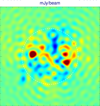
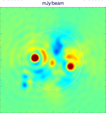
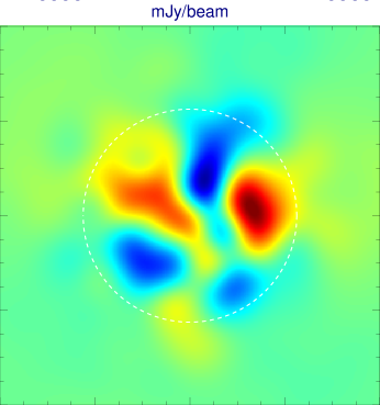
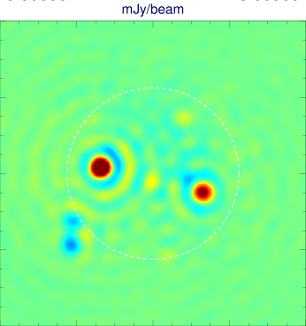
Figure 6: Images reconstructed from the gridded estimators using the formalism of §8. Data is for one of the mock 08h deep-field realizations with sources used in Figure 5. Shown are: Panel (a) upper left — image computed without any filtering; (b) upper right — the image derived by setting ${\bf C}^{\rm X}={\bf C}^{\rm src}+\sum_{B}q_{B}\,{\bf C}^{\rm S}_{B}$ the sum of the signal terms; (c) lower left — the image using ${\bf C}^{\rm X}=\sum_{B}q_{B}\,{\bf C}^{\rm S}_{B}$ for the CMB only; (d) lower right — image for ${\bf C}^{\rm X}={\bf C}^{\rm src}$ to pick out the point sources. The filter clearly dampens the noise, and separates the CMB and source components. The residuals from several bright sources dominate the signal in all but the CMB-filtered image (the brightness scale in that image is enhanced). The white dashed circle shows the $45\farcm 2$ FWHM of the CBI at 31 GHz. The attenuation of the signal brightness due to the square of the primary beam is clearly seen.

Examples of images created using this method are described in the next section, and shown in Figure 6. Wiener-filtered images are also used in Paper VI to explore the possibility of detection of the Sunyaev-Zeldovich effect in the data at high $\ell$.

9 Implementing the Method

The algorithm described above was coded as a scalar Fortran (f77 compatible) program designated cbigridr, with a parallelized Fortran 90 version using OpenMP directives also available for use on multiprocessor machines. In addition, the BJK likelihood relaxation was coded in a second parallelized Fortran 90 program called mlikely using parallel versions of LAPACK matrix algebra routines (e.g. §7). Together, these two programs make up the CBI analysis pipeline. This pipeline has undergone numerous tests and development since its inception in April 2001, and has been used to produce the power spectra and to provide the bandpowers as input to the cosmological parameter analysis given in the companion papers. We now give a brief description of our implementation.

In order to carry out the numerical integrations, a fine-grain rectangular lattice in uv-space was used. The fine-grain grid size $\Delta u_{\rm fine}$ (in units of wavelength) was chosen to adequately sample the phase turns in the uv plane due to the mosaic size and differencing; for a standard $7\times 6$ CBI mosaic with $20^{\prime}$ spacing, the maximum field separation along the grid direction is $x_{\rm max}=2^{\circ}$, which gives oscillations in the uv plane with wavelength of $x_{\rm max}^{-1}=28.65$, giving $\Delta u_{\rm fine}\leq 14.3$ for two samples per cycle. To evaluate the projection operators $R_{i}(\mbox{\boldmath$v$})$ (e.g. eq.[23]), we store a small fine-grain lattice around each $\mbox{\boldmath$u$}_{i}$. The maximum radius in uv space needed for the support of ${\bf R}$ is $r_{u}=2D/\lambda_{\rm min}$. For CBI $D=90$ cm, and $\lambda_{\rm min}=0.844$ cm at $35.5$ GHz, we get $r_{u}=213.1$. A grid of size $53\times 53$ cells with $\Delta u_{\rm fine}=8.526$ will fit both the sampling and radius requirements.

The estimators are evaluated on a coarse-grain lattice of $\mbox{\boldmath$u$}_{i}$, with a spacing of $\Delta u_{\rm coarse}$. The fine-grain lattices on which we accumulate the $R_{i}(\mbox{\boldmath$v$})$ will be cross-correlated to form the covariance elements ${\bf M}_{B}$ and $\overline{\bf M}_{B}$ (e.g. eq.[37]), it is desirable to have the coarse grid size locked to integer multiples of the fine-grid cells. This coarse grid does not have to sample the highest mosaic frequencies, but only the effective width of ${\bf R}$. We find that for single CBI fields, $\Delta u_{\rm coarse}=3\,\Delta u_{\rm fine}$ is adequate. For CBI mosaics, a hybrid lattice with $\Delta u_{\rm coarse}=\Delta u_{\rm fine}$ in the inner part ($\ell<800$) and $\Delta u_{\rm coarse}=2\,\Delta u_{\rm fine}$ in the outer part was found to work well.

As stated in §2, the choice of sign of the exponential of the Fourier transform in equation (1) is a convention. This choice varies throughout the literature on the subject, but in practice depends upon the way the baseline vectors are defined in the data and how the correlation products are made (e.g. which antenna gets the quadrature phase shift). We note that in coding our algorithm to conform to the imaging standards of the AIPS, and DIFMAP (Shepherd, 1997) packages using the CBI data, we had to use the opposite sign convention from the one presented in equation (1).

To process a dataset, a spectral weighting $f(\nu)$ and shape function $C^{\rm shape}_{\ell}$ are chosen. The visibilities $V_{k}$ are looped over, and any source subtraction (§6.3) is applied. For each estimator $i$ that $V_{k}$ contributes to either directly or as a conjugate, its contribution to the fine-grain lattice $q$ for $R_{i}(\mbox{\boldmath$v$}_{q})$ is accumulated, e.g.

$$R_{i}(\mbox{\boldmath$v$}_{q})=\sum_{k}\{Q_{ik}\,P_{k}(\mbox{\boldmath$v$}_{q})+\overline{Q}_{ik}\,\overline{P}_{k}(\mbox{\boldmath$v$}_{q})\}\hskip 56.9055pt\mbox{\boldmath$v$}_{q}=\mbox{\boldmath$u$}_{i}+\Delta u_{\rm fine}\,\hat{\mbox{\boldmath$v$}}_{q}$$ (96)

where $\hat{\mbox{\boldmath$v$}}_{q}$ is a $53\times 53$ unit (fine-grain) lattice. This means that for $n_{\rm est}$ estimators, the storage required for ${\bf R}$ is only $2809\times n_{\rm est}$ double-precision complex numbers. If the data were differenced (as for CBI data), then $P^{\rm sw}_{k}(\mbox{\boldmath$v$})$ from equation (70) is used. The contributions to the noise covariance elements ${\bf M}^{\rm N}$ and $\overline{\bf M}^{\rm N}$ (eq.[35]), and the $\mbox{\boldmath$\Delta$}^{\rm src}_{c}$ (eq.[54]) are also accumulated at this time. Finally, this visibility’s contributions are added to estimator $\Delta_{i}$ and normalization $z_{i}$.

The storage for ${\bf R}$, ${\bf M}^{\rm N}$, and $\overline{\bf M}^{\rm N}$ dominate the memory requirements. For example, the CBI mosaics use around $n_{\rm est}=2500$ estimators, and thus storage for $53\times 53\times 2500\approx 7\times 10^{6}$ double-precision complex numbers is needed. A single packed $n^{2}_{\rm est}\approx 6\times 10^{6}$ array is needed to hold ${\bf M}^{\rm N}$ and $\overline{\bf M}^{\rm N}$. The ${\bf C}^{\rm X}$ matrices are calculated in place and written out row by row, and thus need not be stored. There are no instances where matrices of dimension $N_{\rm vis}^{2}$ are stored; the storage for a matrix of this size would be prohibitive as our largest CBI mosaics have $N_{\rm vis}>2\times 10^{5}$.

When all the visibilities have been processed, the estimators are normalized by $z_{i}$, split into real and imaginary parts, and written out to disk. The covariance matrices $C^{\rm N}_{ij}$, $C^{\rm S}_{Bij}$, and any $C^{\rm src}_{ij}$ are constructed by looping over pairs of rows corresponding to the real and imaginary parts of each estimator, e.g. rows $i$ and $i+N_{\rm est}$ for estimator $i$. For each $j\leq i$, the stored $R_{i}$ and $R_{j}$ are cross-correlated along with the shape function ${\cal C}(|\mbox{\boldmath$v$}|)$ to form the bandpower covariance elements $M_{Bij}$ and $\overline{M}_{Bij}$ of equation (37), combined to make $C^{\rm S}_{Bij}$ using equation (32), and stored. The relevant columns of these rows of $C^{\rm N}_{ij}$ are formed from the stored $M^{\rm N}_{ij}$ and $\overline{M}^{\rm N}_{ij}$. At this point, for each ${\bf C}^{\rm src}$ desired (there may be more than one, in the CBI analysis we use 3), the relevant $\Delta^{\rm src}_{c}$ are combined using equation (55) to form $M^{\rm src}_{ij}$ and $\overline{M}^{\rm N}_{ij}$, which in turn are used to make $C^{\rm src}_{ij}$. After all columns for these rows of the covariance matrices are computed, they are written to disk, and this process is repeated for the pair of rows corresponding to the next estimator $i$. When all rows are complete, the output file is complete. Note that different binnings of the ${\bf C}^{\rm S}_{B}$ can be run without regridding using the original ${\bf R}$, saving significant time.

If a residual foreground covariance matrix ${\bf C}^{\rm res}$ is desired, the procedure outlined above is repeated in its entirety using the description in §6.4. The spectrum and shape appropriate for the source population or foreground emission is used during the gridding and covariance matrix construction. Other than these factors, the same gridding as in the CMB and noise estimators must be used.

The output files from cbigridr are then used as input to mlikely. These can be for single fields or mosaics, or for combinations of independent fields or mosaics (§7.1). At this point, the pre-factors $q_{\rm src}$ and $q_{\rm res}$ for any ${\bf C}^{\rm src}$ and ${\bf C}^{\rm res}$ covariance matrices are chosen and fixed. Relaxation to the likelihood maximum is carried out as described in §7, and the resulting bandpowers $\{q_{B}\}$ and inverse Fisher matrix elements $[F^{-1}]_{BB^{\prime}}$ are written out. If desired, the bandpower window functions $W^{B}_{B_{f}}$ (§7.2) can be computed if cbigridr was run to produce narrow-bin ${\bf C}^{\rm S}_{B_{f}}$. The component bandpowers $q_{B}^{\rm N}$, $q_{B}^{\rm src}$ and $q_{B}^{\rm res}$ (§7.3) can also be computed at this time.

Finally, filtered images using the formalism of §8 can be computed from the estimators, the ${\bf C}$ (at maximum likelihood), and the component covariance matrices. Results from this are shown below and in Paper VI.

The timing for cbigridr depends upon the degree of parallelization as well as the processor speed on a given machine, and the number of visibilities gridded, number of foreground sources, and number of bins $B$ for the bandpowers. As an example, the processing of the 14-h mosaic field of Paper III (the largest of the datasets) involved gridding 228819 visibilities from 65 separate nights of data in 41 fields to 2352 complex estimators. A total of 916 sources were gridded into three source covariance matrices. A total of 7 different binnings for ${\bf C}^{\rm S}_{B}$ were run at this time from the same gridding. The execution time using the parallel version of cbigridr was $2^{\rm h}\,40^{\rm m}$ running on 22 processors on a 32-processor Alpha GS320 workstation at the Canadian Institute for Theoretical Astrophysics. It then took $3^{\rm h}\,22^{\rm m}$ on the same computer for mlikely to process 4704 double-precision real estimators in 16 ${\bf C}^{\rm S}_{B}$ bands, with 3 ${\bf C}^{\rm src}$ matrices, one ${\bf C}^{\rm res}$ and one ${\bf C}^{\rm N}$. This included the time needed to calculate the component bandpowers ${\bf C}^{\rm X}_{B}$, but not the window functions. The speed of this fast gridded method has allowed us to carry out numerous tests on both real and simulated dataset, which would not have been possible carrying out maximum likelihood (e.g. using even the optimized mlikely) on the 200000-plus visibilities.

9.1 Method Performance Tests Using Mock CBI Data

The performance of the method was assessed by applying it to mock CBI datasets. Simulated CBI datasets were obtained by replacing the actual visibilities from the data files containing real CBI observations of the various fields used in Paper II and Paper III with the response expected for a realization of the CMB sky drawn from a representative power spectrum, plus uncorrelated Gaussian instrumental noise with the same variance as given by the scatter in the actual CBI visibilities. The differencing of the lead and trail fields used in CBI observations was included (e.g. §6.6). This mock dataset had the same uv distribution as the real data, and gives an accurate demonstration of expected sensitivity levels and the effect of cosmic variance. The power spectrum chosen for these simulations was for a model that fit the COBE and BOOMERANG data (Netterfield et al., 2001).

Figure 2 shows the power spectrum estimation derived following the procedure detailed above. The mock datasets were drawn as realizations for the 08h CBI deep field from Paper II. The binning of the signal covariance matrix ${\bf C}^{\rm S}_{B}$ was chosen to be uniform in $\ell$ with bin width $\Delta\ell=500$. Because a single realization of the sky drawn from the model power spectrum will have individual mode powers that deviate from mean given by the power spectrum due to this intrinsic so-called “cosmic variance” plus the effect of the thermal instrumental noise, we analyze 387 realizations each taken from a different realization of the sky and a different set of instrumental noise deviates. The mean $q_{B}$ for each band $B$ converge to $\langle C_{B}\rangle$, which is obtained by integrating the model $\cal{C}_{\ell}$ over the window functions $W^{B}_{\ell}$ (e.g. eq.[89]), within the sample uncertainty for the realizations. Furthermore, the standard deviation of the $q_{B}$ from the mean for each band agrees with the value obtained from the diagonals of the inverse of the Fisher matrix.

The choice of the $\ell$ bin size is driven by the trade off between the desired narrow bands for localizing features in the power spectrum and the correlations between bins introduced by the transform of the primary beam. There is an anti-correlation between adjacent bands seen in $[F^{-1}]_{BB^{\prime}}$ at the level of $-13$% to $-23$% for $\Delta\ell=500$ with a single field. We have found that correlations up to about $-25$% give plots of the $q_{B}$ that are more visually appealing than those made with narrower band and higher correlation levels due to the increasing scatter in the bandpowers about the mean values. Bins of this size do not achieve the best possible $\ell$-resolution, and thus our cosmological parameter runs use finer-binned bands since the correlations are taken into account in the analyses.

The band window functions $W^{B}_{\ell}$ are shown in the lower panel of Figure 2, and were computed using narrow binnings $W^{B}_{B_{f}}$ (e.g. eq.[88]) with $\Delta\ell=20$. The small-scale structures seen in the window functions, particularly visible around the peaks, are due to the differencing which introduces oscillations (see §6.6). As shown in equation (87), a window function $W^{B}_{\ell}$ is normalized to sum to unity within the given band $B$, and to sum to zero in the other bands, and thus there must be compensatory positive and negative “sidelobes” of the window function outside the band.

Figure 3 shows the power spectrum derived for a simulated mosaic of $7\times 6$ fields separated by $20^{\prime}$ using the actual CBI 20h mosaics fields from Paper III as a template. This mosaic field was chosen as it had incomplete mosaic coverage, and thus would be the most difficult test for the method. The binning for ${\bf C}^{\rm S}_{B}$ shown used $\Delta\ell=200$, which gave adjacent band anti-correlations of $-13\%$ to $-18\%$ in the $F_{BB^{\prime}}$. Again the mean of the 117 realizations converges to the value expected within the error bars, showing that there is no bias introduced by the method, even in the presence of substantial holes in the mosaic (see Paper III for the mosaic weight map). Furthermore, the rms scatter in the realizations converges to the mean of the inverse Fisher error bars, as in the single-field case. As in the previous figures, the bandpower window functions are shown in the lower panels.

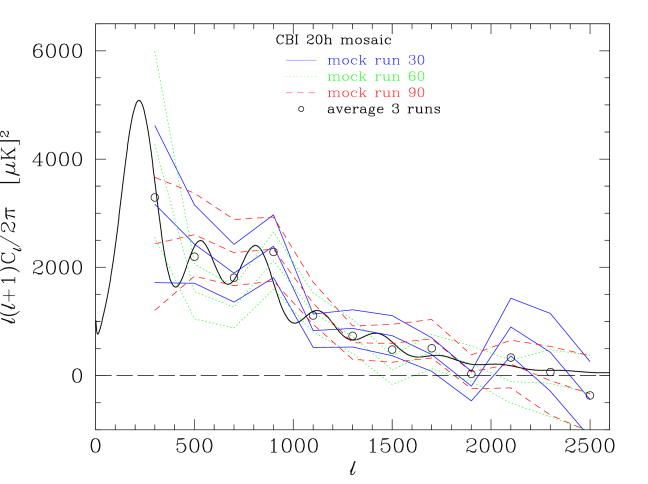
Figure 4: Three randomly selected realizations from the mosaic field simulations shown in Figure 3 are shown plotted against the model power spectrum (solid black curve). The three lines for the bandpowers reconstructed from the three realizations correspond to the bandpowers (central lines) and the $\pm 1\,\sigma$ excursions using the inverse Fisher errorbars. The scatter in bandpowers between realizations is within the expected range. Also shown is the unweighted scalar average of the bandpowers for the 3 realizations, which is an approximation to a true joint likelihood solution. The average is a better fit to the model, as is expected.

In Figure 4 are shown three randomly chosen realizations from the ensemble, plotted along with the input power spectrum. This shows the level of field-to-field variations that we might expect to see in CBI data. There are noticeable deviations from the expected bandpowers in individual realizations, particularly at low $\ell$ where cosmic variance and the highly-correlated bins conspire to increase the scatter. These differences are within the expected scatter when bin-bin correlations and limited sample size is taken into account, but care must be exercised in interpreting single field power spectra. In particular, the acoustic peak structures are obscured by the sample variations. However, the average bandpowers for the 3 runs (shown in Figure 4 as open black circles) are better representations of the underlying power spectrum. Although this is not a proper “joint” maximum likelihood solution (e.g. §7.1) as is done for the real CBI mosaic fields, the improvement seen using the 3-field average leads us to expect that the combination of even 3 mosaic fields damps the single field variations sufficiently to begin to see the oscillatory features in the CMB power spectrum. While we do not show the equivalent plots of the deep fields from Figure 2, the same behavior is seen (with even larger field-to-field fluctuations in the relatively unconstrained first bin, though still consistent with the error bars).

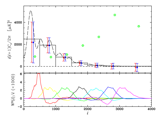
Figure 5: Results using mock deep-field datasets including foreground point sources based on the actual list used in the CBI data are shown (upper panel) along with the window functions (lower panel). The input power spectrum and expected bandpowers are as in Figure 2. The (green) stars show the average for 200 realizations where no source subtraction or projection was done, with the powers divided by a factor of 2 to fit on the plot. The expected increase with $\ell^{2}$ is seen, along with a falloff in the last bin due to the source frequency spectrum. The points with errorbars at the center of each bin (red triangles) were computed from 200 realizations processed with subtraction of the mean flux density from the visibilities and construction of ${\bf C}^{\rm src}$ using the uncertainties, while the points with errorbars to the right of these (blue squares) are from 200 realizations where no source subtraction was done, but we built ${\bf C}^{\rm src}$ using the full (unperturbed) flux densities which projects out the sources with only a slight increase in noise. Despite the large power from sources at high $\ell$, our method successfully removes the foreground power from the spectrum with no sign of bias.

The effect of adding point sources to the mock fields, and then attempting power spectrum extraction, is shown in Figure 5. A set of 200 realizations were made in the same manner as in the runs in Figure 2, but the list of point source positions, flux densities and uncertainties, and spectral indices from lower frequency used in the analysis in Paper II (the “NVSS” sources) was used to add mock sources to the data. The flux density of the sources actually added to the data were perturbed using the stated uncertainties as 1-$\sigma$ standard deviations. The errors used were 33% of the flux density except for a few of the brighter sources which were put in with 100% uncertainties. We then used the methodology described in §6.3 to compute the constraint matrices. The first method of correction used was to subtract the (unperturbed) flux densities from the visibilities, and build the ${\bf C}^{\rm src}$ from $\mbox{\boldmath$\Delta$}^{\rm src}$ built using the uncertainties (shown as the red triangles). In addition, we also did no subtraction, but built ${\bf C}^{\rm src}$ from $\mbox{\boldmath$\Delta$}^{\rm src}$ using the full (unperturbed) flux densities (shown as the blue squares). This is equivalent to assuming a 100% error on the source flux densities, and thus canceling the average source power in those modes. In both cases the factor $q_{\rm src}=1$ was used. The simulations show that both methods are effective, with no discernible bias in the reconstructed CMB bandpowers.

Finally, the production of images using the gridded estimators described in §8 is demonstrated in Figure 6. The series of plots show the effect of Wiener filtering using the noise and various signal components on an image derived from one of the mock 08h CBI deep field realizations with sources from the ensemble shown in Figure 5. The Planck factor weighting of equation (A20) was used during gridding to optimize for the thermal CMB spectrum, though in practice this makes little difference due to the restricted frequency range of the CBI. The estimators for this realization were computed by subtracting the mean values of the source flux densities and putting the standard deviations into ${\bf C}^{\rm src}$ with $q_{\rm src}=1$ (the red triangles in Figure 5). The filtering down-weights the high spatial frequency noise seen in the unfiltered image, and effectively separates the CMB and source components as shown by comparing panels (c) and (d) to the total signal in panel (b). The signal in this realization is dominated by the residuals from two bright point sources that had 100% uncertainties put in for their flux densities and thus escaped subtraction. The effectiveness of ${\bf C}^{\rm src}$ in picking out the sources in the image plane underlines its utility as a constraint matrix in the power spectrum estimation.

10 Conclusions

We have outlined a maximum likelihood approach to determining the power spectrum of fluctuations from interferometric CMB data. This fast gridded method is able to handle the large amounts of data produced in large mosaics such as those observed by the CBI. Software encoding this algorithm was written, and tested using mock CBI data drawn from a realistic power spectrum. The results of the code were shown to converge as expected to the input power spectrum with no discernible bias. For small datasets, this code was also tested against independently written software that worked directly on the visibilities. In addition, the pipeline was run with gridding turned off as described in §6, again for small test data sets. No bias or significant loss in sensitivity was seen in these comparisons.

This software pipeline was used to analyze the actual CBI data, producing the power spectra presented for the deep fields and mosaics in Paper II and Paper III respectively. The output of the pipeline also was used as the input for the cosmological parameter analysis in Paper V and the investigation of the Sunyaev-Zeldovich Effect in Paper VI.

This method is of interest for carrying out power spectrum estimation for interferometer experiments that produce a large number of visibilities but with a significantly smaller number of independent samples of the Fourier plane (such as close-packed arrays such as VSA or DASI). The CBI pipeline analysis is carried out in two parts, the gridding and covariance matrix construction from input uv-FITS files in cbigridr and the maximum likelihood estimation of bandpowers using quadratic relaxation in mlikely. The software for the pipeline is available by contacting the authors.

We close by noting that our formalism can be extended to deal with polarization data. In the case of CMB polarization, there are as many as six different signal covariance matrices of interest in each band, with estimators (or visibilities) for parallel-hand and cross-hand polarization products, and thus development of a fast method such as this is critical. In September 2001 polarization capable versions of cbigridr and mlikely were written and tested. We describe the method, the polarization pipeline, and results in the upcoming paper (Myers et al. 2002, in preparation).

Appendix A Form of the Linear Estimator

Suppose we were to construct a simple linear “dirty” mosaic on the sky obtained by a linear combination of the dirty (not deconvolved) images of the individual fields (e.g. Cornwell, Holdaway, & Uson 1993). In the uv plane, this reduces to summing (integrating) up the visibilities from each mosaic “tile” with some weighting function, e.g.

$$\Delta_{i}=\sum_{k}Q_{ik}\,V_{k}$$ (A1)

where for the time being we ignore the contribution from the complex conjugates of the visibilities (see below). For illustrative purposes, let us consider only a single frequency channel and write the estimator as a function $\Delta(\mbox{\boldmath$u$})$, where $\Delta_{i}=\Delta(\mbox{\boldmath$u$}_{i})$, which in the absence of instrumental noise is given by

$$\Delta(\mbox{\boldmath$u$})=\int d^{2}\mbox{\boldmath$v$}\,\int d^{2}\mbox{\boldmath$x$}\,{\cal F}(\mbox{\boldmath$x$},\mbox{\boldmath$v$})\,{\cal Q}(\mbox{\boldmath$u$},\mbox{\boldmath$x$},\mbox{\boldmath$v$})\,\langle V(\mbox{\boldmath$x$},\mbox{\boldmath$v$})\rangle$$ (A2)

with kernel ${\cal Q}$, sky and aperture plane sampling given by ${\cal F}$, and where

$$V(\mbox{\boldmath$x$},\mbox{\boldmath$v$})=\int d^{2}\mbox{\boldmath$v$}^{\prime}\,\tilde{I}(\mbox{\boldmath$v$}^{\prime})\,\tilde{A}(\mbox{\boldmath$v$}-\mbox{\boldmath$v$}^{\prime})\,e^{2\pi i\mbox{\boldmath$\scriptstyle v$}^{\prime}\cdot\mbox{\boldmath$\scriptstyle x$}}$$ (A3)

is the visibility at pointing position $x$ and uv locus $v$ from equation (11). In practice, the sampling function is just a series of delta functions

$${\cal F}(\mbox{\boldmath$x$},\mbox{\boldmath$v$})=\sum_{k}\omega_{k}\,\delta^{2}(\mbox{\boldmath$x$}-\mbox{\boldmath$x$}_{k})\,\delta^{2}(\mbox{\boldmath$v$}-\mbox{\boldmath$u$}_{k})$$ (A4)

over the measured visibilities $k=1,\ldots,N_{\rm vis}$ each with weight $\omega_{k}$.

As an ansatz, we let the mosaicing kernel have the form

$${\cal Q}(\mbox{\boldmath$u$},\mbox{\boldmath$x$},\mbox{\boldmath$v$})=Q(\mbox{\boldmath$v$}-\mbox{\boldmath$u$})\,e^{-2\pi i\mbox{\boldmath$\scriptstyle u$}\cdot\mbox{\boldmath$\scriptstyle x$}}$$ (A5)

where $Q$ is the interpolating kernel. Furthermore, let us assume that the uv-plane coverage is the same for all mosaic pointings, and thus ${\cal F}(\mbox{\boldmath$x$},\mbox{\boldmath$v$})$ is separable

$${\cal F}(\mbox{\boldmath$x$},\mbox{\boldmath$v$})\equiv F(\mbox{\boldmath$v$})\,G(\mbox{\boldmath$x$})$$ (A6)

where $F(\mbox{\boldmath$v$})$ and $G(\mbox{\boldmath$x$})$ are the sampling and weighting in the two domains. Combining these and rearranging terms, we get

$$\Delta(\mbox{\boldmath$u$}) = \int d^{2}\mbox{\boldmath$v$}^{\prime}\,\tilde{I}(\mbox{\boldmath$v$}^{\prime})\,\int d^{2}\mbox{\boldmath$v$}\,F(\mbox{\boldmath$v$})\,Q(\mbox{\boldmath$v$}-\mbox{\boldmath$u$})\,\tilde{A}(\mbox{\boldmath$v$}-\mbox{\boldmath$v$}^{\prime})\,\int d^{2}\mbox{\boldmath$x$}\,G(\mbox{\boldmath$x$})\,e^{-2\pi i(\mbox{\boldmath$\scriptstyle u$}-\mbox{\boldmath$\scriptstyle v$}^{\prime})\cdot\mbox{\boldmath$\scriptstyle x$}}$$ (A7)

$$= \int d^{2}\mbox{\boldmath$v$}^{\prime}\,\tilde{I}(\mbox{\boldmath$v$}^{\prime})\,\tilde{G}(\mbox{\boldmath$u$}-\mbox{\boldmath$v$}^{\prime})\,\int d^{2}\mbox{\boldmath$v$}\,F(\mbox{\boldmath$v$})\,Q(\mbox{\boldmath$v$}-\mbox{\boldmath$u$})\,\tilde{A}(\mbox{\boldmath$v$}-\mbox{\boldmath$v$}^{\prime})$$ (A8)

where in equation (A8) we used the fact that the final right-hand side integral in equation (A7) is the Fourier transform $\tilde{G}$ of the mosaic function ${G}$.

For an infinite continuous mosaic, $\tilde{G}(\mbox{\boldmath$v$}^{\prime}-\mbox{\boldmath$u$})=\delta^{2}(\mbox{\boldmath$v$}^{\prime}-\mbox{\boldmath$u$})$ and thus

$$\Delta(\mbox{\boldmath$u$})=\tilde{I}(\mbox{\boldmath$u$})\,\int d^{2}\mbox{\boldmath$v$}\,F(\mbox{\boldmath$v$})\,Q(\mbox{\boldmath$v$}-\mbox{\boldmath$u$})\,\tilde{A}(\mbox{\boldmath$v$}-\mbox{\boldmath$u$}).$$ (A9)

If we wish to recover $\Delta(\mbox{\boldmath$u$})=\tilde{I}(\mbox{\boldmath$u$})$ in this limit, then

$$Q(\mbox{\boldmath$v$}-\mbox{\boldmath$u$})={1\over z(\mbox{\boldmath$u$})}\,\tilde{A}^{\ast}(\mbox{\boldmath$v$}-\mbox{\boldmath$u$})$$ (A10)

with normalization

$$z(\mbox{\boldmath$u$})=\int d^{2}\mbox{\boldmath$v$}\,F(\mbox{\boldmath$v$})\,\tilde{A}^{2}(\mbox{\boldmath$v$}-\mbox{\boldmath$u$})$$ (A11)

will fulfill our requirements. We have chosen $\tilde{A}^{\ast}(\mbox{\boldmath$v$}-\mbox{\boldmath$u$})$ as the uv kernel as it reproduces the least-squares estimate of the sky brightness in the linear mosaic (Cornwell, Holdaway, & Uson, 1993). Then, equation (A8) becomes

$$\Delta(\mbox{\boldmath$u$})={1\over z(\mbox{\boldmath$u$})}\,\int d^{2}\mbox{\boldmath$v$}^{\prime}\,\tilde{I}(\mbox{\boldmath$v$}^{\prime})\,\tilde{G}(\mbox{\boldmath$u$}-\mbox{\boldmath$v$}^{\prime})\,\int d^{2}\mbox{\boldmath$v$}\,F(\mbox{\boldmath$v$})\,\tilde{A}^{\ast}(\mbox{\boldmath$v$}-\mbox{\boldmath$u$})\,\tilde{A}(\mbox{\boldmath$v$}-\mbox{\boldmath$v$}^{\prime})$$ (A12)

which has a width controlled by the narrower of the width of $\tilde{A}^{2}$ or the width of $\tilde{G}$. Thus, by widening the mosaic $G({\bf x})$ to a larger area than the beam $A$, we will fill in the desired information inside the $\tilde{A}$ smeared patches in the uv-plane. Thus, a properly sampled $M^{2}$ mosaic will fill in a $M^{2}$ sub-grid within each uv cell you would have normally had for a single pointing, and thus an $M^{2}$ mosaic consisting of $N^{2}$ “images” each is equivalent to a uv super-grid of size $(M\times N)^{2}$ (e.g. Ekers & Rots 1979).

Note that for a non-continuous mosaic, there will be “aliases” in the uv plane separated by the inverse of the mosaic spacing in the sky (Cornwell, 1988). Ideally, we would like the separation between aliased copies to be larger than the extent of the beam transform, which is satisfied for $\Delta x\leq\lambda/2D$ which for $D=90$ cm corresponds to $21\farcm 6$ at $26.5$ GHz and only $16\farcm 1$ at $35.5$ GHz, the centers of the extremal CBI bands. The spacing used in the CBI mosaics is a compromise between the aliasing limits over the bands and the desire to have a fewer number of pointings on a convenient grid. We chose to observe with pointing centers separated by $20^{\prime}$, which is sub-optimal above $27.5$ GHz. However, the effect of aliasing is small, with the overlap point $a^{-1}-D\,\lambda^{-1}$ occurring at the $0.61\%$ point of $\tilde{A}$ at 31 GHz, and the $6.5\%$ point for the highest frequency channel at $35.5$ GHz.

We obtain the gridding kernel $Q_{ik}$ of equation (A1) corresponding to equation (A10) by using the discrete sampling in equation (A4)

$$Q_{ik}={\omega_{k}\over z_{i}}\,\tilde{A}_{k}^{\ast}(\mbox{\boldmath$u$}_{k}-\mbox{\boldmath$u$}_{i})\,e^{-2\pi i\mbox{\boldmath$\scriptstyle u$}_{i}\cdot\mbox{\boldmath$\scriptstyle x$}_{k}}$$ (A13)

with visibility weights $\omega_{k}$, and normalization factor $z_{i}$. The discrete form of the normalization derived in equation (A11) is

$$z_{i}=\sum_{k}\omega_{k}\,\tilde{A}_{k}^{2}(\mbox{\boldmath$u$}_{k}-\mbox{\boldmath$u$}_{i}).$$ (A14)

Then,

$$\Delta_{i}={1\over z_{i}}\,\sum_{k}\omega_{k}\,\tilde{A}_{k}^{\ast}(\mbox{\boldmath$u$}_{k}-\mbox{\boldmath$u$}_{i})\,V_{k}\,e^{-2\pi i\mbox{\boldmath$\scriptstyle u$}_{i}\cdot\mbox{\boldmath$\scriptstyle x$}_{k}}$$ (A15)

is the weighted sum of visibilities used for the estimators. Note that because $V(\mbox{\boldmath$u$})=V^{\ast}(-\mbox{\boldmath$u$})$, there are also visibilities $V_{k^{\prime}}$ for which $-\mbox{\boldmath$u$}_{k^{\prime}}$ lies within the support range around $\mbox{\boldmath$u$}_{i}$, i.e. $\big{|}\tilde{A}_{k^{\prime}}^{\ast}(-\mbox{\boldmath$u$}_{k^{\prime}}-\mbox{\boldmath$u$}_{i})\big{|}>0$. Thus, we should add in the complex conjugates $V^{\ast}_{k}$

$$\Delta_{i}={1\over z_{i}}\,\sum_{k}\omega_{k}\,\big{\{}\tilde{A}_{k}^{\ast}(\mbox{\boldmath$u$}_{k}-\mbox{\boldmath$u$}_{i})\,V_{k}+\tilde{A}_{k}^{\ast}(-\mbox{\boldmath$u$}_{k}-\mbox{\boldmath$u$}_{i})\,V^{\ast}_{k}\big{\}}\,e^{-2\pi i\mbox{\boldmath$\scriptstyle u$}_{i}\cdot\mbox{\boldmath$\scriptstyle x$}_{k}}.$$ (A16)

To do this, we construct another kernel $\overline{Q}_{ik}$

$$\overline{Q}_{ik}={\omega_{k}\over z_{i}}\,\tilde{A}_{k}^{\ast}(-\mbox{\boldmath$u$}_{k}-\mbox{\boldmath$u$}_{i})\,e^{-2\pi i\mbox{\boldmath$\scriptstyle u$}_{i}\cdot\mbox{\boldmath$\scriptstyle x$}_{k}}$$ (A17)

which will gather the appropriate $V^{\ast}_{k}$, giving

$$\Delta_{i}=\sum_{k}\big{\{}Q_{ik}\,V_{k}+\overline{Q}_{ik}\,V^{\ast}_{k}\big{\}}$$ (A18)

for the final form of our linear estimator.

For estimated visibility variances $\epsilon^{2}_{k}$, the optimal weighting factor (in the least-squares estimation sense) is given by

$$\omega_{k}={1\over\epsilon^{2}_{k}}$$ (A19)

but may also include factors based on position in the mosaic or frequency channel. For example, up until now we have neglected the frequency dependence of the observed visibilities. If we are reconstructing an intensity field with a uniform flux density spectrum, then no changes need be made. If there is a frequency dependence, such as that for a power-law foreground (e.g. eq.[7]) or the thermal spectrum of the CMB (e.g. eq.[6]), then the visibilities should be scaled and weighted by the appropriate factor $f_{k}$ when gridded in order to properly estimate $\tilde{I}_{0}(\mbox{\boldmath$u$}_{k})$ or $\tilde{T}(\mbox{\boldmath$u$}_{k}$ respectively. For example, for the CMB using equation (6) for the spectrum, we find

$$Q^{\rm T}_{ik} = {f_{\rm T}^{-1}(\nu_{k})\,\omega_{k}\over z_{i}}\,\tilde{A}_{k}^{\ast}(\mbox{\boldmath$u$}_{k}-\mbox{\boldmath$u$}_{i})$$

$$\omega_{k} = {f_{\rm T}^{2}(\nu_{k})\over\epsilon^{2}_{k}}.$$ (A20)

In practice for the CBI, the frequency range of the data is not great enough for the spectral weighting factor to matter, and we therefore use the default weighting given in equation (A19). This will therefore be slightly non-optimal in the signal-to-noise sense (it will not be the minimum-variance estimator) but it will not introduce a bias in the bandpowers.

The choice of the normalization $z_{i}$ is somewhat arbitrary, as it only determines the units of the $\Delta_{i}$ and not the correlation properties. However, this can be important if we wish to use the estimators to make images using the formalism of §8. For instance, the normalization given in equation (A14) has the drawback of diverging in cells where all the $\tilde{A}_{k}^{2}$ are vanishingly small (such as the innermost and outermost supported parts of the uv-plane), and will produce images with heightened noise on short and long spatial wavelengths. It is therefore more convenient to use the alternate normalization

$$z_{i}=\sum_{k}\omega_{k}\,\tilde{A}^{\ast}_{k}(\mbox{\boldmath$u$}_{k}-\mbox{\boldmath$u$}_{i})$$ (A21)

which when inserted into equation (A15) will properly normalize the weighted sums of visibilities. This will then produce images with the desired units of Janskys per beam (see §8). We therefore use equation (A21) for the normalization in our CBI pipeline.

Appendix B Source Counts and the Residual Covariance Matrix

We wish to calculate ${C}^{\rm res}_{\nu}$ (cf. eq.[67]) using equation (66) with $\nu_{k}=\nu_{k^{\prime}}=\nu$. If $p(\alpha|\nu_{0})$ is independent of flux density, then

$${C}^{\rm res}_{\nu}=\int_{-\infty}^{\infty}d\alpha\,p(\alpha|\nu_{0})\,\left({\nu\over\nu_{0}}\right)^{2\alpha}\int_{0}^{S_{\rm max}(\alpha)}dS\,S^{2}\,{dN(S)\over dS}\,$$ (B1)

where we have left in the possibility that the upper flux density cutoff will depend on spectral index (see below) and set the lower flux density cutoff to zero (the results for realistic power-law counts with $\gamma>-2$ are insensitive to the lower cutoff, but one can easily be included). As an example for the calculation of the fluctuation power due to residual sources in the Gaussian limit, consider power-law integral source counts

$$N(>S)=N_{0}\,\left({S\over S_{0}}\right)^{\gamma}\Rightarrow{dN(S)\over dS}=-{\gamma\,N_{0}\over S_{0}}\,\left({S\over S_{0}}\right)^{\gamma-1}$$ (B2)

where $N(>S)$ is the mean number density of sources with flux density greater than $S$ at frequency $\nu_{0}$, and a Gaussian spectral index distribution at frequency $\nu_{0}$

$$p(\alpha|S,\nu_{0})=p(\alpha|\nu_{0})={1\over\sqrt{2\pi\sigma^{2}_{\alpha}}}\,e^{-{(\alpha-\alpha_{0})^{2}\over 2\sigma^{2}_{\alpha}}}.$$ (B3)

First consider the case where there is a fixed flux density upper cutoff $S_{\rm max}$ at the frequency where the number counts are defined. The two parts of equation (67) separate easily, where the source count part of the integral is

$$\int_{0}^{S_{\rm max}}dS\,S^{2}\,{dN(S)\over dS}\,=-{\gamma\over\gamma+2}\,N_{0}\,S^{2}_{0}\,\left({S_{\rm max}\over S_{0}}\right)^{\gamma+2}.$$ (B4)

For the distribution in equation (B3), the integral over $\alpha$ becomes

$$\int_{-\infty}^{\infty}d\alpha\,p(\alpha|\nu_{0})\,\left({\nu\over\nu_{0}}\right)^{2\alpha} = \int_{-\infty}^{\infty}{d\alpha\over\sqrt{2\pi\sigma^{2}_{\alpha}}}\,e^{-{(\alpha-\alpha_{0})\over 2\sigma^{2}_{\alpha}}}\,e^{2\alpha\,\beta}$$ (B5)

$$= e^{-{(\bar{\alpha}^{2}-\alpha^{2}_{0})^{2}\over 2\sigma^{2}_{\alpha}}}\,\int_{-\infty}^{\infty}{d\alpha\over\sqrt{2\pi\sigma^{2}_{\alpha}}}\,e^{-{(\alpha-\bar{\alpha})^{2}\over 2\sigma^{2}_{\alpha}}}$$

$$= e^{2\alpha_{\rm eff}\,\beta}$$

where $\beta=\ln(\nu/\nu_{0})$, and

$$\alpha_{\rm eff} = {\bar{\alpha}^{2}-\alpha^{2}_{0}\over 4\beta\,\sigma^{2}_{\alpha}}=\alpha_{0}+\beta\,\sigma^{2}_{\alpha}$$

$$\bar{\alpha} = \alpha_{0}+2\beta\,\sigma^{2}_{\alpha}$$ (B6)

where $\bar{\alpha}$ is the mean of the extrapolated spectral index distribution which remains a Gaussian, and the effective spectral index $\alpha_{\rm eff}$ for the spectral component is shifted from the mean spectral index of the input distribution $\alpha_{0}$ by the combination of the scatter in the $\alpha$ and the lever arm $\beta$ from the frequency extrapolation. Putting these together, we get

$${C}^{\rm res}_{\nu}=-{\gamma\over\gamma+2}\,N_{0}\,S^{2}_{0}\,\left({S_{\rm max}\over S_{0}}\right)^{\gamma+2}\,e^{2\alpha_{\rm eff}\,\beta}.$$ (B7)

One can also deal with the case where there is an upper flux density cutoff $\hat{S}_{\rm max}$ imposed at a frequency $\hat{\nu}$ other than $\nu_{0}$ where the $N(S)$ distribution is defined. In this case, the flux density cutoff in equation (B1) is

$$S_{\rm max}(\alpha)=\bar{S}_{\rm max}\,e^{(\alpha_{0}-\alpha)\,\hat{\beta}}\hskip 56.9055pt\bar{S}_{\rm max}=\hat{S}_{\rm max}\,e^{-\alpha_{0}\,\hat{\beta}}$$ (B8)

where $\hat{\beta}=\ln(\hat{\nu}/\nu_{0})$, and $\bar{S}_{\rm max}$ is the cutoff $\hat{S}_{\rm max}$ extrapolated to $\nu_{0}$ using $\alpha_{0}$. Then,

$$\int_{0}^{S_{\rm max}(\alpha)}dS\,S^{2}\,{dN(S)\over dS}=-{\gamma\over\gamma+2}\,N_{0}\,S^{2}_{0}\,\left({\bar{S}_{\rm max}\over S_{0}}\right)^{\gamma+2}\,e^{(\alpha_{0}-\alpha)\,\hat{\beta}\,(\gamma+2)}\\$$

and thus

$${C}^{\rm res}_{\nu} = -{\gamma\over\gamma+2}\,N_{0}\,S^{2}_{0}\,\left({\bar{S}_{\rm max}\over S_{0}}\right)^{\gamma+2}\,\int_{-\infty}^{\infty}d\alpha\,p(\alpha|\nu_{0})\,e^{2\alpha\,\beta}\,e^{(\alpha_{0}-\alpha)\,\hat{\beta}\,(\gamma+2)}$$ (B9)

$$= -{\gamma\over\gamma+2}\,N_{0}\,S^{2}_{0}\,\left({\bar{S}_{\rm max}\over S_{0}}\right)^{\gamma+2}\,e^{2\hat{\alpha}_{\rm eff}\,\beta}$$

with

$$\hat{\alpha}_{\rm eff} = \alpha_{0}+\beta\,\sigma^{2}_{\alpha}\,\kappa^{2}$$

$$\bar{\alpha} = \alpha_{0}+2\beta\,\sigma^{2}_{\alpha}\,\kappa$$

$$\kappa = 1-{\hat{\beta}\over 2\beta}\,(\gamma+2)$$ (B10)

where $\kappa$ gives the modification of the effective spectral index due to the change in the frequency at which the cutoff is done.

One often has an upper flux density cutoff at two different frequencies. For example, sources that are extrapolated to be bright at the CMB observing frequency will have been detected and subtracted. If there is a flux density cutoff of $\hat{S}_{\rm max}$ imposed at a frequency $\hat{\nu}$ as before, but an additional upper cutoff of $\hat{S}^{\prime}_{\rm max}$ at another frequency $\hat{\nu}^{\prime}$, then there is a critical spectral index

$$\alpha_{\rm crit}={\ln(\hat{S}^{\prime}_{\rm max}/\hat{S}_{\rm max})\over\ln(\hat{\nu}^{\prime}/\hat{\nu})}$$ (B11)

above which the effective cutoff $\bar{S}_{\rm max}$ of equation (B8) changes from that appropriate to $\hat{\nu}$ to that at $\hat{\nu}^{\prime}$ (assuming $\hat{\nu}^{\prime}>\hat{\nu}$). Thus, the integral over $\alpha$ in equation (B9) will be broken into two pieces,

$$J_{1} = -{\gamma\over\gamma+2}\,N_{0}\,S^{2}_{0}\,\left({\bar{S}_{\rm max}\over S_{0}}\right)^{\gamma+2}\,e^{2\hat{\alpha}_{\rm eff}\,\beta}\,\int_{-\infty}^{\alpha_{\rm crit}}{d\alpha\over\sqrt{2\pi\sigma^{2}_{\alpha}}}\,e^{-{(\alpha-\bar{\alpha})^{2}\over 2\sigma^{2}_{\alpha}}}$$

$$J_{2} = -{\gamma\over\gamma+2}\,N_{0}\,S^{2}_{0}\,\left({\bar{S}^{\prime}_{\rm max}\over S_{0}}\right)^{\gamma+2}\,e^{2\hat{\alpha}^{\prime}_{\rm eff}\,\beta}\,\int_{\alpha_{\rm crit}}^{\infty}{d\alpha\over\sqrt{2\pi\sigma^{2}_{\alpha}}}\,e^{-{(\alpha-\bar{\alpha}^{\prime})^{2}\over 2\sigma^{2}_{\alpha}}}$$ (B12)

where ${C}^{\rm res}_{\nu}=J_{1}+J_{2}$. The quantities in $J_{1}$ are as defined in equations (B8) through (B10), and the parameters in $J_{2}$ are defined in the same way but using the higher frequency $\hat{\nu}^{\prime}$. The truncated Gaussian integrals are just the integrated probabilities for the normal distribution

$$F(x)={1\over\sqrt{2\pi}}\int_{-\infty}^{x}dt\,e^{-{t^{2}\over 2}}={1\over 2}+{1\over 2}\,{\rm erf}\left({x\over\sqrt{2}}\right)$$ (B13)

with ${\rm erf}(z)$ the Error Function. Then,

$$J_{1} = -{\gamma\over\gamma+2}\,N_{0}\,S^{2}_{0}\,\left({\bar{S}_{\rm max}\over S_{0}}\right)^{\gamma+2}\,e^{2\hat{\alpha}_{\rm eff}\,\beta}\,F(x_{\rm crit})$$ (B14)

$$J_{2} = -{\gamma\over\gamma+2}\,N_{0}\,S^{2}_{0}\,\left({\bar{S}^{\prime}_{\rm max}\over S_{0}}\right)^{\gamma+2}\,e^{2\hat{\alpha}^{\prime}_{\rm eff}\,\beta}\,\big{[}1-F(x^{\prime}_{\rm crit})\big{]}$$ (B15)

where $x_{\rm crit}=(\alpha_{\rm crit}-\bar{\alpha})/\sigma_{\alpha}$ and $x^{\prime}_{\rm crit}=(\alpha_{\rm crit}-\bar{\alpha}^{\prime})/\sigma_{\alpha}$.

As an example, consider the source counts presented in Paper II (§4.3.2), with $N_{0}=9.2\times 10^{3}\,{\rm sr}^{-1}$ above $S_{0}=10$ mJy at $\nu_{0}=31$ GHz and $\gamma=-0.875$, which gives

$$-{\gamma\over\gamma+2}\,N_{0}\,S^{2}_{0}=0.715\,{\rm Jy}^{2}\,{\rm sr}^{-1}$$ (B16)

as the raw source power. In the analysis described there, Mason et al. find that a Gaussian 1.4 GHz to 31 GHz spectral index distribution with $\alpha_{0}=-0.45$ and $\sigma_{\alpha}=0.37$ fits the observed data. The CBI and OVRO direct measurements have a cutoff of $S_{\rm max}=25$ mJy at 31 GHz (sources brighter than this have been subtracted from the CBI data and have residual uncertainties placed in a source covariance matrix), and sources above $\hat{S}_{\rm max}=3.4$ mJy at $\hat{\nu}=1.4$ GHz have already been accounted for in a second source matrix. Therefore, the critical spectral index is $\alpha_{\rm crit}=0.644$ from equation (B11). For $\alpha\geq\alpha_{\rm crit}$, the 31 GHz cutoff holds. Since the cutoff and source distribution are at the same frequency as the observations $\nu=\nu_{0}$, there is no extrapolation factor $\beta=0$ and the spectral index distribution is unchanged ($\bar{\alpha}^{\prime}=\alpha_{0}$). Then, $x^{\prime}_{\rm crit}=2.957$ and $1-F(x^{\prime}_{\rm crit})\approx 1.56\times 10^{-3}$, so

$$J_{2}=-{\gamma\over\gamma+2}\,N_{0}\,S^{2}_{0}\,\left({S_{\rm max}\over S_{0}}\right)^{\gamma+2}\,\big{[}1-F(x^{\prime}_{\rm crit})\big{]}=0.003\,{\rm Jy}^{2}\,{\rm sr}^{-1}$$ (B17)

for the flat-spectrum tail of the spectral index integral. The rest of the integral uses the 1.4 GHz cutoff, which we extrapolate using the mean spectrum to 31 GHz using equation (B8),

$$\bar{S}_{\rm max}=\hat{S}_{\rm max}\,e^{-\alpha_{0}\,\hat{\beta}}=0.843\,{\rm mJy},\hskip 56.9055pt\hat{\beta}=-3.098.$$ (B18)

Because $\beta=0$, we have to modify the quantities in equation (B10) by explicitly expanding the terms in $\kappa$, and canceling remaining terms in $\beta$, giving

$$\bar{\alpha}=\alpha_{0}-\hat{\beta}\,\sigma^{2}_{\alpha}\,(\gamma+2)=0.027,\hskip 56.9055pt2\hat{\alpha}_{\rm eff}\,\beta={1\over 2}\,\hat{\beta}^{2}\,\sigma^{2}_{\alpha}\,(\gamma+2)^{2}=0.831$$ (B19)

which can then be inserted into equation (B14), giving

$$J_{1}=-{\gamma\over\gamma+2}\,N_{0}\,S^{2}_{0}\,\left({\bar{S}_{\rm max}\over S_{0}}\right)^{\gamma+2}\,e^{2\hat{\alpha}_{\rm eff}\,\beta}\,F(x_{\rm crit})=0.100\,{\rm Jy}^{2}\,{\rm sr}^{-1}$$ (B20)

for $x_{\rm crit}=1.667$, $F(x_{\rm crit})\approx 0.952$, and thus we expect

$$C^{\rm res}_{\nu}=0.10\,{\rm Jy}^{2}\,{\rm sr}^{-1}$$ (B21)

for the amplitude of the residual sources in the CBI fields. In Paper II, it is noted that there is a 25% uncertainty on $N_{0}$, and more importantly the power-law slope of the source counts could conceivably be as steep as $\gamma=-1$. Taking the extreme of $\gamma=-1$, we get

$$C^{\rm res}_{\nu}=0.15\,{\rm Jy}^{2}\,{\rm sr}^{-1}$$ (B22)

using the above procedure. We thus conservatively estimate a 50% uncertainty on the value of $C^{\rm res}_{\nu}$ derived in this manner. Note that in Paper II we actually use the value of $C^{\rm res}_{\nu}=0.08\,{\rm Jy}^{2}\,{\rm sr}^{-1}$ derived using a Monte-Carlo procedure emulating the integrals in equation (B12) but using the actual observed distribution of source flux densities and spectral indices. The agreement between these two estimates shows the efficacy of this procedure in practice.

Appendix C Comparison With the HM Method

Recently, Hobson & Maisinger (2002, HM) have independently proposed a binned uv-plane method that is somewhat similar to ours, though it is more directly related to the “optimal maps” of Bond & Crittenden (2001). HM use a gathering mapping ${\bf H}$ (${\bf M}$ in their notation)

$$\mbox{\boldmath$V$}={\bf H}\,\mbox{\boldmath$s$}+\mbox{\boldmath$e$}$$ (C1)

rather than our scattering kernel ${\bf Q}$ of equation (21). In the HM method, the vector $s$ can be thought of as a set of ideal pixels in the uv-plane. They show that the likelihood depends upon binned visibilities $v$ and noise $n$

$$v = ({\bf H}^{\dagger}\,{\bf E}^{-1}\,{\bf H})^{-1}\,{\bf H}^{\dagger}\,{\bf E}^{-1}\,\mbox{\boldmath$V$}=\mbox{\boldmath$s$}+\mbox{\boldmath$n$}$$

$$n = ({\bf H}^{\dagger}\,{\bf E}^{-1}\,{\bf H})^{-1}\,{\bf H}^{\dagger}\,{\bf E}^{-1}\,\mbox{\boldmath$e$}$$ (C2)

where

$${\bf C}^{\rm N}=\langle\mbox{\boldmath$n$}\,\mbox{\boldmath$n$}^{\dagger}\rangle=({\bf H}^{\dagger}\,{\bf E}^{-1}\,{\bf H})^{-1}.$$ (C3)

The HM kernel $H_{jk}$ is chosen to equal 1 if the $\mbox{\boldmath$u$}_{j}$ of visibility $V_{j}$ lies in cell $k$, though other more complicated kernels could be imagined. The HM method will also give a calculational speedup through the reduction in number of independent gridded estimators, and the use of the method is demonstrated using simulated VSA data in their paper.

References

- Bond & Crittenden (2001) Bond, J. R. & Crittenden, R. G. 2001, in Proc. NATO ASI, Structure Formation in the Universe, eds. R.G. Crittenden & N.G. Turok (Kluwer), in press (astro-ph/0108204)
- Bond & Efstathiou (1987) Bond, J. R. & Efstathiou, G. 1987, MNRAS, 226, 665
- Bond, Jaffe, & Knox (1998) Bond, J. R., Jaffe, A. H. & Knox, L. 1998, PhysRev, D57, 2117
- Bond, Jaffe, & Knox (2000) Bond, J. R., Jaffe, A. H. & Knox, L. 2000, ApJ, 533, 19
- Bond & Myers (1996) Bond, J. R. & Myers, S. T. 1996, ApJS, 103, 63
- Bond et al. (2002) Bond, J. R., et al. 2002, ApJ, submitted (Paper VI)
- Bracewell (1986) Bracewell, R. N. 1986, The Fourier Transform and Its Applications (New York:McGraw-Hill)
- Cornwell (1988) Cornwell, T. J. 1988, A&A, 202, 316
- Cornwell, Holdaway, & Uson (1993) Cornwell, T. J., Holdaway, M. A. & Uson, J. M. 1993, A&A, 271, 697
- Draine & Lazarian (1999) Draine, B. T. & Lazarian, A. 1999, ApJ, 512, 740
- Ekers & Rots (1979) Ekers, R. D. & Rots, A. H. 1979, in Proc. IAU Col. 49, Image Formation from Coherence Functions in Astronomy, ed. van Schooneveld, C. (D. Reidel), 61
- Halverson et al. (2002) Halverson, N. W., et al. 2002, ApJ, 568, 38
- Hanany et al. (2001) Hananay, S., et al. 2001, ApJ, 545, L5
- Hobson, Lasenby, & Jones (1995) Hobson, M. P., Lasenby, A.N., & Jones, M. 1995, MNRAS, 275, 863
- Hobson & Maisinger (2002) Hobson, M. P. & Maisinger, K. 2002, MNRAS, submitted (astro-ph/0201438)
- Knox (1999) Knox, L. 1999, Phys. Rev. D, D60, 103516
- Kogut et al. (1996) Kogut, A., Banday, A. J., Bennett, C. L., Gorski, K. M., Hinshaw, G., & Reach, W. T. 1996, ApJ, 460, 1
- Lange et al. (2001) Lange, A. E., et al. 2001, Phys. Rev., D63, 42001
- Lee et al. (2001) Lee, A. T., et al. 2001, ApJ, 561, L1
- Leitch et al. (1997) Leitch, E. M., Readhead, A. C. S., Pearson, T. J., & Myers, S. T. 1997, ApJ, 486, L23
- Mason et al. (2002) Mason, B. S., et al. 2002, ApJ, submitted (Paper II)
- Mather et al. (1999) Mather, J. C., Fixsen, D. J., Shafer, R. A., Mosier, C., & Wilkinson, D. T. 1999, ApJ, 512, 511
- Netterfield et al. (2001) Netterfield, C. B., et al. 2001, ApJ, submitted (astro-ph/0104460)
- Ng (2001) Ng, K.-W. 2001, Phys. Rev., D63, 123001
- Padin et al. (2001) Padin, S., et al. 2001, ApJ, 549, L1 (Paper I)
- Padin et al. (2002) Padin, S., et al. 2002, PASP, 114, 83
- Pearson et al. (2002) Pearson, T. J., et al. 2002, ApJ, submitted (Paper III)
- Sault, Staveley-Smith, & Brouw (1996) Sault, R. J., Staveley-Smith, L. & Brouw, W. N. 1996, A & A Supp, 120, 375
- Shepherd (1997) Shepherd, M. C. 1997, in Astronomical Data Analysis Software and Systems VI, ed. G. Hunt & H.E. Payne, ASP Conference Series, 125, 77
- Sievers et al. (2002) Sievers, J. S., et al. 2002, ApJ, submitted (Paper V)
- Taylor, Carilli, & Perley (1999) Taylor, G. B., Carilli, C. L. 1999, ASP Conf. Ser. 180, Synthesis Imaging in Radio Astronomy II (San Francisco: ASP)
- Thompson, Moran, & Swenson (1986) Thompson, A. R., Moran, J. M. & Swenson, G. W. Jr. 1986, Interferometry and Synthesis in Radio Astronomy (New York:Wiley)
- White et al. (1999a) White, M., Carlstrom, J. E., Dragovan, M. & Holzapfel, W. L. 1999a, ApJ, 514, 12
- White et al. (1999b) White, M., Carlstrom, J. E., Dragovan, M. & Holzapfel, W. L. 1999b, preprint (astro-ph/9912422)