The Anisotropy of the Microwave Background to $\ell=3500$: Deep Field Observations with the Cosmic Background Imager

Abstract

We report measurements of anisotropy in the cosmic microwave background radiation over the multipole range $\ell\sim 200\rightarrow 3500$ with the Cosmic Background Imager based on deep observations of three fields. These results confirm the drop in power with increasing $\ell$ first reported in earlier measurements with this instrument, and extend the observations of this decline in power out to $\ell\sim 2000$. The decline in power is consistent with the predicted damping of primary anisotropies. At larger multipoles, $\ell=2000$–$3500$, the power is $3.1\sigma$ greater than standard models for intrinsic microwave background anisotropy in this multipole range, and $3.5\sigma$ greater than zero. This excess power is not consistent with expected levels of residual radio source contamination but, for $\sigma_{8}\gtrsim 1$, is consistent with predicted levels due to a secondary Sunyaev-Zeldovich anisotropy. Further observations are necessary to confirm the level of this excess and, if confirmed, determine its origin.

1. Introduction

Sub-horizon scale fluctuations in the Cosmic Microwave Background (CMB) provide a direct view of simple, causal physical processes in the early universe. In standard cosmological models, the dominant processes are acoustic oscillations of the primordial plasma and photon-diffusive damping, which give rise to a harmonic series of peaks in the CMB anisotropy spectrum modulated by an exponential cutoff on small angular scales (Silk, 1968; Peebles & Yu, 1970; Sunyaev & Zel’dovich, 1970; Bond & Efstathiou, 1987). Measurements of the CMB power spectrum in this regime provide strong constraints on cosmological parameters (White et al., 1994), determine the nature and initial conditions of the fluctuations (Hu & White, 1996), and provide fundamental tests of particle physics (Kamionkowski & Kosowski, 1999). A number of experiments have detected peaks in the anisotropy spectrum (Miller et al., 1999; de Bernardis et al., 2000; Hanany et al., 2000; Lee et al., 2001; Halverson et al., 2002; Netterfield et al., 2002), which constrain the cosmological models through measurements of the first, second, and possibly the third acoustic peaks. Observations at high multipoles ($\ell\sim 500\rightarrow 2000$), where the physics is strongly affected by photon diffusion and the thickness of the last scattering region, provide independent constraints on these fundamental parameters. At even higher multipoles ($\ell>2000$), secondary effects such as the Sunyaev-Zeldovich Effect (SZE; Sunyaev & Zel’dovich, 1972) are expected to dominate (Rephaeli, 1981; Cole & Kaiser, 1988) and hence offer the prospect of studying the formation of large-scale structure at recent times.

This paper is one in a series reporting results from the Cosmic Background Imager (CBI). We have previously reported results between $\ell=600$ and $\ell=1200$ in which we detected a damping tail in the spectrum (Padin et al., 2001, hereafter Paper I). These measurements support the standard theoretical models of CMB anisotropies. In the present paper, Paper II, we present measurements with the CBI taken from January through December of 2000. These observations extend our determination of the CMB anisotropy spectrum out to $\ell=3500$. The results are derived from deep integrations on three pairs of pointings. We present a brief overview of the instrument and site in § 2 and discuss our observing technique in § 3. The data analysis methods are presented in § 4, including, in § 4.2, a discussion of the maximum-likelihood analysis used to determine the power spectrum and, in § 4.3, a discussion of the method of removing the discrete source foreground. We present our results in § 5, and review our conclusions in § 6 .

The remaining papers in the series cover the CBI mosaic power spectrum (Pearson et al., 2003, hereafter Paper III); the implementation of the maximum likelihood analysis (Myers et al., 2003, hereafter Paper IV); the cosmological interpretation of our results (Sievers et al., 2003, hereafter Paper V); and a possible interpretation of the excess power observed at high-$\ell$ (Bond et al., 2003, hereafter Paper VI).

2. The Instrument and Site

A detailed description of the CBI can be found in the paper by Padin et al. (2002), so we summarize here only important aspects of the instrument design. The CBI is a planar synthesis array of 13 0.9-meter diameter Cassegrain antennas mounted on a 6-meter diameter tracking platform. Short baselines are susceptible to contamination from cross-talk, so the antennas are surrounded by cylindrical shields which provide more than 110 dB of isolation. Further rejection of cross-talk is accomplished through the use of differenced observations (see §3). A key feature of the CBI is its sensitive broadband receivers, which are based on indium phosphide high electron mobility transistor (HEMT) amplifiers operating in the 26–36 GHz band. The system temperatures measured on the telescope, including CMB, ground, and atmosphere, are typically $\sim 30\,{\rm K}$. The receiver outputs are combined in an analog correlator with 10 1-GHz bands. A $1\,{\rm kHz}$ phase switching scheme is used to reject cross-talk in the electronics.

The antenna platform is on a 3-axis mount with azimuth, elevation, and parallactic angle axes; the elevation is restricted to $>42^{\circ}$. The parallactic angle rotation provides the ability to track the rotation of the sky throughout the observation so that the $(u,v)$ orientation of a baseline on the sky is fixed, where $u$ and $v$ are the orthogonal components of the baseline length measured in wavelengths. The platform is moved through additional discrete steps in orientation to increase the $(u,v)$ coverage, test for false signals, and increase ground rejection. The antennas can be placed in different locations on the platform, allowing the configuration to be matched to a range of science goals.

The CBI is located at an altitude of 5080 m in the Atacama desert of northern Chile, near the proposed site for the Atacama Large Millimeter Array (Radford & Holdaway, 1998). This high dry site was chosen in order to reduce atmospheric brightness fluctuations which would otherwise limit the sensitivity of the CBI. During the calendar year 2000, $\sim 35\%$ of the nights were lost to weather and $\sim 5\%$ to equipment malfunction. Observing conditions were best from mid-August through mid-December, when no nights were lost to weather. In the nights when observing conditions were good, there is no evidence of atmospheric effects in the CBI data except for rare instances which typically correlate with the appearance of visible, low-lying clouds.

3. Observations

The data for the results presented here were obtained from 2000 January 11 to December 12. During this period both deep observations of individual fields and mosaiced observations of multiple pointings were made. We present in this paper the results for three deep fields, two of which are part of the mosaics; the CBI mosaic data, images, and power spectra are discussed in Paper III. We refer to these three deep fields collectively as the CBI deep fields, and individually as deep 08h, deep 14h, and deep 20h. We obtained 42, 9, and 49 good nights of observing on these fields. Thus most of our results come from the deep 08h and deep 20h fields, with the deep 14h providing a somewhat weaker independent check. All of the deep fields were chosen to have low point-source contamination levels using the NRAO Very Large Array Sky Survey (Condon et al., 1998, NVSS).

In order to eliminate the influence of solar radiation in distant sidelobes, observations were made only at night. For similar reasons, no observations were used for which the field was less than $60^{\circ}$ from the moon. Our results are insensitive to the precise lunar cut beyond $60^{\circ}$. As discussed in Paper I, the CBI has no ground shield and observations are differenced in order to remove signals due to ground pickup on the short baselines. To accomplish this, two fields, designated lead and trail, separated by 8 minutes in right ascension, are tracked across almost identical ranges of azimuth and elevation. Ground pickup and other contaminating signals are cancelled in the ${\it lead}-{\it trail}$ difference as long as they are stable over an 8 minute time-span. The potential residual of this in the differenced data has been shown in Paper I to be $<1.3\%$ of the cosmic signal.

Table 1CBI Field Coordinates

Name	${\rm R.A.}_{\rm{\it lead}}$ (J2000)	${\rm R.A.}_{\rm{\it trail}}$ (J2000)	Decl. (J2000)	$b$	$t_{\rm int}$
deep 08h	08:44:40	08:52:40	-03:10:00	$24^{\circ}$	$131.2\,{\rm h}$
deep 14h	14:42:00	14:50:00	-03:50:00	$40^{\circ}$	$24.0\,{\rm h}$
deep 20h	20:48:40	20:56:40	-03:30:00	$-28^{\circ}$	$115.7\,{\rm h}$

The coordinates of the lead and trail fields for the 3 CBI deep fields, the total integration times on lead and trail combined, and the Galactic latitudes are shown in Table 1. The integration times shown are computed after all data filters have been applied.

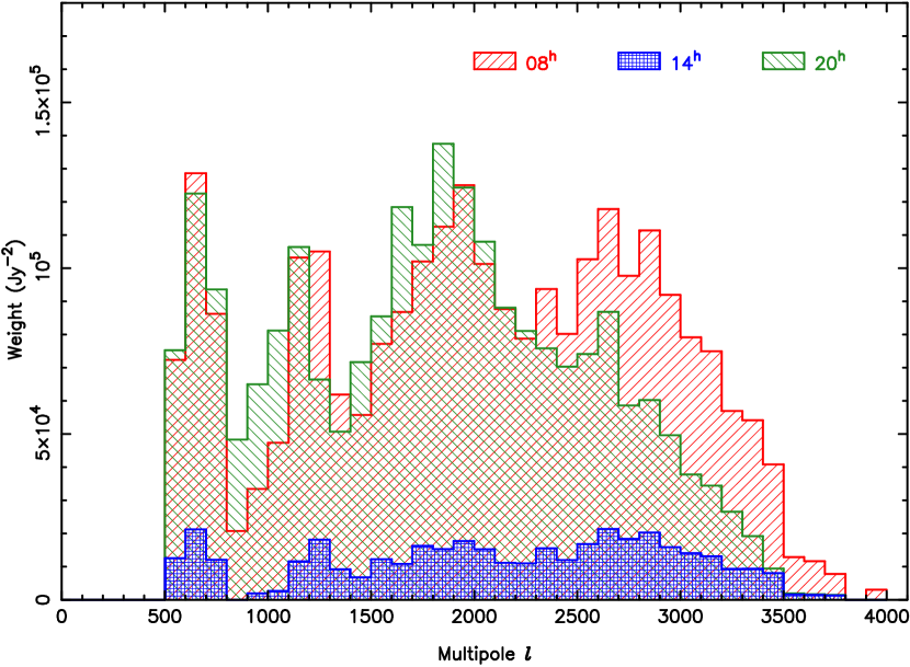
Figure 1.— The distributions of the weights of the visibilities as a function of $\ell$ for the three deep fields. Since the CBI sensitivity does not vary much with baseline or frequency, these weights are roughly proportional to the on sky integration time as a function of $\ell$.

For the observations reported in this paper, four antenna configurations were used. The first configuration, on which the results of Paper I were based, was a ring configuration, with most of the receivers near the perimeter of the platform. This provided fairly uniform $(u,v)$ coverage, many long baselines for robust calibration, and good access to the antennas and instrumentation on the platform during the testing which accompanied initial observations. The second and third configurations were better optimized for the CBI mosaic observations. These more compact configurations provided higher sensitivity in the $\ell=600$–$1500$ range, and were well-suited to low-redshift Sunyaev-Zeldovich observations. In addition, the third configuration provided nearly redundant baselines at different frequencies which enabled us to make a more accurate determination of the radio frequency spectrum of the signals reported in Paper I. The last configuration was an extended configuration with more uniform coverage than the first, more long ($>5\,{\rm m}$) baselines, which are useful for point source monitoring, and greater sensitivity for the frequency spectrum determination out to $\ell=1400$. The distributions of the weights of the data as a function of $\ell$ is shown in Figure 1. The 08h field was observed in the first, second and fourth configurations; the 14h field in the first configuration; and the 20h field in the third configuration.

In the first three configurations, all but one of the receivers were configured to be sensitive to left circular polarization (LCP); the remaining receiver was sensitive to right circular polarization (RCP). In the last configuration all antennas were configured for LCP.

4. Data Analysis

4.1. Calibration and Editing

The equatorial sky coverage and relatively large antennas of the CBI enable us to use a variety of celestial objects as calibrators, including planets, supernova remnants, radio galaxies and quasars. This is convenient for comparing the CBI flux density scale with other measurements (see below) and for accurately calibrating the data. CBI observations are calibrated using nightly measurements of primary calibrators, chosen for their strength and lack of variability at these frequencies (Jupiter, Saturn, Tau A [3C144, the Crab Nebula], and Vir A [3C274]), and a set of secondary calibrators (3C279, 3C273, J1743$-$038, B1830$-$210, and J1924$-$292). Our estimates of the primary calibrator flux densities are based on CBI measurements of these sources relative to Jupiter assuming an apparent Rayleigh-Jeans brightness temperature $T_{\rm Jup}=152\pm 5\,{\rm K}$ at 32 GHz (Mason et al., 1999). This value is uncorrected for the occultation of the CMB by the planet, and applying this correction yields a Rayleigh-Jeans brightness temperature of $154\pm 5\,{\rm K}$. This is also the basis of the Very Small Array calibration (Watson et al., 2002). Since Jupiter is known to have a non-thermal spectrum at these frequencies, and the precise spectral shape is not independently well-determined, this flux density scale is transferred to each of the CBI bands by observations of Tau A, for which the Baars et al. (1977) spectral index $\alpha=-0.299$ is assumed, where $S\propto\nu^{\alpha}$. There is good evidence that the power law index extends to high frequencies (e.g., Mezger et al., 1986). The flux densities of the secondary calibrators are bootstrapped from the nearest primary calibrator observations, and are used when the primary calibrators are either not visible or are too close to the moon. Observations of the primary calibrators over the year 2000 indicate random calibration errors of $\sim 3\%$ night-to-night. The residuals of a polynomial fit to the light curves of the secondary calibrators show a similar scatter. In light of this and the $3.3\%$ calibration uncertainty of the Mason et al. (1999) value for the temperature of Jupiter we assign a calibration uncertainty of $5\%$ to our data. This corresponds to a $10\%$ uncertainty in bandpower (${\rm\mu K^{2}}$). These include the beam uncertainties discussed below.

We have two comparisons of our flux density scale with that of the NRAO Very Large Array (VLA) at 22.4 GHz. First, we compare CBI observations of Mars with the model for the Mars temperature which is used at the VLA (Rudy, 1987), improved by M. Gurwell and B. Butler (private communication, February 2002). R. Perley (private communication, February 2002) has shown that the flux density scale at 22.4 GHz based on this Mars temperature model agrees to within $0.4\%$ with the flux density scale determined at this frequency based on a model of NGC7027 derived by A. van Hoof (private communication, February 2002). The ratio of the temperature of Mars from the CBI to that of the improved Rudy model is $1.026\pm 0.013$. Our second comparison is based on observations of 3C273 on the CBI and the VLA at 7 epochs for which the time interval between observations on the two instruments was small enough to eliminate uncertainties due to source variability. The VLA observations have been calibrated using the improved Rudy Mars model at 22.4 GHz, and the CBI 26–36 GHz measurements have been extrapolated to this frequency. The ratio of the flux density of 3C273 on the CBI to that on the VLA is $0.984\pm 0.010$. From the weighted averages of these two tests we find that the CBI flux density scale, based on the Mason et al. (1999) absolute calibration, is $0.1\%\pm 0.8\%$ lower than the VLA flux density scale at 22.4 GHz. The level of agreement between these two scales is clearly fortuitous, but it does give us confidence that the $5\%$ calibration uncertainty we estimate for the CBI flux density scale is, if anything, conservative.

Individual scans of calibrators and the microwave background are bracketed by measurements of an internal noise calibration source whose equivalent flux density for each baseline and channel is determined by reference to the celestial flux density calibrators. The noise calibration source was initially intended to remove instrumental gain fluctuations over the course of a night, but we found that the instrumental gains were more stable ($\sim 3\%$ rms variations) than the noise calibration source output and so this was not used. This is primarily because of the difficulty in stabilizing the temperature of the noise calibration source amplifier and various other components, all of which lie outside of the cryogenic dewars. All of the (complex) noise calibration source measurements for a given night are averaged together and the data from all baselines are scaled to give an identical response. This removes baseline-based gain and phase calibration errors; it also introduces antenna-based errors which are removed by the subsequent (antenna-based) primary flux density calibration. At the start and end of each night of observing the relative gain and phase errors between the real and imaginary channels were measured using the noise calibration source with and without a $90^{\circ}$ phase shift applied to the receiver local oscillator. The rms quadrature phase is $\sim 5^{\circ}$ and the rms gain errors are $\sim 10\%$. The solutions are stable over a timescale of several weeks.

Lead and trail scans of the CMB fields are interleaved with 1 minute observations of bright ($>1\,\,{\rm Jy}$) nearby calibrators which provide a check on the telescope pointing. From these observations we determine that the absolute rms radio pointing is $\sim 22^{\prime\prime}$, while the rms tracking errors are $\sim 2^{\prime\prime}$.

Data are flagged by both automatic and manual filters. The on-line control system identifies corrupt or potentially unreliable data. These affect periods when the telescope was not tracking properly, a receiver was warm, a local oscillator was not phase locked, the total power of a receiver was out of the normal range, or when a receiver phase-shifter was not acquired. Observer notes were also used to examine periods when there were instrumental problems that might have affected the data quality or there was bad weather, identified by visible cloud cover or corrupted visibilites on the short baselines. A small fraction ($\sim 2\%$) of the data were deleted manually on the basis of these inspections. Subsequent automatic data edits are based on the data scatter and baseline-to-baseline correlations. The first level of rejection is a $5\sigma$ scan-wise outlier edit to eliminate occasional instrumental glitches which give rise to large signals in individual samples. This cut affects a negligible fraction of the data, and our results are not sensitive to the precise level of this cut.

Further automated data-filtering is provided by our differencing procedure, which also generates an accurate estimate of the thermal noise in each scan for each baseline and frequency channel. To do the differencing, individual 8.4-s integrations in the lead and trail scans, which are taken 8 minutes apart, are matched and subtracted. Since our fields are separated by 8 min in observing time, the typical scan length is $\sim 400$ s after slewing and firing the noise calibration source, corresponding to $\sim 50$ integrations of 8.4 s each. In order to prevent a few short scans from biasing the statistics, any scan with fewer than 30 pairs of 8.4 s integrations was rejected. The noise estimates are derived from the differences between the $lead$ and $trail$ fields for individual scans of $\sim 50$ 8.4 sec integrations. Data from different baselines and times which contribute to the same $(u,v)$ points are subsequently combined. This leads to an underestimate of $\sim 8$% in the variance (see Appendix) which we correct for in our statistical analyses and spectrum determinations.

The celestial signals are stationary on an 8-minute timescale, and constant ground signal is cancelled by the ${\it lead}-{\it trail}$ differencing. The noise will be increased by atmospheric noise, ground signal variations, or previously unflagged instrumental anomalies. On this basis any scan for which the rms of the samples is greater than twice the expected thermal noise level is rejected: this primarily eliminates periods affected by weather. Less than $0.1\%$ of the data are rejected by this filter. The noise level is established with reference to data which are clearly free of atmospheric contamination; it is highly repeatable and within $\sim 20\%$ of the expected thermal noise level.

In computing the data differences and thermal noise level, we also compute the covariance between all baseline-channel pairs, i.e., the thermal noise covariance matrix. For the deep 08h field, a single night (2000 January 12) was found to have statistically significant off-diagonal correlations. On this night there were clear instances of atmosphere emission on the short baselines, and the baseline correlations are likely due to poor weather. This day was excluded from the analysis. No anomalous correlations are seen in the deep 14h data. The correlation test on the deep 20h data revealed a single baseline-channel with a large real-imaginary anti-correlation. When this baseline-channel was eliminated from the 20h dataset, no significant baseline-baseline correlations are seen. The excision of these data from the 08h and 20h fields has a negligible effect on the measured power spectrum, suggesting that lower-level, undetected correlator problems of a similar nature also do not affect our result.

The telescope primary beam has been measured accurately using observations of Tau A. The primary beam width (FWHM) is $45.2\times(31\;{\rm GHz}/\nu)$ arc minutes; we estimate a $0.7\%$ uncertainty in the beamwidth. This gives rise to a $1.4\%$ contribution to our overall calibration error. Note that unlike the case for total power experiments, uncertainties in the primary beam width for an interferometer affect only the overall temperature scale, and do not introduce an $\ell$-dependent systematic error. The beam-width measurement is described in Paper III.

4.2. Maximum Likelihood Analysis

4.2.1 Formalism and Algorithms

The determination of the angular power spectrum of the sky from interferometer measurements has been discussed by Hobson et al. (1995) and White et al. (1999); the more general framework of power spectrum estimation is discussed by Bond et al. (1998) and Bond et al. (2000). Here we present a brief overview of our procedure. The details of the method are given in Paper IV. We test a space of hypothetical models for the spectrum, $C_{\ell}$, against the data using the likelihood function as a figure of merit. For complex data points $V$ with zero mean and Gaussian noise described by the covariance matrix ${\bf C}_{jk}$, this is

$$L(C_{\ell})={1\over{\pi^{n}\,{\rm det}\,{\bf C}}}\;{\rm exp}\,\{{\mbox{\boldmath{$-V^{*}$}}}{\bf C}^{-1}{\mbox{\boldmath{$V$}}}\}.$$ (1)

where the covariance matrix, $\bf C$, is given by

$$\mbox{{$\bf C$}}=\mbox{{$\bf C$}}^{\rm N}+\sum_{B}q_{B}\mbox{{$\bf C$}}_{B}^{\rm S}+q_{\rm src}\mbox{{$\bf C$}}^{\rm src}+q_{\rm res}\mbox{{$\bf C$}}^{\rm res}.$$ (2)

Here $\mbox{{$\bf C$}}^{\rm N}$ is the noise covariance and $\mbox{{$\bf C$}}_{B}^{\rm S}$ is the sky (or theoretical CMB) covariance for band $B$. The foreground covariance is made up of $\mbox{{$\bf C$}}^{\rm src}$, a constraint matrix for point sources with known positions, and $\mbox{{$\bf C$}}^{\rm res}$, a matrix which models the contribution of faint point sources of unknown position. The calculation of the expected sky variance $\mbox{{$\bf C$}}_{B}^{\rm S}$ is discussed in many references (e.g., Hobson et al. 1995; Paper I; Paper IV). For a well-designed interferometer the noise term $\mbox{{$\bf C$}}^{\rm N}$ is diagonal (see also § 4.1). The pre-factors $q_{\rm res}$ and $q_{\rm src}$ are held fixed at a priori values (see § 4.3.2). As discussed below, the $q_{B}$ are varied to yield estimates of the microwave background bandpower.

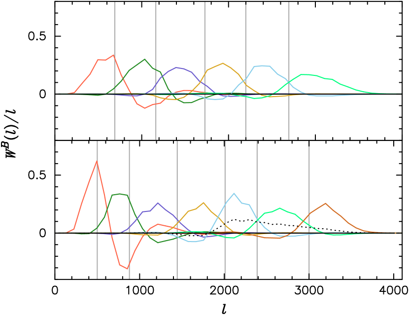
Figure 2.— CBI joint Deep Field window functions. The alternate binning window functions are displayed in the upper panel; the primary binning window functions are displayed in the lower panel. Vertical lines denote the bandpower bin divisions discussed in the text. The window function of the high-$\ell$ rebinning is shown as a dashed line. The expected value of band power for a given spectrum, $C_{l}$, in one bin is $\Sigma_{l}\;W(l)/l\times l(l+1)C_{l}/2\pi$

For the present analysis of the deep field data we adopt a parametric description of the $C_{\ell}$ as seven bins with lower boundaries at $\ell=0$, 500, 880, 1445, 2010, 2388, and 3000. Within each bin, the power spectrum is assumed to be flat in $\ell(\ell+1)C_{\ell}$. The overall amplitudes of the bins $q_{B}$ are treated as free parameters in the maximization of the likelihood. The spacing of $\Delta\ell$ is set by the intrinsic resolution of the CBI in the aperture plane (${\rm\Delta{\ell}}\sim 300$). Here $\Delta\ell$ is the FWHM of the visibility window function (see Paper III). This resolution can be increased by mosaicing. The divisions above were chosen to coincide with breaks in the multi-configuration $(u,v)$ coverage, which minimize correlations between adjacent bins. Given the $(u,v)$-coverage of our data, this choice of binning yields $10$–$15\%$ anti-correlations between adjacent bins. To demonstrate that our results are not sensitive to the choice of bins, we have also conducted the analysis with an alternate set of bins whose boundaries are halfway between those of the primary binning described above (six bins with lower boundaries at $\ell=0$, 690, 1162, 1728, 2199, and 2694). Window functions for each band are shown in Figure 2. These show the sensitivity of a given bandpower bin to power in individual multipoles as a function of $\ell$.

We compute the parameter uncertainties and correlations from the curvature of the likelihood at the best-fit locus. In practice we use the Fisher matrix

$$F_{BB^{\prime}}=\frac{1}{2}{\rm Tr}\left({\bf C}^{-1}\frac{\partial{\mbox{{$\bf C$}}^{\rm S}}}{\partial q_{B}}{\bf C}^{-1}\frac{\partial{\mbox{{$\bf C$}}^{\rm S}}}{\partial q_{B^{\prime}}}\right)$$ (3)

as a computationally efficient estimator of the curvature. In the approximation that the likelihood function is Gaussian, $F_{BB^{\prime}}^{-1}$ is the correlation matrix of the fitted parameters. As a check on the Fisher matrix results, we have also mapped the likelihoods in individual bands and checked against the error bars computed in the offset log-normal approximation (Bond et al., 2000). We find good agreement between these three methods. Monte Carlo tests of simulated CBI data show that these error estimates, as well as the bandpower estimates themselves, are unbiased.

The dominant foreground for the CBI is composed of discrete extragalactic radio sources described by the correlation matrices $\mbox{{$\bf C$}}^{\rm res}$ and $\mbox{{$\bf C$}}^{\rm src}$. For purposes of this analysis we neglect other possible foregrounds, although see § 5 for limits on the possible contribution of foregrounds on large angular scales.

4.2.2 Implementation

Since in the small-angle limit interferometers directly measure linear combinations of the sky Fourier modes, the extraction of angular power spectra from the data is in principle simpler than in the case of total power experiments. In general, however, $\mbox{{$\bf C$}}_{jk}$ has non-negligible off-diagonal elements, and depending on the $(u,v)$-sampling of the dataset this matrix can be large. To deal with the computational challenge of inverting this matrix, we have developed a Fourier gridding algorithm. This algorithm constructs a data vector composed of linear combinations of the visibility data and calculates the resulting covariance matrix. For single-field analyses such as we report here, the primary effect of this gridding is to reduce redundancies in the $(u,v)$-dataset caused by dense aperture plane sampling. This compression is typically a factor of 3 to 4: for each field there are several thousand visibilities, which are gridded down to 970 estimators. This results in over an order of magnitude increase in the speed of the likelihood analysis. This pipeline and the associated formalism are discussed in Paper IV.

The pipeline was implemented on the 4 and 32 processor shared memory Alpha GS320 and ES45 clusters at CITA. The codes were parallelized using Open MP directives. A complete joint analysis of the three deep fields takes approximately 4 CPU hours. This includes pre-gridding and the calculation of all ancillary quantities such as the bandpower window functions, likelihood maps and noise spectra. Bandpower estimates can be obtained in as little as 1 CPU hour for the deep field data. These rapid turnaround times permitted extensive testing of the data and pipeline; results of some of these tests are discussed in §4.4.

4.3. Discrete Sources

Extragalactic radio sources are the dominant foreground to CMB observations over the 26–36 GHz frequency band on arcminute scales (Tegmark & Efstathiou, 1996). If no allowance for this foreground is made, the few brightest discrete sources in each field dominate any power spectrum determination beyond $\ell\sim 1000$. While much is known about radio source populations at lower frequencies, this is not the case at 31 GHz, and observations at this frequency are essential in dealing with the point source contamination at high $\ell$. We therefore constructed a 26–34 GHz receiver for the OVRO 40 meter telescope which we have used to study the source population at this frequency and to provide a direct check on the CBI calibration. We have also computed 31 GHz source counts directly from the CBI deep maps, and the mosaic maps presented in Paper III. The results from these complementary approaches are presented in § 4.3.1. These results form the basis of our strategy for dealing with both the bright sources and the statistical residual source background. The treatment of radio sources in the CMB analysis is detailed in § 4.3.2.

4.3.1 31 GHz Radio Source Measurements

Table 2Subtracted Discrete Sources

Name	R.A. (J2000)	Decl. (J2000)	$S_{31}$ (mJy)	Field	$r$ (arcmin)	$S_{\rm CBI}$ (mJy)
084204-0317	08:42:04.110	-03:17:06.9	$6.0\pm 1.4$	C08(L)	39.7	0.5
084242-0344	08:42:42.690	-03:44:25.8	$8.7\pm 1.9$	C08(L)	45.3	0.3
084336-0302	08:43:36.940	-03:02:59.5	$7.9\pm 1.2$	C08(L)	17.3	5.3
084533-0217	08:45:33.200	-02:17:31.4	$6.4\pm 1.5$	C08(L)	54.1	0.01
084553-0305	08:45:53.200	-03:05:38.4	$9.1\pm 1.8$	C08(L)	18.8	5.7
084553-0342	08:45:53.740	-03:42:02.3	$9.0\pm 2.0$	C08(L)	37.0	1.2
084730-0251	08:47:30.490	-02:51:36.6	$6.5\pm 1.2$	C08(L)	46.5	0.2
084732-0340	08:47:32.920	-03:40:39.7	$42.6\pm 1.9$	C08(L)	53.0	0.1
084803-0257	08:48:03.110	-02:57:52.4	$20.7\pm 1.6$	C08(L)	52.3	0.1
084944-0317	08:49:44.490	-03:17:59.2	$47.3\pm 1.9$	C08(T)	44.7	1.8
085311-0342	08:53:11.900	-03:42:48.1	$8.0\pm 1.4$	C08(T)	33.8	1.6
085322-0259	08:53:22.310	-02:59:48.7	$7.8\pm 1.4$	C08(T)	14.7	5.9
085326-0211	08:53:26.340	-02:11:49.3	$9.4\pm 2.3$	C08(T)	59.3	0.01
085328-0341	08:53:28.250	-03:41:08.0	$41.4\pm 1.1$	C08(T)	33.4	8.4
085329-0258	08:53:29.860	-02:58:04.3	$7.0\pm 1.6$	C08(T)	17.3	4.7
085359-0302	08:53:59.440	-03:02:56.6	$15.0\pm 2.6$	C08(T)	21.1	8.3
085430-0223	08:54:30.480	-02:23:14.9	$17.8\pm 1.5$	C08(T)	54.3	0.03
144019-0308	14:40:19.430	-03:08:34.5	$8.5\pm 1.7$	C14(L)	48.5	0.1
144042-0406	14:40:42.950	-04:06:47.3	$9.4\pm 1.7$	C14(L)	25.6	3.9
144254-0329	14:42:54.290	-03:29:34.8	$7.0\pm 1.4$	C14(L)	24.5	3.1
144400-0259	14:44:00.070	-02:59:20.3	$6.4\pm 1.5$	C14(L)	58.9	0.01
144444-0400	14:44:44.990	-04:00:47.7	$9.8\pm 1.8$	C14(L)	42.7	0.5
144445-0311	14:44:45.870	-03:11:51.1	$9.1\pm 1.8$	C14(L)	56.4	0.01
144457-0312	14:44:57.220	-03:12:03.4	$30.9\pm 3.0$	C14(L)	58.4	0.03
144459-0311	14:44:59.650	-03:11:04.1	$11.9\pm 2.4$	C14(L)	59.5	0.02
144506-0326	14:45:06.230	-03:26:13.4	$15.5\pm 3.3$	C14(L)	52.4	0.06
144542-0329	14:45:42.430	-03:29:57.4	$41.3\pm 2.9$	C14(L)	59.2	0.05
144824-0316	14:48:24.510	-03:16:47.1	$6.1\pm 1.4$	C14(T)	40.9	0.5
144933-0352	14:49:33.660	-03:52:19.2	$22.1\pm 3.7$	C14(T)	7.0	20.7
144954-0302	14:49:54.240	-03:02:36.7	$21.9\pm 2.8$	C14(T)	47.4	0.4
145146-0356	14:51:46.180	-03:56:53.7	$26.1\pm 1.8$	C14(T)	27.5	9.2
145207-0325	14:52:07.080	-03:25:04.1	$7.8\pm 1.4$	C14(T)	40.4	0.6
145230-0315	14:52:30.250	-03:15:35.2	$6.7\pm 1.0$	C14(T)	51.0	0.05
204542-0323	20:45:42.330	-03:23:03.6	$13.0\pm 2.2$	C20(L)	45.0	0.5
204603-0336	20:46:03.810	-03:36:47.3	$11.1\pm 1.8$	C20(L)	39.7	1.0
204608-0249	20:46:08.670	-02:49:39.2	$11.7\pm 1.4$	C20(L)	55.4	0.01
204645-0316	20:46:45.400	-03:16:15.1	$9.2\pm 2.0$	C20(L)	31.8	2.2
204710-0236	20:47:10.320	-02:36:22.7	$197.7\pm 1.9$	C20(L)	58.1	0.2
204731-0356	20:47:31.600	-03:56:11.5	$6.4\pm 1.4$	C20(L)	31.3	1.6
204745-0246	20:47:45.660	-02:46:05.0	$79.7\pm 1.6$	C20(L)	46.0	2.3
204800-0243	20:48:00.130	-02:43:03.7	$9.4\pm 1.1$	C20(L)	48.0	0.2
204830-0428	20:48:30.610	-04:28:20.3	$7.0\pm 1.7$	C20(L)	58.4	0.01
205001-0249	20:50:01.360	-02:49:06.0	$14.9\pm 2.4$	C20(L)	45.7	0.5
205038-0305	20:50:38.860	-03:05:59.1	$39.4\pm 2.5$	C20(L)	38.2	4.5
205041-0249	20:50:41.330	-02:49:17.0	$15.9\pm 3.3$	C20(L)	50.8	0.1
205045-0337	20:50:45.050	-03:37:43.3	$15.2\pm 2.7$	C20(L)	32.3	3.5
205355-0259	20:53:55.400	-02:59:43.2	$10.3\pm 1.3$	C20(T)	51.2	0.06
205520-0306	20:55:20.170	-03:06:17.5	$6.0\pm 1.4$	C20(T)	31.0	1.6
205543-0350	20:55:43.650	-03:50:51.6	$32.3\pm 2.1$	C20(T)	25.2	13.6
205550-0416	20:55:50.260	-04:16:46.8	$180.7\pm 4.5$	C20(T)	48.4	2.8
205735-0250	20:57:35.150	-02:50:49.5	$14.6\pm 3.1$	C20(T)	41.5	1.0
205812-0312	20:58:12.410	-03:12:26.0	$6.3\pm 1.0$	C20(T)	29.1	2.0
205822-0303	20:58:22.070	-03:03:26.8	$6.0\pm 1.2$	C20(T)	36.9	0.8
210000-0343	21:00:00.370	-03:43:02.8	$11.0\pm 2.4$	C20(T)	51.8	0.05
210007-0325	21:00:07.950	-03:25:43.7	$12.9\pm 2.9$	C20(T)	52.3	0.05
210029-0317	21:00:29.510	-03:17:41.6	$8.8\pm 2.1$	C20(T)	58.8	0.01

The OVRO 40-meter telescope was used at 31 GHz to survey the $2225$ NVSS sources brighter than $S_{1.4\,{\rm GHz}}=6\,{\rm mJy}$ in four 22.5 square degree fields which encompass the deep and mosaic fields. With the $4\sigma$ cutoff specified below, the survey has a $7\%$ chance of one or more false detections. To minimize the effects of variations in the flux density of the monitored sources, the 40-meter and CBI observations were made as nearly as possible over the same period of time. The typical sensitivity achieved on the 40-meter telescope was $2\,{\rm mJy}\,({\rm rms})$, although the distribution extends to $5\,{\rm mJy}$. $12\,\%$ of the targeted NVSS sources were detected above the survey thresholds of $4\sigma$ and $S_{\rm min,31}=6\,\,{\rm mJy}$. The survey is $90\%$ complete at $S_{31}>16\,{\rm mJy}$ and $99\%$ complete at $S_{31}>21\,{\rm mJy}$. The 56 detected sources within 1 degree of the lead or trail field centers were subtracted directly from the CBI data; these sources are shown in Table 2. This table lists total flux densities, $S_{31}$; distances in arc minutes from the center of the CBI field, $r$; and the flux density predicted on the CBI including the effects of the CBI primary beam, $S_{\rm CBI}$. Few of these 56 sources contribute significantly to the data since most of them are too distant from the CBI field centers to do so: in each deep field only a few sources are visible in the images. The spectral indices of these sources were computed by comparison with the NVSS 1.4 GHz flux densities, and we find $\bar{\alpha}=-0.45$ with an rms dispersion of 0.37; the minimum and maximum spectral indices were $-1.32$ and $+0.50$.

We have used the CBI deep and mosaic maps to determine the source counts at 31 GHz. To do this, we made maps from the long baseline ($>250\,\lambda$) data and searched for peaks over the $5\sigma$ threshold. Below this level the probability of false detections is significant. A fit to the resulting counts over the range $5$–$50$ mJy yields

$$N(>S_{31})=2.8\pm 0.7\,{\rm deg^{-2}}\,\left(\frac{S_{31}}{10\,\,{\rm mJy}}\right)^{-1.0}$$ (4)

This is slightly higher than the 31 GHz counts estimated from either the NVSS counts or the 15 GHz counts of Taylor et al. (2001). In both the deep and mosaic maps no sources were detected above the $5\sigma$ limit which were not NVSS objects. The area searched depends on the limiting flux density chosen: in the deep maps the area was 6 square degrees at 12 mJy, falling to 1.8 square degrees at 6 mJy. In the mosaic maps the area was 47 square degrees at 25 mJy, falling to 12.2 square degrees at 18 mJy. The flux densities of the sources detected in both the deep and mosaic maps are consistent with the OVRO determinations, with the agreement typically within $5\%$.

As discussed above, the OVRO-detected bright sources were directly subtracted from the CBI data since the OVRO source subtraction is a step in the standard data-analysis pipeline which has been useful in producing diagnostic images of the data. In § 4.3.2 we discuss a method (the constraint matrix approach of Halverson et al. 2002) of dealing with point source foregrounds which does not require knowledge of the source flux densities. We find that this method applied to the OVRO sources gives very similar results as direct subtraction. These complementary techniques of dealing with this bright source population have been useful in extending our power spectrum measurments to the instrumental limit of 3500.

4.3.2 Statistical Treatment of Sources

In addition to the brightest sources in the CBI fields, which have been measured and subtracted with the OVRO data, we must deal with sources too faint to measure directly but which contribute statistically to our measurements. Since most radio sources have spectra which fall towards higher frequencies, and since there are wide-area radio sky surveys at lower frequencies with sensitivities comparable to what we have in the CBI deep field maps, most of the sources which contribute are readily identified from the low-frequency surveys. For this purpose we use the NVSS. There is also a small contribution due to sources which are too faint to appear even in NVSS. We call these latter “residual” sources and estimate their contribution from the CBI 31 GHz source counts.

After the subtraction of the bright sources monitored at OVRO, there remain three components of point source contamination: one due to data correlations induced by the (imperfect) OVRO source subtraction; a component due to the NVSS sources whose positions are known, but whose flux densities are not measured at 31 GHz; and a residual component due to sources whose contribution must be estimated from source counts. These are represented as

$$q_{\rm OVRO}\mbox{{$\bf C$}}^{\rm OVRO}+q_{\rm NVSS}\mbox{{$\bf C$}}^{\rm NVSS}+q_{\rm res}\mbox{{$\bf C$}}^{\rm res}$$ (5)

The $q$ are prefactors which are held fixed in the bandpower fit, and allow for the effect of overall uncertainties in our estimates of the source covariances. If $q=1$, an extra amount of variance equal to the variance assumed in the calculations of the source covariance matrices is allowed in each source mode. In the limit $q\rightarrow\infty$ the data modes corresponding to the point sources are completely removed from the data, i.e., these modes are “projected out” (Halverson et al., 2002; Bond et al., 1998). We note that it is possible to allow the $q$ to be free parameters in the fit, and we do not find significantly different results in this case; however it is more conservative to fix the $q$ at very large values. Explicit procedures for calculating the three source covariances matrices are discussed in Paper IV.

We adopt the strategy of projecting the modes corresponding to OVRO residuals and NVSS sources out of our data. A nominal variance is assigned to each source based on the OVRO measurement uncertainty or, for the NVSS sources, the width of the OVRO-determined 1.4 to 31 GHz spectral index distribution. We then set $q_{\rm OVRO}=q_{\rm NVSS}=30$ which projects these modes out of the data. We find that our power spectra at high $\ell$, where point sources are most troublesome, are little affected by variations in $q$ between $q=30$ to $q=10^{6}$.

At significantly larger values of $q$ the matrices are numerically ill-conditioned. We have tested the source projection algorithm extensively on both real and simulated data and find that it is robust against, for instance, randomly reassigning estimated variances between sources and randomly perturbing the source positions assumed in the projection by $30^{\prime\prime}$ (rms).

We model the contribution of the residual sources ($\mbox{{$\bf C$}}^{\rm res}$) as a Gaussian white-noise foreground. We determine the normalization of this matrix from Monte Carlo simulations assuming the source counts presented in § 4.3.1 to generate random populations at 31 GHz. Since at fainter flux levels the counts are expected to flatten somewhat, we used a slightly shallower slope for the counts ($N(>S)\propto S^{-0.875}$) for this calculation, although at the $1\sigma$ level our result is consistent with that obtained for $N(>S)\propto S^{-1}$. In order to determine what fraction of these sources fall below the NVSS detection threshold of 3.4 mJy and hence are residual, the sources are extrapolated down to 1.4 GHz using the observed OVRO-NVSS distribution of spectral indices (with $\bar{\alpha}=-0.45$ — see § 4.3.1). Since the OVRO survey is strongly biased towards flat-spectrum sources this will overestimate the residual source power level. We find a 31 GHz variance of $C_{0}^{\rm res}=0.08\,{\rm Jy^{2}\,sr^{-1}}$. We get a similar result, $C_{0}^{\rm res}=0.10\,{\rm Jy^{2}\,sr^{-1}}$ from the analytic calculation described in Paper IV. In our highest bin this corresponds to a power level of $\sim 115\,{\rm\mu K^{2}}$, which is less than the thermal noise in this bin and all others; we assign an uncertainty of $50\%$ to this value, corresponding to $\pm 0.04\,{\rm Jy^{2}\,sr^{-1}}$ ($57\,{\rm\mu K^{2}}$). This uncertainty is based on varying the number counts and spectral index parameters within the range allowed by their uncertainties, and rerunning the Monte Carlo simulations used to calculate the residual power. Comparable power levels are obtained if, instead of using the 31 GHz counts, we extrapolate in frequency from the 1.4 GHz number counts using a simple Gaussian model for the spectral index distribution which is constrained to reproduce the detection statistics observed in the OVRO survey. As a test on the robustness of this correction we re-ran the power spectrum analysis doubling the NVSS/residual source threshold from 3.4 to 6.8 mJy at 1.4 GHz with similar results. The number density of the residual sources on the sky is too high to permit full projection of these data modes, and in any case their positions are not known so this would be impossible. We therefore fix $q_{\rm res}=1$, which approximately corresponds to subtracting our conservative estimate of the residual source power level from the spectrum.

The cost of projecting out the NVSS sources is a loss of sensitivity of the CBI at high $\ell$ due to our limited knowledge of the faint point sources at 31 GHz. The best way to address this problem in the near term is with a sensitive 31 GHz receiver on the NRAO Green Bank Telescope (GBT). Such an instrument is under construction and should be in use by the end of 2003.

4.4. Data Consistency Tests

The redundancy of observations on the CBI deep fields allows many checks on the dataset. Below we describe the key tests performed.

4.4.1 $\chi^{2}$ Tests

A simple and direct test of the data consistency is provided by computing the $\chi^{2}$ of visibilities with the same $(u,v)$ coordinate, frequency, and sky pointing. We compared the data at each $(u,v)$ point on each night with the average of all other nights. This procedure identified three days on the deep 20h field which were formally inconsistent with the total dataset. We exclude these days from the analysis, which has a small ($\ll 1\sigma$) effect on our results. The visibilities for all other days were consistent with the estimate of the visibilities from the rest of the data. A typical value of the $\chi^{2}$ of an individual day as compared with the rest of the dataset is $\chi^{2}/\nu=0.986$ with $\nu=1617$. For such a day the probability of exceeding this value under the null hypothesis is 65%.

The data on each configuration of each field was also subdivided in half by time, subtracted, and then compared in this manner. The $\chi^{2}/\nu$ values for these tests on the 08h data (3 configurations), and the 14h, and 20h data (each one configuration) were $0.990$, $0.993$, $0.967$, $1.015$, and $0.986$ for $\nu=2310$, $2710$, $3948$, $2310$, and $4848$, respectively. These results indicate that our estimate of the thermal noise variance is correct to within $\sim 2\%$.

4.4.2 Kolmogorov-Smirnov Tests

We have used the Kolmogorov-Smirnov (KS) test to determine if the visibility data are consistent with a Gaussian distribution. This is the expectation when the signal-to-noise-ratio per baseline-channel combination is low, as is the case for the $\ell>1000$ data on any given field once the bright point sources have been subtracted. The quantity of interest is the ratio of the visibility to its estimated uncertainty

$$t=\frac{V}{\sigma_{V}}$$ (6)

If the $\sigma_{V}$ were known a priori then $t$ would have a Gaussian distribution with unit dispersion. As discussed in the Appendix, however, this is not the case, and a $4\%$ correction to the expected standard deviation ($\sigma_{t}$) of $t$ is required. Furthermore, as discussed in § 4.4.1, we have only determined that our measurements of the thermal noise are accurate at the $1\%$ level. We therefore apply the KS test to the data under the null hypothesis that the observed distribution of $t$ is consistent with a Gaussian distribution of zero mean and $\sigma_{t}=1.04$, but vary $\sigma_{t}$ by $\pm 1\%$ for each dataset. We find good consistency with the Gaussian distribution, so to the accuracy that the noise level has been well-quantified we do not detect significant non-Gaussianity in the visibility data.

4.4.3 Power Spectra

Two sets of bandpowers $q_{1,B}$ and $q_{2,B}$ (i.e., two power spectrum estimates) can be compared for consistency by forming

$$\chi^{2}=(q_{1,B^{\prime}}-q_{2,B^{\prime}})^{T}\,(F^{-1}_{1,BB^{\prime}}+F^{-1}_{2,BB^{\prime}})^{-1}\,(q_{1,B}-q_{2,B}).$$ (7)

Under the hypothesis that the likelihood function is Gaussian and the $q_{i,B}$ are drawn from the same underlying power spectrum with noise correlations specified by the elements of the inverse of the Fisher matrices $F^{-1}_{i,BB^{\prime}}$, this is distributed as $\chi^{2}$ with $\nu$ degrees of freedom, where $\nu$ is the number of free parameters in each spectrum estimate (7). The $\chi^{2}/\nu$ values (and significances) for the 08h/14h, 08h/20h, and 14h/20h power spectrum comparison are, respectively, $1.40$ ($20\%$), $1.03$ ($40\%$), $1.08$ ($38\%$).

4.4.4 Undifferenced and Doubly-Differenced Power Spectra

In order to estimate the level of non-celestial signals which we are removing from the data, we have extracted the power spectra of the undifferenced data (i.e., no ${\it lead}-{\it trail}$ based ground subtraction). The power spectrum estimates derived from the shortest baselines show the effect of ground-spillover, but at $\ell>600$ they are within a factor of $\sim 4$ (in $\mu$K) of the differenced spectrum, and are seen to fall strongly with increasing $\ell$. Since the CMB signals on the short baselines are up to a factor of $\sim 10^{3}$ (in $\mu$K) less than the ground signal on these baselines, the low power levels in the undifferenced spectrum indicate that the signal averages down when data from many days and position angles are combined. At multipoles $\ell>1000$ the undifferenced signal is within $\sim 1\sigma$ of the differenced spectrum except in a single bin. In this bin ($2388<\ell<3000$) the undifferenced power level was originally found to be about twice the thermal noise level. This was traced to correlator offsets in a single channel on several baselines. Since the $\chi^{2}$ of the differenced data on these baselines are consistent within the noise with data from other baselines and the power spectrum is not significantly affected by the exclusion of the channel in question, we infer that the contamination is effectively removed by our differencing procedure.

We have also divided the data from the lead and trail pointings for each field in half, subtracted these, and derived the power spectrum of the combination of the doubly-differenced data sets for the three fields. This is consistent with zero — $\chi^{2}/\nu=1.06$ for $\nu=7$ DOF (7 bins).

4.4.5 Simulated Datasets

We carried out a series of Monte Carlo tests on the data. In these tests, the individual days that went into the deep field datasets for which we have high sensitivity, 08h and 20h, were resampled with the observed $(u,v)$ coverage and noise assuming a known input power spectrum. Since the signal to noise ratio beyond $\ell\sim 1000$ in a single day is very low, we extracted only the first two bandpowers from each day and its corresponding simulated dataset. We find that the distribution of the bandpowers of the real data is consistent with that of the simulated data. The distribution of the rms powers of the real data within the primary beam area on the dirty maps is likewise consistent with that of the simulated data.

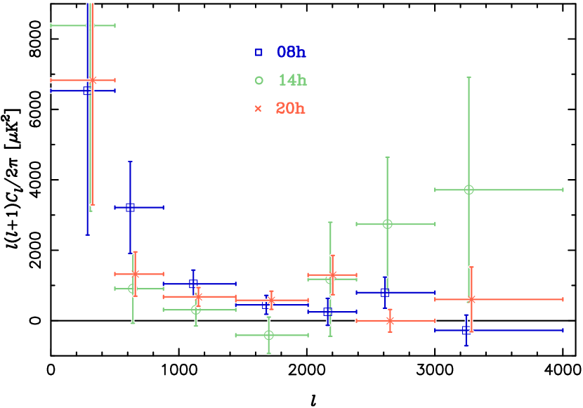
Figure 3.— Power spectra from the individual CBI deep fields shown for the primary binning only. The 08h, 14h, and 20h data are denoted by squares (blue), circles (green), and crosses (red), respectively. The horizontal location of each point on the power spectrum is $\ell_{\rm eff}$ and the horizontal error bars indicate the full extent of each band.

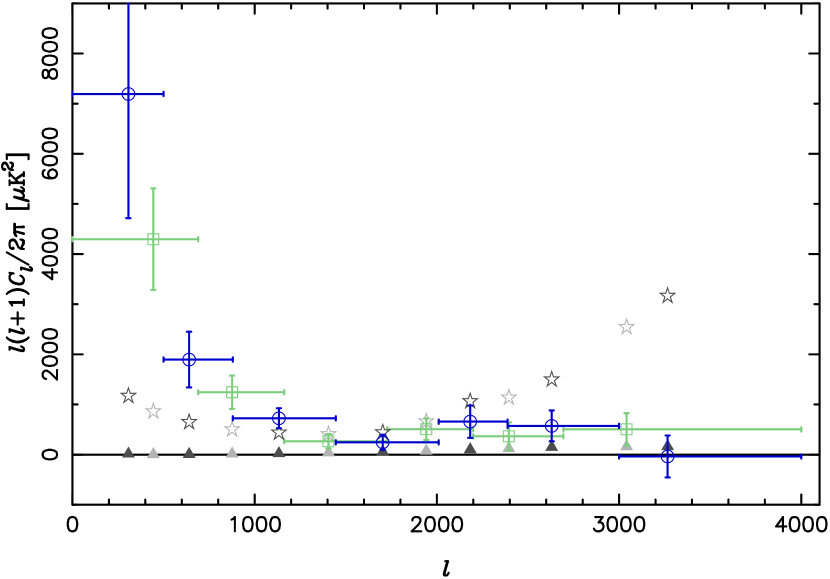
Figure 4.— Joint CBI deep field power spectra for the primary (blue open circles) and alternate (green open squares) binnings. The placement of the points in $\ell$ is determined as in figure 3. Also shown are the thermal noise power spectrum (open stars) and the residual source power spectrum (solid triangles).

Table 3Deep Field Bandpower Data $({\rm\mu K^{2}})$

Bin	$\ell_{\rm eff}$	Joint	deep 08h	deep 14h	deep 20h
$0-500$	307	$7193\pm 2478$	$6531\pm 4100$	$8381\pm 5274$	$6829\pm 3540$
$500-880$	640	$1896\pm 556$	$3213\pm 1306$	$910\pm 983$	$1322\pm 627$
$880-1445$	1133	$724\pm 200$	$1045\pm 389$	$310\pm 461$	$674\pm 264$
$1445-2010$	1703	$245\pm 149$	$449\pm 266$	$-415\pm 516$	$578\pm 257$
$2010-2388$	2183	$657\pm 323$	$251\pm 382$	$1174\pm 1620$	$1293\pm 557$
$2388-3000$	2630	$573\pm 308$	$795\pm 442$	$2742\pm 1897$	$-5\pm 320$
$3000-4000$	3266	$-37\pm 418$	$-276\pm 435$	$3717\pm 3195$	$604\pm 920$

5. Results

The power spectra of the individual deep fields are shown in Figure 3. These illustrate the field-to-field consistency of power spectra discussed in § 4.4.3. Figure 4 shows the results for the joint fields, as well as the thermal noise and residual source power spectra. It is evident that the residual source correction is small compared to the observed power levels, and that errors in the thermal noise level power spectrum at the $1\%$ level indicated in § 4.4.1 are also small compared to observed power levels over the entire $\ell$-range. The bandpower results are summarized in Table 3. In this Table, $\ell_{\rm eff}$ denotes the centroid of the bandpower window function. The error bars in this table are $1\sigma$

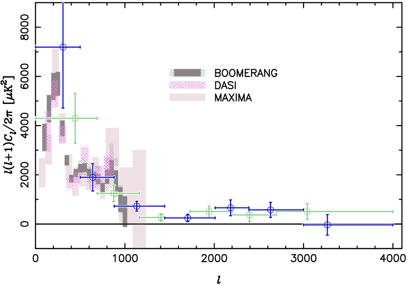
Figure 5.— Comparison of the CBI deep field power spectrum with BOOMERANG (Netterfield et al., 2002), DASI (Halverson et al., 2002), and MAXIMA (Lee et al., 2001) results. The rectangles indicate the 68% confidence intervals on band-power; for BOOMERANG, the solid rectangles indicate the 68% confidence interval for the statistical and sample variance errors, while the hatched rectangles shows the amount by which a $\pm 1\sigma$ error in the beamwidth ($12\farcm 9\pm 1\farcm 4$) would shift the estimates (all up or all down together). Results from the CBI primary binning are shown as blue open circles, and the alternate binning results are shown as green open squares. The high value of the power seen in the first bin of the primary and alternate binnings relative to other observations has rather low significance ($\sim 1.7\sigma$) due to the large sample variance in the deep field spectra at low $\ell$; this is discussed further in the text.

Figure 5 compares the CBI deep field results directly with the BOOMERANG, DASI, and MAXIMA data. We see that there is good agreement between all the observations in the range $\ell\sim 600\rightarrow 1000$, but that the CBI deep field observations are somewhat higher than the other experiments in the range $\ell<600$. This discrepancy— which is not statistically significant— is discussed further below and in § 6. We see in this figure that the power level drops significantly in the range $\ell\sim 500\rightarrow 2000$, confirming the results of Paper I, which were based on a subset of these data, and extending the region in $\ell$-space over which this drop occurs to higher $\ell$. Above $\ell\sim 2000$ the level of power is flat and significantly greater than zero, contrary to what is expected from standard models of the intrinsic anisotropy. We return to this point in §5.2.

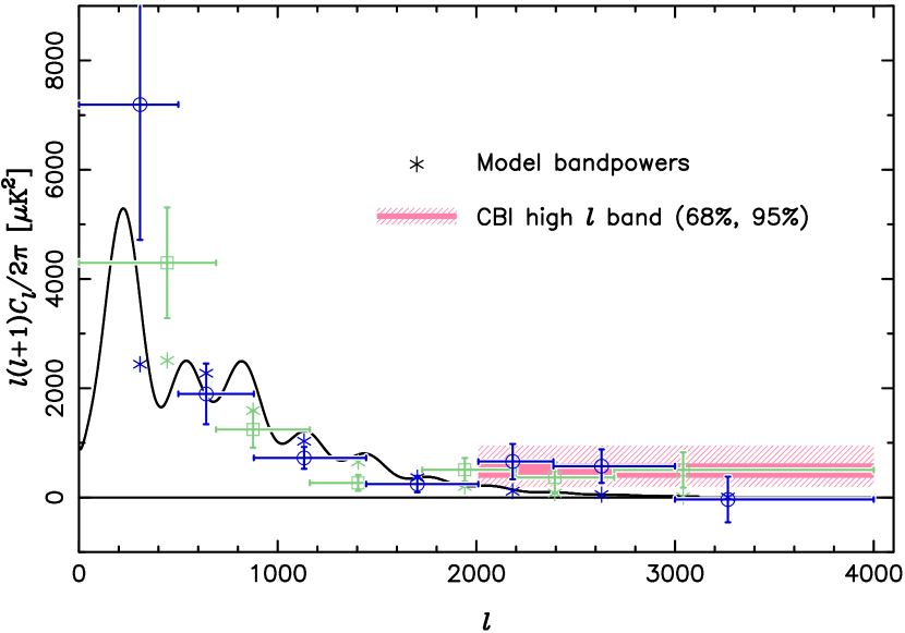
Figure 6.— The CBI deep field power spectrum: Results from the CBI primary binning are shown as circles, and the alternate binning results are shown as squares. The shaded region shows the 68% and 95% central confidence intervals for the high-$\ell$ CBI bin $2000<\ell<4000$; these was computed by combining the last three primary bins into a single bin in bandpower and mapping the likelihood of this band, marginalizing over irrelevant parameters. The curve shows the spectrum derived in Paper V as a best fit to “all-data” (Boomerang, CBI, DASI, DMR, Maxima, VSA and earlier observations) using strong priors (age of the universe $>10$ Gyr, $45\;{\rm km\,s^{-1}\,Mpc^{-1}}<{H_{0}}<90\;{\rm km\,s^{-1}\,Mpc^{-1}}$, zero curvature, plus large scale structure constraints). Stars show the expected signal in each CBI band for this model. The power in the range $\ell\sim 2000\rightarrow 3500$ differs from the best fit model at the $3.1\sigma$ level. This excess power is discussed further in the text.

In Figure 6, we have plotted the CBI deep spectrum together with the best-fit model to the CBI mosaic results combined with the BOOMERANG, DASI, MAXIMA, VSA and earlier observations (“all-data”), derived in Paper V, subject to the constraints listed in the figure caption. Here we also show the expected level of the CBI deep spectrum in the primary and alternate binnings obtained by integrating this model over the CBI window functions shown in Figure 2. We find that the CBI deep spectrum is reasonably consistent with the theoretical curve at $\ell<1000$ — the first two bins of the standard binning yield $\chi^{2}/\nu=1.86$ (84% significance) to the theoretical curve, and the first two bins of the alternate binning yield $\chi^{2}/\nu=2.03$ ($87\%$ significance).

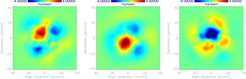
Figure 7.— Wiener-filtered images of the 08h, 14h and 20h deep fields (see § 8 of Paper IV). The positions of the field centers are given in Table 1. The dominant features in these images have angular scales $\sim 15\arcmin$, and are due to structures with multipoles observed on $\sim 1$ meter baselines, which span the range of the second and third acoustic peaks. The approximate fraction of the data contributing to these features can be seen in Figure 1, where the peaks in the range $500<\ell<800$, correspond to the data contributing to the dominant features in these images. Due to the differencing and the sidelobes of the point spread function, there is some ambiguity in relating particular features in these raw maps to actual features on the sky. Figure 1 of Paper I presents a similar image of the 08h field, along with the point spread function and one of several possible deconvolutions.

We have constructed Wiener-filtered images of the sky signal in which we have subtracted the point source and noise contributions by the method described in Paper IV and in Bond et al. (1994). The images for the three fields are shown in Figure 7.

5.1. Limits on Diffuse Foregrounds

We can use the spectral coverage of the CBI to place limits on potentially contaminating foregrounds such as Galactic synchrotron ($\alpha\sim-0.7$) and free-free emission ($\alpha\sim 0$). To do this, we generated a set of 100 realizations of our data set using the best-fit power spectrum shown in Figure 6, as well as 100 realizations of a foreground with zero spectral index, typical of free-free emission, with a flat power spectrum. We added the two sets together at various power levels of the foreground, and fitted the data from $\ell<800$, where we are most sensitive to the spectral index, to a two-bin ( $\ell<500$ and $\ell>500$) model with a varying spectral index, finding a single best-fit spectral index using that model. Models containing both CMB and foreground components are too ill-constrained by the data to be useful. We find that the mean best-fit spectral index for the zero-foreground simulations is 1.97, and that the scatter of the individual simulations is 0.34. Furthermore, we find that the mean best-fit spectral index at different simulation power levels is well described (1% error) by taking the means of the CMB and foreground spectral indices, weighted by their power levels.

$$\alpha_{\rm fit}=\frac{\alpha_{\rm cmb}P_{\rm cmb}+\alpha_{\rm fg}P_{\rm fg}}{P_{\rm cmb}+P_{\rm fg}},$$ (8)

with $P_{\rm cmb}=2455\,\mu{\rm K}^{2}$ and $\alpha_{\rm cmb}=1.97$ for $500<\ell<800$. The data give a best-fit spectral index of $1.84\pm 0.34$, $0.4\,\sigma$ from the zero-foreground value. The $1\sigma$ upper limit for $\ell<880$ on a free-free like foreground contribution is $\alpha_{\rm fit}=1.84-0.34=1.50$, which, using Eq 8, yields $P_{\rm fg}=744\,\mu{\rm K}^{2}$ ($31\%$ of $P_{\rm cmb}$) for $\alpha_{\rm fg}=0$. For a synchrotron spectral index of $-0.7$, we get an upper limit $P_{\rm fg}\leq 521\,\mu{\rm K}^{2}$ $(P_{\rm fg}<21\%$ of $P_{\rm cmb})$.

5.2. The Apparent Excess Power at High $\ell$

An interesting feature of the joint spectrum is the apparent excess power observed above $\ell=2000$. To quantify this, we reanalyzed the data with the last three bins in the primary binning grouped into a single bin ($2010<\ell<4000$). For the single high-$\ell$ bin we obtain a best-fit bandpower of $508\,{\rm\mu K^{2}}$ with an uncertainty (from the Fisher matrix) of $168\,\mu{\rm K}^{2}$. In order to more accurately estimate the uncertainty we have calculated the likelihood curve of the bandpower in the high-$\ell$ bin explicitly— marginalizing over the bandpower in the previous bin, which is the dominant bandpower correlation, and the residual source correction— and integrated the likelihood function to determine confidence intervals. The $68\%$ and $95\%$ central confidence intervals are, respectively, $(359\rightarrow 624)\,{\rm\mu K^{2}}$ and $(199\rightarrow 946)\,{\rm\mu K^{2}}$. Averaged over the high-$\ell$ bin, the model shown in Figure 5 predicts $\sim 66\,{\rm\mu K^{2}}$ of power. Power levels this low or lower are excluded at a significance corresponding to $3.1\sigma$, and zero signal is excluded at a significance corresponding to $3.5\sigma$. The best-fit values of the other four bins of the high-$\ell$ analysis are close to those achieved in the primary (seven-bin) analysis. The joint deep-field power spectrum is shown with the high-$\ell$ $95\%$ central confidence interval ($\sim\pm 2\sigma$) in Figure 6. These results differ from what would be obtained from the Fisher matrix error bars since— although the Fisher matrix calculates the overall curvature accurately— the actual likelihood is asymmetric. Using the Fisher matrix uncertainties the significance of a detection of non-zero power at $\ell>2010$ is $2.8\sigma$, including the contribution of the uncertainty in the residual source power.

Table 4Effect of Source Treatment on High-$\ell$ Bin

Source Corrections	Power Level $(\mu{\rm K}^{2})\tablenotemark{a}$
No Correction	$3028^{+850}_{-718}$
OVRO Subtraction Only	$1074^{+449}_{-361}$
OVRO+NVSS Corrected	$603^{+372}_{-279}$
OVRO, NVSS, and Residuals	$508\pm 356$

In order to give a clear idea of the corrections being applied, Table 4 shows the changes in the high-$\ell$ bin that result from the application of the individual corrections. Two-thirds of the source power is eliminated by the OVRO subtraction. Of the remaining $\sim 500\,\,\mu{\rm K}^{2}$ of excess source power, about 80% is removed by projecting NVSS sources out of the data, and 20% is removed by the statistical residual source correction. As indicated in § 4.3.2 the known source projection is robust; the results are insensitive to even large changes in the projection coefficients, $q$, and to fairly major corruptions of the covariance matrices such as randomly reassigning variances between sources.

The spectral index distribution of the OVRO sources, used in calculating the residual source correction, covers the range $-1.3<\alpha<+0.5$. However, sources with spectral indices up to $\alpha=+2$ have been detected (e.g., Stanghellini et al., 1998; Edge et al., 1998). We have therefore explored the possibility that a seperate population of objects, not seen in the NVSS or accounted for in the residual source correction, might be responsible for the excess. For this hypothetical population, we assume a power-law integrated number-flux density slope $\beta$ at 31 GHz, and we then compare the number density of sources in this hypothetical population required to produce the observed excess with the limits from the CBI data, where we found no sources above the 5-$\sigma$ cutoff in the deep or mosaic fields which were not correctly identified with NVSS sources, as discussed in § 4.3.1. Even for the very steep integrated source count slope of $\beta=-1.5$, which has not been observed at low flux densities and high frequencies, we find that the number density of sources in this hypothetical population required to explain the excess exceeds the upper limit from the CBI observations by $>3\sigma$. It is therefore unlikely that such a hypothetical population of inverted spectrum sources is responsible for the excess.

The apparent excess would be explained if we had underestimated the residual source correction by a factor of $4.5$. We have been unable to construct a model which achieves this while remaining consistent with the source counts we have derived at 31 GHz, and source statistics at other frequencies.

6. Discussion and Conclusions

In this paper we have presented measurements of the CMB power spectrum out to $\ell=3500$, beyond the scales probed by BOOMERANG, MAXIMA, and DASI and well into the damping tail region of the spectrum. Our present results confirm our previous detection of a drop in power at multipoles above $\ell\sim 750$ relative to the level at lower multipoles, based on a subset of the data used here (Paper I), and show that the decline in power persists out to $\ell\sim 2000$. Such damping is one of the fundamental predictions of standard cosmological models (Silk, 1968). Below $\ell\sim 900$ the power levels observed are consistent with those seen in earlier experiments (Miller et al., 1999; de Bernardis et al., 2000; Leitch et al., 2000; Hanany et al., 2000; Halverson et al., 2002; Lee et al., 2001). At $\ell<500$ the power detected here is greater than that seen in other experiments including our own mosaic observations (Paper III). As discussed in § 5, most of this discrepancy is due to the first bin. The CBI mosaic spectrum (Paper III), which is based on a larger area and therefore has lower sample variance than the deep field results, has power levels at low $\ell$ which show excellent consistency with the BOOMERANG, DASI, and MAXIMA results. It is therefore likely that the discrepancy seen in the deep fields is due to the large sample variance in the low-$\ell$ mode estimates from these fields.

In Paper V we discuss the constraints which the CBI deep and mosaic data provide on standard cosmological parameters. The CBI mosaic fields are much more powerful for this purpose than the deeps due to their higher $\ell$-resolution and lower cosmic variance. The deep fields, however, provide a robust check on the results: we find $\Omega_{\rm tot}=1.09^{+0.11}_{-0.24}$; $n_{s}=1.16^{+0.15}_{-0.14}$; $h=0.61^{+0.10}_{-0.10}$; and an age for the universe of $12.2\pm 1.8\,{\rm Gyr}$. These results assume the weak-$h$ prior (discussed in Paper V) and use only the deep field power spectra out to $\ell=2000$, where consistency with standard models of the instrinsic anisotropy is observed. More discussion of these results and the analysis method can be found in Paper V.

Above $\ell\sim 2000$ we detect a $3.1\sigma$ excess in power relative to the best-fit curve. Possible explanations of this excess are:

1. Data analysis error. We have tested our analysis by developing two independent software pipelines, and by developing a simulation program which generates data sets which mimic the $(u,v)$ coverage and the distribution of measurement uncertainties of the real data set precisely. We have subjected both real and simulated data analyzed with both pipelines to a large battery of tests, and have been unable to find significant inconsistencies.

2. Instrumental problems. Any instrumental signals which are stable over an 8-minute time span are removed to high precision by the differencing; instrumental signals which vary on $<8$ minute time spans would be evident in the doubly-differenced power spectra, but we see no such signals. It is also possible that there are inadequately modeled instrumental effects. A prime candidate would be pointing errors, but our pointing errors of $\sim 20^{\prime\prime}$ are too small to account for an effect of this magnitude.

3. Primary CMB anisotropy. This is inconsistent with standard theories which fit the low-$\ell$ range well, and is therefore an unlikely explanation.

4. Diffuse Galactic foreground. We cannot rule out this possibility with the present observations. Higher sensitivity observations at the same frequency or at a higher frequency could test this possibility. We cannot account for the signal with known diffuse foregrounds, and the sensitivity is too low to constrain the spectral index of the signal at these multipoles. However, in view of the anomalous component of Galactic emission that has been detected at this frequency by Leitch et al. (1997), we are pursuing correlation analysis of the sky images with the IRAS 100 $\mu$m flux density, and with other signals, such as the H$\alpha$ intensity.

5. Residual point sources. This appeared initially to be a likely candidate, but the constraint matrix approach to removing point source foregrounds has proved to be remarkably robust, and our 31 GHz source counts have enabled us to place strong limits on the hypothetical population of inverted-spectrum point sources needed to produce the excess. While we cannot strictly rule out such a population, a very steep integral counts slope would be implied ($\gamma=-1.5$ or steeper), as well as a normalization which is inconsistent at the $3\sigma$ level with that determined from the CBI-determined source counts. Future 30 GHz surveys with the GBT will allow this issue to be further addressed.

6. Secondary anisotropy. There has been great interest in predicting the nature of the statistical SZE contribution to the CMB anisotropy on small angular scales, using both analytical (e.g., Cooray, 2001; Ma & Fry, 2002) and numerical (e.g., Bond & Myers, 1996; da Silva et al., 2000; Refregier & Teyssier, 2002; Seljak et al., 2002; Bond et al., 2002) methods. These works generally predict a crossover between the intrinsic CMB and SZE signals at $\ell\sim 2000$–$3000$. The level of SZE anisotropy forecast by theoretical models is in the range of $30\,\mu{\rm K}^{2}$ to $300\,\mu{\rm K}^{2}$, depending sensitively on the rms mass fluctuation on large scales in the present universe (characterized by $\sigma_{8}$). Therefore secondary SZE anisotropy is, at some level, likely to contribute to the excess we report, but it is not clear if the majority of the observed signal can be attributed to the SZE. If SZE anisotropies were to be the cause of the observed excess, values of $\sigma_{8}\gtrsim 1$ would be favored. For a detailed discussion of the possible implications of the observed excess for models of SZE anisotropies, see Paper VI.

Other possible contributors to signals on these angular scales include the Vishniac effect (Vishniac, 1987), patchy re-ionization (Aghanim et al., 1996; Gruzinov & Hu, 1998) and gravitational lensing (Blanchard & Schneider, 1987; Cole & Efstathiou, 1989; Seljak, 1996). All of these are expected to be small effects compared to the signal we observe. It should be borne in mind that if the signal is due to non-Gaussian structures then the sample variance errors in our result and others will have been underestimated; see, for example, Zhang et al. (2002) and Paper VI.

Dawson et al. (2001) have reported a tentative (1.3$\sigma$) detection with the BIMA array at the same frequency on a smaller angular scale. These investigators place a $95\%$ upper limit of $Q_{\rm flat}=12.4\,{\rm\mu K}$, corresponding to $\ell(\ell+1)C_{\ell}/2\pi=369\,{\rm\mu K^{2}}$ at $\ell_{\rm eff}=5530$. Since this measurement is at higher $\ell$ than the excess we have found here, it is possible that these two results are not directly comparable, but as discussed in Paper VI they could both be affected by secondary SZE anisotropy.

The key result of this paper is the clear demonstration of the existence of a damping tail to the anisotropy spectrum over the range $\ell\sim 500\rightarrow 2000$. This shows that on average there are no large deviations of the intrinsic anisotropy spectrum from the predictions of standard cosmological models over this $\ell$-range. As discussed in Paper III, these measurements also support the gravitational instability paradigm for structure formation in the universe by providing the first direct measurements of the seeds from which present-day galaxy groups and clusters formed. In addition we report a detection of power, significant at the $3.5\sigma$ level, and $3.1\sigma$ above expected level of intrinsic anisotropy, at $\ell>2010$. Higher signal-to-noise ratio and multi-frequency measurements will be vital in confirming this signal and, if confirmed, determining its origin. The cosmological implications of the deep field results are discussed further in Papers V and VI.

Appendix A Noise estimation

An accurate estimate of the noise in each visibility measurement is important for power-spectrum estimation. For the CBI we estimate the noise as follows. In each 16-min scan (8-min lead and 8-min trail) we form the differences of corresponding lead and trail integrations. With an integration time of 8.4 s, and allowing for slew and calibration time, there are usually about $n=50$ matched integrations in one scan. The mean differenced visibility for this scan $V_{j}$ and rms noise $s_{j}$ is estimated from the individual integrations in this scan $V_{ij}$:

$$V_{j} = \frac{1}{n}\sum_{i=1}^{n}V_{ij}$$

$$s_{j}^{2} = \frac{1}{n-1}\sum_{i=1}^{n}(V_{ij}-V_{j})^{2}.$$

The mean and variance are estimated separately for real and imaginary parts of the visibility and the two variances, which should be equal if the instrument is working and correctly calibrated, are averaged together. In the complete dataset a visibility measurement at a particular $(u,v)$ point is usually constructed from many ($m$) such scans taken under different conditions and with different baselines, so the noise may vary from scan to scan. If the noise on each scan were known a priori, the maximum likelihood estimator of the visibility could be formed by weighted average of the scans

$$V=\sum_{j=1}^{m}w_{j}V_{j}/\sum w_{j}$$ (A1)

with weights $w_{j}=1/s^{2}_{j}$, and this estimator would have a gaussian distribution with variance

$$\sigma^{2}=\frac{1}{\sum s_{j}^{-2}}$$ (A2)

However, this is not the case: when the weights are estimated from the data, they have their own sampling distribution and the distribution of estimator $V$ is not gaussian. $V$ (eq. [A1]) remains an unbiased estimator of the visibility, but equation (A2) gives a biased estimator of its variance. The bias depends on the values $n$ and $m$ and on the range of $s_{j}$ from scan to scan; when data from different baselines are combined to form a single visibility estimate, the bias also depends on the relative correlator gains and antenna temperatures. We have chosen to use the estimator of equation (A2) for the variance, but to correct it for the bias. We have found that, for large $m$ and equal $s_{j}$, equation (A2) underestimates the variance by a factor

$$f\approx 1+\frac{4}{n}\approx 1.04.$$

In simulations we find $f=1.06$. We attribute the discrepancy to fluctuations in the noises and numbers of samples in the actual data, second-order corrections, and a known and understood $1\%$ overestimate of the noises in our pipeline. The simulations, and the $6\%$ noise correction which results from them, take all of these effects into account. We should therefore increase the variances computed using equation (A2) by 1.06. We actually used an an earlier, incorrect, estimate of 1.08 for the factor $f$, so we have slightly overestimated the noise (by 2%, comparable with the 2% uncertainty in the noise variance discussed in § 4.4.1). This overcorrection will have caused a small underestimate of the CMB band powers. The cosmological parameter analysis of Paper V corrects for the effect of this noise misestimation, as will future analyses.

References

- Aghanim et al. (1996) Aghanim, N., Desert, F. X., Puget, J. L., & Gispert, R. 1996, A&A, 311, 1
- Baars et al. (1977) Baars, J. W. M., Genzel, R., Pauliny-Toth, I. I. K., & Witzel, A. 1977, A&A, 61, 99
- Blanchard & Schneider (1987) Blanchard, A. & Schneider, J. 1987, A&A, 184, 1
- Bond et al. (1994) Bond, J. R., Crittenden, R., Davis, R. L., Efstathiou, G., & Steinhardt, P. J. 1994, Phys. Rev. Lett., 72, 13
- Bond & Efstathiou (1987) Bond, J. R. & Efstathiou, G. 1987, MNRAS, 226, 655
- Bond et al. (1998) Bond, J. R., Jaffe, A. H., & Knox, L. 1998, Phys. Rev. D, 57, 2117
- Bond et al. (2000) —. 2000, ApJ, 533, 19
- Bond & Myers (1996) Bond, J. R. & Myers, S. T. 1996, ApJS, 103, 63
- Bond et al. (2002) Bond, J. R., Ruetalo, M. I., Wadsley, J. W., & Gladders, M. D. 2002, in ASP Conf. Ser. 257, AMiBA 2001: High-z clusters, missing baryons, and CMB Polarization, ed. L.-W. Chen, C.-P. Ma, K.-W. Ng, & U.-L. Pen (San Francisco: ASP), 15
- Bond et al. (2003) Bond, J. R. et al. 2003, ApJ, submitted (astro-ph/0205386)
- Cole & Efstathiou (1989) Cole, S. & Efstathiou, G. 1989, MNRAS, 239, 195
- Cole & Kaiser (1988) Cole, S. & Kaiser, N. 1988, MNRAS, 233, 637
- Condon et al. (1998) Condon, J. J., Cotton, W. D., Greisen, E. W., Yin, Q. F., Perley, R. A., Taylor, G. B., & Broderick, J. J. 1998, AJ, 115, 1693
- Cooray (2001) Cooray, A. 2001, Phys. Rev. D, 64, 3514
- da Silva et al. (2000) Da Silva, A. C., Barbosa, D., Liddle, A. R., & Thomas, P. A. 2000, MNRAS, 317, 37
- Dawson et al. (2001) Dawson, K. S., Holzapfel, W. L., Carlstrom, J. E., Joy, M., LaRoque, S. J., & Reese, E. D. 2001, ApJ, 553, L1
- de Bernardis et al. (2000) De Bernardis, P. et al. 2000, Nature, 404, 955
- Edge et al. (1998) Edge, A. C., Pooley, G., Jones, M., Grainge, K., & Saunders, R. 1998, in ASP Conf. Ser. 144, Radio Emission from Galactic and Extragalactic Compact Sources (IAU Colloq. 164), ed. J. A. Zensus, G. B. Taylor, & J. M. Wrobel (San Francisco: ASP), 187
- Gruzinov & Hu (1998) Gruzinov, A. & Hu, W. 1998, ApJ, 508, 435
- Halverson et al. (2002) Halverson, N. et al. 2002, ApJ, 568, 38
- Hanany et al. (2000) Hanany, S. et al. 2000, ApJ, 545, L5
- Hobson et al. (1995) Hobson, M. P., Lasenby, A. N., & Jones, M. 1995, MNRAS, 275, 863
- Hu & White (1996) Hu, W. & White, M. 1996, ApJ, 471, 30
- Kamionkowski & Kosowski (1999) Kamionkowski, M. & Kosowski, A. 1999, Ann. Rev. Nucl. Part. Sci., 49, 77
- Lee et al. (2001) Lee, A., Ade, P., Balbi, A., Bock, J., Borrill, J., A., B., P., D., Ferreira, P., Hanany, S., Hristov, V., Jaffe, A., Mauskopf, P., Netterfield, C., Pascale, E., Rabii, B., Richards, P., Smoot, G., Stompor, R., Winant, C., & Wu, J. 2001, Phys. Rev. D, 561, L1
- Leitch et al. (1997) Leitch, E. M., Readhead, A. C. S., Pearson, T. J., & Myers, S. T. 1997, ApJ, 486, L23
- Leitch et al. (2000) Leitch, E. M., Readhead, A. C. S., Pearson, T. J., Myers, S. T., & Gulkis, S. 2000, ApJ, 532, 37
- Ma & Fry (2002) Ma, C. & Fry, J. 2002, Phys. Rev. Lett., 88, 211301
- Mason et al. (1999) Mason, B. S., Leitch, E. M., Myers, S. T., Cartwright, J. K., & Readhead, A. C. S. 1999, AJ, 118, 2908
- Mezger et al. (1986) Mezger, P. G., Tuffs, R. J., Chini, R., Kreysa, E., & Gemünd, H.-P. 1986, A&A, 167, 145
- Miller et al. (1999) Miller, A. D., Caldwell, R. R., Herbig, T., Page, L., Torbet, E., Tran, H., Devlin, M., & Puchalla, J. 1999, ApJ, 524, L1
- Myers et al. (2003) Myers, S. T. et al. 2003, ApJ, in press (astro-ph/0205385)
- Netterfield et al. (2002) Netterfield, B. et al. 2002, ApJ, 571, 604
- Padin et al. (2001) Padin, S., Cartwright, J. K., Mason, B. S., Pearson, T. J., Readhead, A. C. S., Shepherd, M. C., Sievers, J., Udomprasert, P. S., Holzapfel, W. L., Myers, S. T., Carlstrom, J. E., Leitch, E. M., Joy, M., Bronfman, L., & May, J. 2001, ApJ, 549, L1
- Padin et al. (2002) Padin, S., et al. 2002, PASP, 114, 83
- Pearson et al. (2003) Pearson, T. J., et al. 2003, ApJ, in press (astro-ph/0205388)
- Peebles & Yu (1970) Peebles, P. J. E. & Yu, J. T. 1970, ApJ, 162, 815
- Radford & Holdaway (1998) Radford, S. J. & Holdaway, M. A. 1998, in Proc. SPIE Vol. 3357, p. 486-494, Advanced Technology MMW, Radio, and Terahertz Telescopes, Thomas G. Phillips; Ed., Vol. 3357, 486
- Refregier & Teyssier (2002) Refregier, A. & Teyssier, R. 2002, Phys. Rev. D, 66, 043002
- Rephaeli (1981) Rephaeli, Y. 1981, ApJ, 245, 351
- Rudy (1987) Rudy, D. J. 1987, Ph.D. thesis, California Institute of Technology
- Seljak (1996) Seljak, U. 1996, ApJ, 463, 1
- Seljak et al. (2002) Seljak, U., Burwell, J., & Pen, U. 2002, Phys. Rev. D, 63, 063001
- Sievers et al. (2003) Sievers, J. L. et al. 2003, ApJ, in press (astro-ph/0205387)
- Silk (1968) Silk, J. 1968, ApJ, 151, 459
- Stanghellini et al. (1998) Stanghellini, C., O’Dea, C. P., Dallacasa, D., Baum, S. A., Fanti, R., & Fanti, C. 1998, A&AS, 131, 303
- Sunyaev & Zel’dovich (1970) Sunyaev, R. A. & Zel’dovich, Y. B. 1970, ApJ, 7, 3
- Sunyaev & Zel’dovich (1972) —. 1972, ApJ, 4, 173
- Taylor et al. (2001) Taylor, A. C., Grainge, K., Jones, M. E., Pooley, G. G., Saunders, R. D. E., & Waldram, E. M. 2001, MNRAS, 327, L1
- Tegmark & Efstathiou (1996) Tegmark, M. & Efstathiou, G. 1996, MNRAS, 281, 1297
- Vishniac (1987) Vishniac, E. T. 1987, ApJ, 322, 597
- Watson et al. (2002) Watson, R., et al. 2002, MNRAS, submitted (astro-ph/0205378)
- White et al. (1999) White, M., Carlstrom, J. E., Dragovan, M., & Holzapfel, W. L. 1999, ApJ, 514, 12
- White et al. (1994) White, M., Scott, D., & Silk, J. 1994, ARA&A, 32, 319
- Zhang et al. (2002) Zhang, P., Pen, U.-L., & Wang, B. 2002, ApJ, 577, 555