$K$-corrections and Extinction Corrections for Type Ia Supernovae

Abstract

The measurement of the cosmological parameters from Type Ia supernovae hinges on our ability to compare nearby and distant supernovae accurately. Here we present an advance on a method for performing generalized $K$-corrections for Type Ia supernovae which allows us to compare these objects from the UV to near-IR over the redshift range $0<z<2$. We discuss the errors currently associated with this method and how future data can improve upon it significantly. We also examine the effects of reddening on the $K$-corrections and the light curves of Type Ia supernovae. Finally, we provide a few examples of how these techniques affect our current understanding of a sample of both nearby and distant supernovae.

1 Introduction

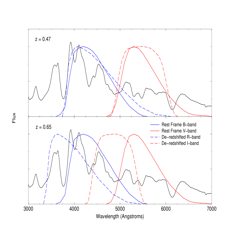
Figure 1: Filter pairings for $R$- and $I$-band observations of a redshifted SN Ia near maximum-light with respect to rest-frame $B$- and $V$-band filters. Nice matches occur at $z=0.47$ while large extrapolations occur at $z=0.65$.

In Hamuy et al. (1993) and Kim, Goobar and Perlmutter (1996) (hereafter H93 and KGP96) the $K$-corrections for samples of Type Ia supernovae (SNe Ia) were presented at both low- and high-redshift respectively. In H93 they dealt explicitly with the standard single filter $K$-corrections ($K_{BB}$ and $K_{VV}$). KGP96 developed the “cross-filter” $K$-corrections ($K_{BR}$ and $K_{VR}$) necessary for the determination of the cosmological parameters from high-redshift SNe Ia. Cross-filter $K$-corrections are necessary in the high-redshift searches since it allows one to work with the rest-frame optical light (where we have a good understanding of SNe Ia) and search photometrically where the observed light from a redshifted SN Ia is the brightest. Unlike the traditional single-filter $K$-correction only a small amount of extrapolation over a given spectrum is necessary. The only cost incurred by using cross-filter $K$-corrections is the small uncertainty in the zero points of the filter system. Figure 1 shows both an ideal case (at $z=0.47$) where the $B$- and $V$-band filters nicely match the de-redshifted $R$- and $I$-band filters (and the cross-filter $K$-corrections are insensitive to the underlying spectrum) and a less desirable one (at $z=0.65$) which involves some extrapolation or interpolation.

The dominant problem in applying $K$-corrections on real data is that one rarely has both photometric and spectroscopic observations of the same supernova at the same phase of its evolution. As a result, we are obligated to resort to existing libraries of supernova spectra from which we are to draw an appropriate $K$-correction for the photometric measurement in question. The spectra and time-series evolution of SNe Ia are remarkably homogeneous (Filippenko, 1997) but differences do exist (Nugent et al., 1995; Branch, Fisher & Nugent, 1993) which are undoubtedly linked to the variety of SN Ia light-curve shapes and possible foreground extinction.

The purpose of this paper is to further the work in KGP96 by synthesizing our current understanding of the spectra and light curves of SNe Ia to provide the best possible method for determining their $K$-corrections along with their associated errors. In particular we wish to focus on the effects that light-curve shape and reddening have on the $K$-corrections. One should note that the method presented here was developed and used for the analysis of the 42 high-redshift supernovae by the Supernova Cosmology Project (in Perlmutter et al. (1999), hereafter SCP99); it was also shared in advance of publication with the High-Z Supernova Search Team (HZSST) for their analysis of 14 additional high-redshift supernovae (Riess et al., 1998a) and it was briefly discussed in $\S~{}5$ of Gilliland, Nugent & Phillips (1999).

2 The Problem

The magnitude of a SN Ia in filter $y$ can be expressed as the sum of its absolute magnitude $M_{x}$, cross-filter $K$-correction $K_{xy}$, distance modulus $\mu$ and extinction due to dust in both the host galaxy, $A_{x}$, and our galaxy, $A_{y}$.

$$m_{y}(t(1+z))=M_{x}(t,s)+K_{xy}(z,t,s,A_{x},A_{x})$$

$$+\mu(z,\Omega_{M},\Omega_{\Lambda},H_{o})+A_{x}(t)+A_{y}(t).$$ (1)

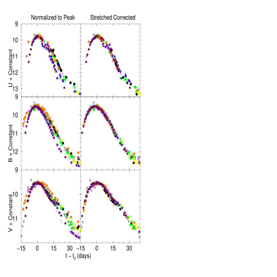
Figure 2: Left panels: The $UBV$-band light curves of several nearby SNe Ia adjusted to the same peak magnitude. Right panels: The same light curves corrected by their $B$-band stretch factor. Note the large reduction in scatter about the mean.

Here $t$ refers to the epoch when the SN Ia is being observed, $s$ is the stretch-factor [as described in Perlmutter et al. (1997), hereafter SCP97] and $z$ is the redshift. The stretch-factor, $s$, simultaneously parameterizes three aspects of the SN Ia light curve. First, it is responsible for changing the shape of the light curve. From an $s=1$ template, which is similar to the Leibundgut template for SNe Ia (Leibundgut, 1988), almost all known light curves for SNe Ia can be reproduced surprisingly well from the $U$-band through the $V$-band (over the time range $-20\lesssim t-t_{0}\lesssim+40$) by stretching the time axis of the light curve about maximum light by the factor $s$. This fact is highlighted in Figure 2 where we can see the large reduction in photometric scatter after the application of the stretch correction (see Goldhaber et al. (2001) for a quantitative study of this $B$-band stretch-factor fit). For the set of nearby supernovae in Figure 2 the peak-to-peak scatter for all photometric bands about a $s=1$ template decreases by a factor of 3 and 2 for +15 and +40 days after maximum light respectively after the stretch correction is applied to the data. Second, a relationship exists between the peak magnitude in $B$ for a SN Ia and $s$ that can be expressed as follows (SCP99):

$$M_{B}(t=0,s)=M_{B}(t=0,s=1)-\alpha*(s-1).$$ (2)

This is very similar to the relationship found by Phillips (1993) where a correlation between the peak brightness and the decline of the light curve from maximum light to +15 days ($\Delta$m${}_{15}(B)$) was presented. The broader light curves (smaller $\Delta$m${}_{15}(B)$) are intrinsically brighter, and the narrower light curves (larger $\Delta$m${}_{15}(B)$) are intrinsically fainter. Finally, there is a relationship between the color of SNe Ia and $s$ at peak $B$ brightness which can be expressed as follows:

$$B-V(t=0)=-\beta*(s-1)-\gamma.$$ (3)

This equation shows that the broader, brighter SNe are slightly bluer as well. (Note that the best fit values for the constants in Eqn’s 2 &  3 and their uncertainties can be found in SCP99. See also Phillips et al. (1999) for similar relationships with respect to $\Delta$m${}_{15}(B)$.)

The cross-filter $K$-corrections presented in this paper were calculated as they were in KGP96:

$$K_{xy}^{\rm counts}=-2.5\log\left(\frac{\int\lambda{\cal Z}(\lambda)S_{x}(\lambda)d\lambda}{\int\lambda{\cal Z}(\lambda)S_{y}(\lambda)d\lambda}\right)+2.5\log(1+z)$$

$$+2.5\log\left(\frac{\int\lambda F(\lambda)S_{x}(\lambda)d\lambda}{\int\lambda F(\lambda/(1+z))S_{y}(\lambda))d\lambda}\right).$$ (4)

Here $F(\lambda)$ is the spectral energy distribution (SED) at the source (in this case a supernova), $S_{x}(\lambda)$ and $S_{y}(\lambda)$ are the effective transmission of the $x$ and $y$-bands and ${\cal Z}(\lambda)$ is an idealized local stellar spectral energy distribution for which $U=B=V=R=I=0$ in the photometric system used here. $K_{xy}$ is defined as in Eq. 1. We have calculated the $K$-corrections as integrals of photon counts since here we have assumed a count-based photometric system. For a full description of why a count-based system is prefered see the appendix.

As can be seen in Eq. 1 the $K$-corrections are dependent on anything which affects the observed spectrum. This not only includes the obvious effects of redshift, $z$, and the spectral epoch, $t$, but the effects of stretch, $s$, and extinction, $A_{X}$ and $A_{Y}$, as well. As pointed out in Nugent et al. (1995) individual spectral features also vary slightly as a function of stretch in addition to the overall change in the broad slope of the SED mentioned above. Thus ideally what we need is a set of template SNe Ia spectra that cover a wide range in stretch, time and wavelength. Unfortunately at this time such a set of spectra is not available. However, as we will show, a very good approximation can be made that nicely accounts for almost all the spectroscopic differences among SNe Ia in order to accurately reproduce their $K$-corrections.

3 The Recipe

We would like to develop a simple yet effective method for determining $K$-corrections that encompasses the effects of stretch and extinction, overcomes gaps in existing spectroscopic data samples, and quantifies the uncertainties. H93 noted the following characteristic of the $K$-corrections for SNe Ia. “One of the most interesting features of this family of curves is their resemblance with the $B-V$ color curve of Ne Ia, implying that the $K$ term is basically driven by the color of the SN.” In Figure 3 we present the $K$-corrections for a typical, $s=1.0$, SN Ia at a variety of redshifts along with its $B-V$ color curve. The similarity of these curves is striking and for very good reason. It is the overall shape of the SED, i.e. the broad color differences rather than the individual spectral line features, which more than any other factor, determines the $K$-correction. In this paper we refer to these “overall SED colors” to describe the SED shape averaged over $\sim$1000Å bins.

Given this behavior we propose the following recipe for determining the $K$-corrections for a SN Ia.

1. Create a single template spectral grid of flux as a function of wavelength and time for a $s\approx 1.0$ SN Ia using all available “Branch Normal” SNe Ia (Branch, Fisher & Nugent, 1993).

2. Flux calibrate the spectra in the grid so that they yield as a function of time the standard relative magnitudes (in $UBVRIJHK$) of a $s=1.0$ SN Ia.

3. Adjust the overall SED colors for each time step of the grid to account for (a) extinction based on a given supernova’s measured $E_{B-V}$ and (b) the color differences as a function of the measured stretch factor of a given supernova. Both of these color adjustments are performed using a slope correction that follows the Cardelli et al. (1989) reddening law; as explained below, the stretch color differences have a very similar wavelength dependence.

4. For a given SN Ia measured properties ($s$, $z$, $E_{B-V}$) calculate the $K$-correction for each date, $t$, using integrals over the color-adjusted grid as in Eq. 4.

5. Propagate uncertainties in $s$, $z$, $E_{B-V}$, $t$ and in the constants of Eq 3 to estimate the $K$-correction uncertainties.

4 Testing the Method

Given the recipe outlined above we are now in a position to test the validity of calculating $K$-corrections from a single template of time evolving spectra, where the SED of any given spectrum can be altered to match the differences in stretch and/or extinction. Furthermore, we need to test the effects of interpolation in time between samples of observed spectra. While the database of SNe Ia has grown considerably in the past few years, there are very few spectra at a given epoch for a given supernova that go from the UV through IR. Additionally, for a given supernova, there are often large gaps in the spectral sequence, brought about by the supernova going behind the sun, a full moon or lack of continuing access to telescope time.

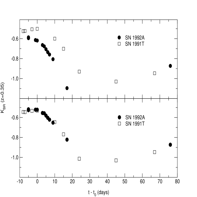
Figure 4: $K_{BR}$ at $z=0.35$ for SN 1992A (black circles) and SN 1991T (red squares). Top panel: $K$-corrections as would be observed for these spectroscopically distinct SNe Ia ($s=$ 0.80 and 1.09 respectively). Bottom panel: A slope correction was applied to each of the supernova’s spectra so that they would have the same $B-V$ colors as an $s=1.0$ SN Ia at every epoch.

We have made a couple of hypotheses here that we must test. Do different SNe Ia ($s$, $E(B-V)$) at the same epoch have the same $K$-correction after a color-adjustment on the overall SED color is applied (step 3 above)? We test this by examining the $K$-corrections for two very different SNe Ia 1992A and 1991T. The stretch values for these supernovae are nearly at opposite ends of the observed range, 0.80 and 1.09, and their reddening corrected $B-V$ colors at maximum light were -0.01 and -0.07 respectively (SN 1991T suffered from an extinction of $E(B-V)\approx 0.2$). In Figure 4a we see $K_{BR}$ at $z=0.35$ for both these supernovae and we note differences of at least 0.1 to 0.2 mag. over this time range. We chose this redshift, which involves a fair amount of extrapolation between the rest-frame $B$-band and de-redshifted $R$-band filters, to highlight the differences between the two SNe. In Figure 4b we have applied a slope correction to each of the supernova’s spectra so that they have the same $B-V$ colors as an $s=1.0$ SN Ia at every epoch. The slope correction was performed by altering the flux using the reddening law of Cardelli et al. (1989) (either making them bluer or redder accordingly). This is a reasonable approach since, while not exact, van den Bergh (1995), Riess et al. (1996) and Tripp & Branch (1999) have noticed that the intrinsic relationship between $M_{V}$ and $B-V$ for SNe Ia of varying stretch is quite similar to that of a typical dust reddening law. The result of these “color corrections” to the spectra is that the $K$-corrections now lie on top of each other with differences between the curves of at most 0.02 mag. It is well known that these particular supernovae show several differences spectroscopically (e.g. see Nugent et al. (1995) and Branch, Fisher & Nugent (1993)), however, for the $K$-corrections these differences are quite small compared to the effect of the overall SED colors.

We do note the following exception to this method. SN 1991bg, a peculiar, sub-luminous SN Ia (with $s<0.7$), has a large trough in its spectra due to several strong Ti II spectral lines (Filippenko et al., 1992). This feature is over 400Å wide and persists quite strongly for several months. The color difference between a $s=1.0$ SN Ia and a 91bg-like supernovae at maximum light is $>0.8$ in $B-V$, and is due almost completely to the presence of these Ti II lines. The “color correction” method mentioned above will not work with these types of SNe Ia. Instead, one would have to create a set of template spectra based solely on 91bg-like supernovae.

How well do the temporal interpolations work? Since we see that it is the overall SED colors which are the largest factors in the $K$-correction, and not individual spectral features, we have some confidence in interpolating between different supernovae across a wide range of epochs. A test of this method is seen in Figure 5. Here we once again display $K_{BR}$ for a $z=0.35$ SN Ia with $s=1.0$ along with three other sets of $K$-corrections, chosen to mimic the effect of mis-identifying the date of a spectrum or poorly interpolating between dates. These $K$-corrections were calculated by forcing the spectra within 10 days of a given point on the light curve to have the same colors as the SN Ia has at that central point. This was done for maximum light, $+10$ days and $+20$ days. The difference in the $K$-corrections is, at most, 0.05 mag over the entire 20 day window and $\lesssim$ 0.02 mag. for a 10 day window. Thus the spectral feature evolution of a SN Ia has a negligible contribution to the change in the $K$-correction over periods of roughly one week compared to the changes in the overall SED colors. This also gives us confidence in interpolating between spectra of slightly separated epochs, so long as the overall SED colors are correct.

5 SN Ia Template

Table $K$-corrections and Extinction Corrections for Type Ia Supernovae lists the SNe Ia used to construct the template. In Table 2 we list the $UBVRIJHK$ magnitudes used to determine the overall SED colors for this $s=1.0$ SN Ia template. Note that this is a preliminary template and will certainly change in the future as more and better observations of SNe Ia are obtained. The preliminary nature of this template has no effect on the results presented in this paper, since our goal here is to stress the method rather than the actual values for the $K$-corrections. The color template was created from four primary sources. The $B$- and $V$-band light curves come from the data of Riess et al. (1999a) and the $R$, $I$ light curves from Knop (2002) (see also Goldhaber et al. (2001) for comparable $B$-band templates). . The $JHK$ photometry comes from the work of Elias et al. (1981) and the $U$-band data from the work in Branch et al. (1997). The early, rising, portion of the light curve, which is well mapped out in $B$ and $V$ prior to -10 days, was extrapolated in all other filters in a smooth way such that the explosion date for this SN Ia occurs 20 days before maximum light in $B$.

The set of observed spectra was assembled in a two dimensional grid of flux as a function of time (1 day bins with $-19<t<70$) and wavelength (10 Å bins with 2500 Å $<\lambda<$ 25000 Å). If two or more spectra on a given day overlapped we used their noise-weighted average. All the spectra were then “color corrected” by the method outlined above to have the colors listed in Table 2. To fill in the temporal gaps, a simple linear interpolation was applied throughout the set. Extrapolation was only used prior to day $-14$ and just for the UV after day $+45$. The entire set was then smoothed in a given wavelength bin, using a gaussian-weighted boxcar approach, over time (a $\sigma$ = 2 days was used). This removed any “glitches” (such as poor cosmic-ray subtractions, etc.) from the overall template. Finally a last “color correction” was applied to this grid of spectra. In Figure 6 we present a sampling of the template from two weeks before to four weeks after maximum light.

6 Error Budget

We now turn our attention to the error associated with making a given $K$-correction. We have already considered the first component of this error in § 4. This is the error incurred when using the template method and is a result of the effectiveness of the “color correction” across the SN Ia sub-type and the interpolation in time of the spectra. In the worst-case-scenario for rest-frame optical cross-filter $K$-corrections ($z\approx 0.35$) there is $<$ 1% rms dispersion over the entire light curve due to differences in supernova sub-type, and $<$ 1% dispersion due to interpolations in time of the spectra, when constrained to $\pm$ 4 days.

The second component of the error is purely observational and depends on two factors: (1) the alignment of the de-redshifted filter (on which the $K$-correction will be performed) with respect to the rest-frame filter and (2) the photometric error on the observed color of the supernova. This overall observational error vanishes for either perfectly matched filters or zero error in the color measurement.

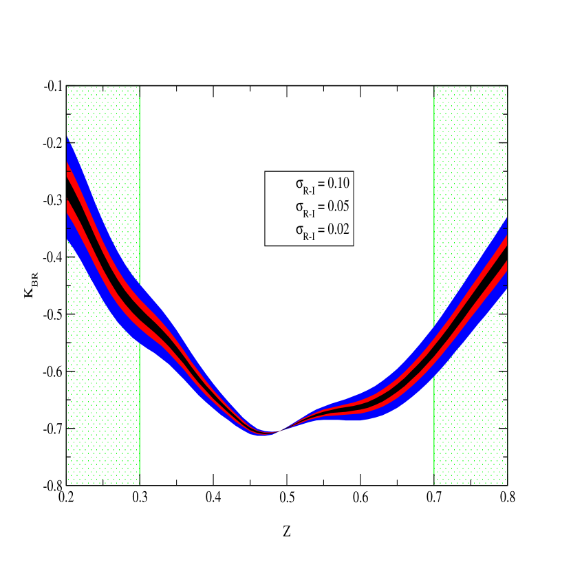
Figure 7: $K_{BR}$ as a function of $z$ for three different cases in which we assign an uncertainty in the observed $R-I$ color of 0.02 (black), 0.05 (red) and 0.10 (blue). Note how the uncertainty in $K_{BR}$ vanishes at $z=0.49$, where the rest-frame $B$ and de-redshifted $R$-band filters nicely overlap, regardless of the uncertainty in the color measurement. In practice one does not use $K_{BR}$ in the green regions, where a switch is made to a more appropriate filter.

To illustrate this error we present in Figure 7 $K_{BR}$ as a function of $z$. Here we have calculated this $K$-correction for three different cases in which we assign an uncertainty in $R-I$ of 0.02, 0.05 and 0.10. The most striking fact about this graph is how the uncertainty in $K_{BR}$ vanishes at $z=0.49$, where the rest-frame $B$ and de-redshifted $R$-band filters nicely overlap, regardless of the uncertainty in the color measurement. One also notices how the uncertainty in the $K$-correction flares out at the upper and lower ranges in redshift. In practice, when trying to obtain rest-frame corrected $B$-band photometry, $K_{BR}$ is not used for SNe Ia with $z\lesssim 0.3$ or $z\gtrsim 0.7$. A switch is made to $K_{BV}$ or $K_{BI}$, respectively, to perform the $K$-correction. At these redshifts, where the rest-frame $B$ and de-redshifted $R$-band filters barely overlap, the uncertainty in the observed color of the supernova translates directly into a larger uncertainty in the $K$-correction. For example, at $z=0.3$ we note that $\sigma_{K_{BR}}\approx\sigma_{B-V}$. While this may seem like it would impart a large uncertainty in the corrected $B$-band magnitude it is in fact dwarfed by the error in the extinction correction. Given that $A_{B}=4.1E(B-V)$ we see the fact that $\sigma_{A_{B}}$ is a factor of four larger than the $\sigma_{K_{BR}}$. Thus the major problem facing individual high-redshift SN Ia photometry will always lie in the accuracy of multi-color photometry, not in performing $K$-corrections.

6.1 Problems with Restframe $U$-band Photometry

As automated searches for supernovae continue to progress, one of the greatest problems faced in the reduction of this data concerns our knowledge of the rest-frame UV light. Many problems exist with current $U$-band photometry from an observational standpoint alone (Richmond et al., 1995). When this is coupled with the large intrinsic variations among similar SNe Ia in the UV (Branch et al., 1997) and the larger uncertainties in absolute UV photometry due to extinction, one can easily see that that working in this area of the spectrum is problematic at best. Here we provide two examples of how the above stated problems affect our current understanding of SNe Ia.

The highest redshift SNe Ia that have been confirmed spectroscopically are SN 1998eq (Aldering et al., 1998) at a $z=1.20$ and SN 1999fv (Coil et al., 2000) at a $z=1.19\pm 0.02$. Both supernovae were discovered in the $I$-band. The SCP was able to follow SN 1998eq in the $J$-band with NICMOS on board the HST while the HZSST obtained a deep image of SN 1999fv in the $J$-band from the ground (Tonry, 2000). Both teams will rely on the $I$-band photometry of the supernovae to determine the shape of its light curve (the $I$-band maps almost directly with the rest-frame $U$-band at these redshifts) and use the $J$-band photometry to infer the peak rest-frame $B$-band magnitude. However, current uncertainties in the intrinsic $U-B$ colors of SNe Ia are quite large. A $s=1.0$ SNe Ia has $\sigma_{U-B}\geq 0.1$ which implies an uncertainty in $A_{B}\geq 0.5$ ($A_{B}=4.8E_{U-B}$) (Branch et al., 1997; Perlmutter et al., 1998). Without any other constraints on the total reddening these supernovae become quite ineffective in discriminating between various cosmological models.

Not only does our current understanding of the UV affect our interpretation of the very high-redshift SNe Ia, but it affects our knowledge of nearby supernova and therefore our current understanding of the relationship between light-curve shape and peak brightness as well. In Table 3 we present the differences between SN 1992A and SN 1994D in their rest-frame $U-B$ and $B-V$ colors and in $K_{BB}$ if these SNe Ia were found at a redshift of $z=0.1$. These two SNe Ia have very similar stretches ($s\approx 0.81$) but very different colors in the blue as is seen quite clearly in Figure 4 of Patat et al. (1996). Table 3 highlights how these differences lead to very different $K$-corrections as a function of time. Depending on the sampling, a SN Ia observed at this redshift whose $K$-correction did not account for color differences in the UV could yield reduced $B$-band light-curve shapes which are incorrect by $>$10%. This difference would create a 0.17 magnitude offset in the distance modulus (see Eq. 2). SNe Ia at this redshift are particularly important for the Hubble diagram since they are well out in the Hubble flow and thus unaffected by host galaxy peculiar velocities. One possible explanation of the difference in the UV color can be found in the work of Höflich et al. (1998) where the metallicity of the progenitor can have a strong influence on the UV spectrum. Lentz et al. (2000) has quantified these effects by varying the metallicity in the unburned layers and computing their resultant spectra at maximum light with the spectrum synthesis code PHOENIX (Nugent et al., 1997; Nugent, 1997). The differences seen in the theoretical calculations easily span the range seen between SNe 1994D and 1992A and are quite plausible as an explanation for the large intrinsic scatter in the UV for SNe Ia given the range in progenitor environments for these objects (Hamuy et al., 2000).

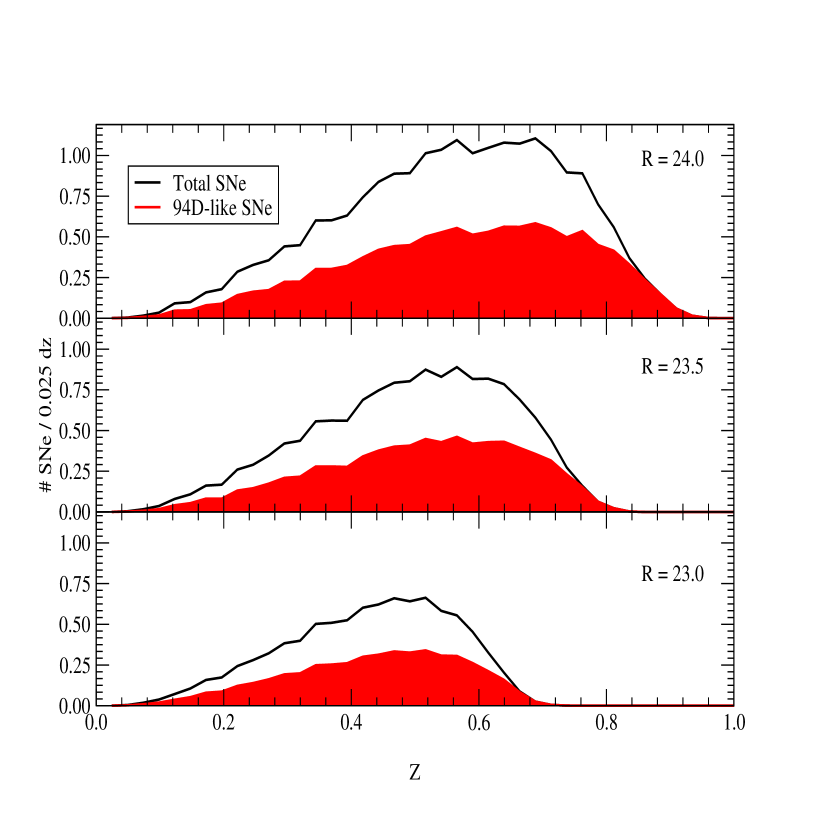
Figure 8: An $R$-band Monte Carlo search for SNe Ia covering a one month gap between reference and discovery and 4 square degrees on the sky given an equal distribution between the blue SN 1994D-like supernovae and the red SN 1992A-like supernovae. The solid black line plots the total number of supernovae discovered per 0.025 $dz$ while the filled red area shows the total fraction which are 1994D-like. The bias becomes apparent at $z>0.5$.

We conclude this section with a final note on how the intrinsic differences in the $U$-band photometry can affect a bias on the high-redshift search for SNe Ia. Given the differences seen in the $U-B$ colors for the two SNe Ia above, we can perform a simple Monte-Carlo search for supernovae along the lines of Gilliland, Nugent & Phillips (1999), to estimate the likelihood of finding the bluer SN 1994D’s over the redder SN 1992A’s. In Figures 8, 9 and 10 we have plotted the discovery rate for a search with a 50-50 split between supernovae like 1994D and those like 1992A. In the $R$-band search we have modeled the Monte Carlo after a typical 4-m telescope run like those carried out by the SCP (SCP99) and HZSST (Riess et al., 1998a) between 1995 and 1998. The search covers 4 square degrees with a 28 day separation between the reference and discovery images and has limiting magnitudes, typical for those searches, of 23.0, 23.5 and 24.0. What is clearly seen from the figures is the strong bias above a redshift of 0.5 (where the restframe $U$-band light slips into the $R$-band filter) for discovering blue SNe Ia. Of the SNe Ia presented in the aforementioned papers over 33% are at $z>0.5$ and thus susceptible to this bias. More recently the searches conducted by both teams have been carried out in the $I$-band with the goal of discovering even higher redshift supernovae. For this Monte Carlo we assumed a search gap of 28 days and 1 square degree to limiting magnitudes of 24.0, 24.5 and 25.0. Going to the redder filter we see the bias affecting the search for $z>0.9$.

How would such an effect alter the measurement of the cosmological parameters? First one would have to know the relative rates of 94D-like to 92A-like supernovae at any given redshift which is completely uncertain at the moment. However, even assuming an equal distribution of the rate of both populations, on face value there would be little difference. Both SN 1992A and SN 1994D appear to have similar absolute peak brightnesses in the restframe $B$-band given the intrinsic uncertainties in the SN Ia calibration and the distances to their host galaxies (Ajhar et al., 2001). The major difference would lie in color corrections based on the uncertainties in the $K$-corrections for those supernovae at redshifts where the restframe $U$-band light contaminates the correction to the $B$-band measurement. Given a split distribution and the Monte Carlo simulations above we would expect to find, on average, bluer supernovae at higher redshift and potentially underestimate the correction due to host galaxy extinction. This would lead one to overestimate distances to these objects.

However, in general, this effect is quite limited. This is due to the fact that the total amount of reddening a supernovae can have which is discovered near the edge of detection is quite small. This is further amplified by the fact that since one is looking at the rest-frame UV light, which suffers a higher relative extinction, even less reddening is allowed before the supernova becomes too extinguished to discover. Even for those 94D-like supernovae with a small amount of extinction that still get discovered, the effect of under-correcting for extinction, and thus overestimating the distance to those supernovae, is compensated by the fact that these supernovae are brighter in the UV and the flux in the observed filter is higher than average.

In practice, as was reported in Knop (2002), one can use both the 94D-like templates and the 92A-like templates to compute the $K$-corrections for the high redshift supernovae. The differences in the overall fits to the cosmological parameters are quite small, though one definitely produces systematic differences in the color distributions of the high-redshift supernovae based on the choice of template. The simple solution to this problem is to observe the high-redshift SNe Ia farther into the red where the restframe $U$-band light does not play a significant role in determining the corrected $B$-band magnitude.

6.2 Problems with Restframe $I$-band Photometry

One of the interesting characteristics of SNe Ia is the shape of the light curves in the near IR. In the $I$-band there exists a secondary peak which occurs more strongly, and at a slightly later epoch, for the more luminous supernovae while less luminous SNe Ia like SN 1991bg hardly show this secondary peak at all (e.g. see Hamuy et al. (1996); Riess et al. (1999b); Krisciunas et al. (2001)). This feature in the $I$-band light curves is in part due to the presence of the strong emission from the Ca II IR triplet. The emission is delayed in the brighter supernovae and is much stronger when it peaks compared to the fainter supernovae.

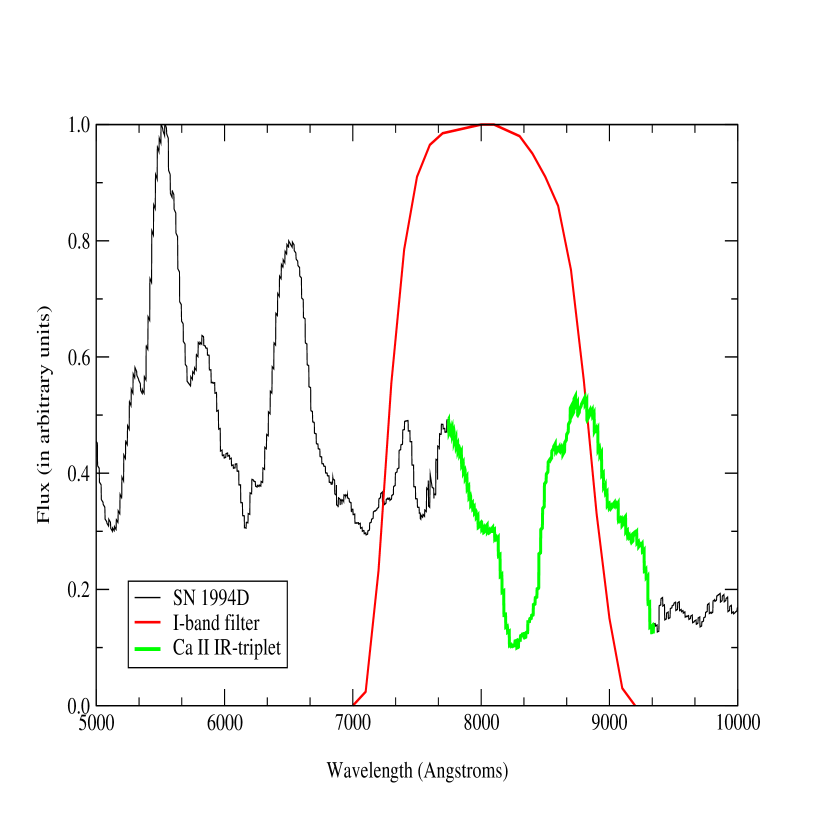
Figure 11: SN 1994D (in black) at 24 days after maximum $B$-band light (Patat et al., 1996). Highlighted are the strong Ca II IR triplet feature (in green) and the Bessel $I$-band filter function (in red). Errors in the $K$-corrections can be quite significant, even at low redshift, if one does not compensate for the change in the feature’s strength with epoch and luminosity class.

In the restframe, the $I$-band straddles this P-Cygni profile which is almost 1000 Å wide as seen in Figure 11. Even for low-$z$ supernovae this feature poses a problem. At a redshift of just a few percent ($z\approx 0.05$) the $I$-band filter moves completely off the emission feature. Thus $K$-corrections which are based on the template method outlined above which can not compensate for the change in this feature’s strength due to epoch and luminosity-class can be in significant error. In Strolger et al. (2002) differences approaching 0.3 magnitudes were seen using various template methods compared to using the actual supernovae spectra to perform the $K$-correction. Clearly the solution to this problem is to derive separate templates based on luminosity class for performing the $K$-corrections. This is exactly the same type of problem mentioned before in the $B$-band for the low-luminosity SNe Ia due to the presence of the Ti II trough.

7 Reddening

We now turn our attention to the effects of reddening on the light curves of SNe Ia. There are two factors we must consider here. First, as pointed out by KGP96, the observed color excess of a SN Ia will vary slightly with time because the rapidly varying SED shifts the effective wavelength of each filter. Second, Phillips et al. (1999) (hereafter P99) have noted that the observed decline rate of a SN Ia is a weak function of the dust extinction which affects the light curves. Both of these effects directly impact one’s ability to accurately measure the light-curve shape and peak corrected-magnitude of a SN Ia.

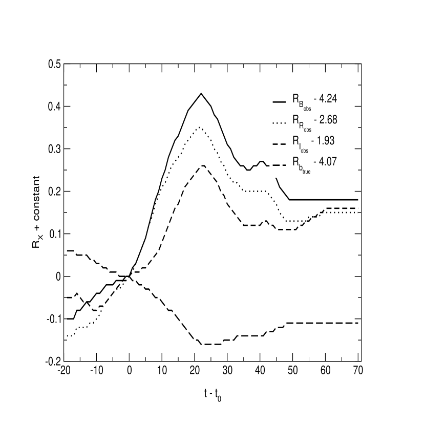
Figure 12: The relative variations of $R_{X}=A_{X}/E(B-V)$ as a function of time. The calculations were performed for $B$, $R$ and $I$ ($V=R_{B}-1.0$ by definition and thus is not shown). Both $R_{B_{obs}}$ and $R_{B_{true}}$ are displayed. Each serves a purpose for performing color corrections depending on whether one wants to correct photometry based on their observed colors, or if one a priori knows $E(B-V)_{true}$ along the line of sight to the SN Ia in question.

We start with a few definitions. $E(B-V)_{true}$ is a measure of the absorbing gas and dust along the line of sight to the supernova, not the observed color excess, $E(B-V)_{obs}$, which will vary with supernova epoch and total extinction. In Figure 12 we have plotted the relative variations of

$$R_{X}=A_{X}/E(B-V)$$ (5)

as a function of time. The calculations were performed for $B$, $R$ and $I$ ($V=R_{B}-1.0$ by definition and thus is not shown) using the spectral template of § 5. We display both $R_{B_{obs}}$ and $R_{B_{true}}$. Each serves a purpose for performing color corrections depending on whether one wants to correct photometry based on their observed colors, or if one a priori knows $E(B-V)_{true}$ along the line of sight to the SN Ia in question. Over the first 40 days of the light curve $R_{B}$ is found to vary considerably, $-0.1\lesssim R_{B}\lesssim 0.4$. The variation is caused by the rapid evolution in the spectra of SNe Ia around maximum light noted by the change in $\lambda_{eff}$ as mentioned above.

P99 found the following relationship between the true decline rate and the observed decline rate as a function of $E(B-V)_{true}$.

$$\mbox{$\Delta$m${}_{15}(B)$}_{true}\simeq\mbox{$\Delta$m${}_{15}(B)$}_{obs}+0.1E(B-V)_{true}$$ (6)

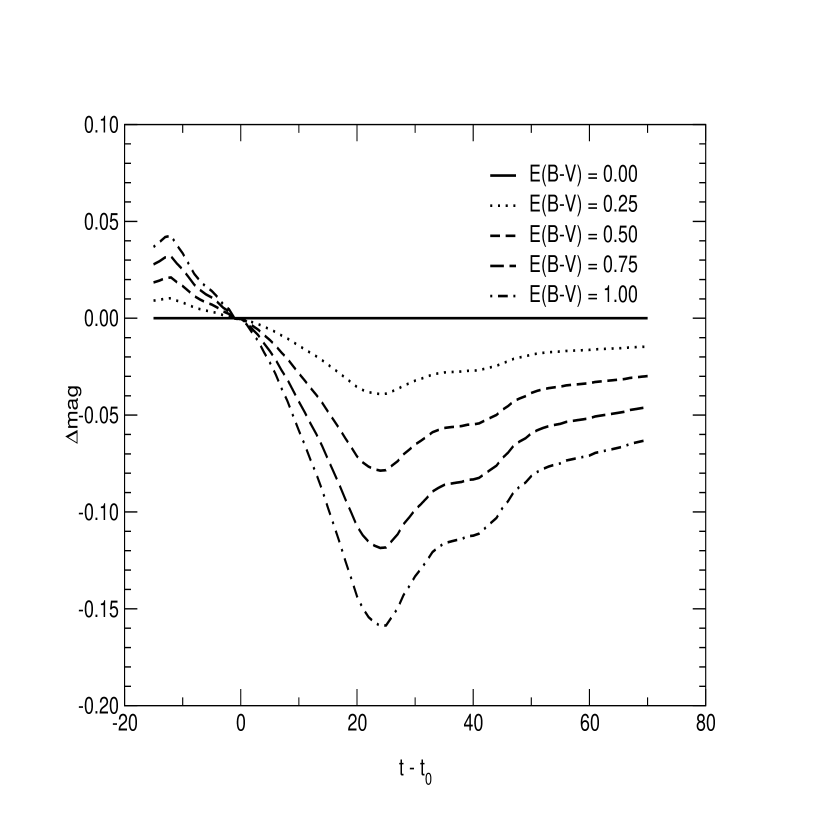
Figure 13: The relative difference in $B$-band magnitude (normalized at maximum light) between an unextinguished light curve and several increasingly extinguished light curves.

This shows that from peak to +15 days the light curves of SNe Ia get broader as they become more extinguished by dust. In Figure 13 we plot the relative difference in $B$-band magnitude (normalized at maximum light) between an unextinguished light curve and several increasingly extinguished light curves. These curves were calculated using the spectral template from § 5 and the same reddening law employed by P99 (Cardelli et al., 1989). Here one can clearly see the result found by P99, however, the pre-maximum portion of the light curve does not behave in a similar way. Our results show that extinguished light curves are narrower prior to maximum light and broader past maximum light. The explanation for this result is quite simple. For a given epoch, a reddened spectrum produces a shift in the effective wavelength, $\lambda_{eff}$, of the spectrum, $F(\lambda)$, integrated through the filter, $S(\lambda)$, toward the red. $\lambda_{eff}$ is given by the following equation:

$$\lambda_{eff}=\frac{\int\lambda F(\lambda)S(\lambda)d\lambda}{\int F(\lambda)S(\lambda)d\lambda}.$$ (7)

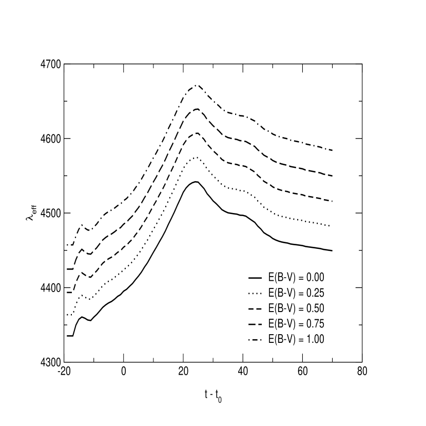
Figure 14: $\lambda_{eff}$ as a function of time for various levels of extinction in the $B$-band. Note that for a given amount of extinction a supernova naturally becomes cooler and redder as a function of time in addition to the expected shift in the effective wavelength as a function of extinction.

In Figure 14 we have plotted $\lambda_{eff}$ as a function of time for various levels of extinction in the $B$-band. We note that a supernova naturally becomes cooler and redder as a function of time after maximum light and for a given amount of extinction there is also the expected shift in the effective wavelength. Thus a simple minded explanation for the change in a heavily reddened SN Ia’s $B$-band light curve is that the shift in effective wavelength makes the light curve act more like a $V$-band light curve, which is broader after maximum light but narrower prior to it (see Table 2). Therefore, it would be incorrect to interpret the equation in P99 as something which is applied to a given $\Delta$m${}_{15}(B)$light-curve class. Rather it should only be used in the strict interpretation of $\Delta$m${}_{15}(B)$, the change in magnitude from peak to +15 days.

8 Examples of Extinction and $K$-correctionson Observed Data

In this section we look at the application of the template method with regards to both reddening corrections on three nearby SNe Ia and $K$-corrections on one of the SCP’s first set of seven high-redshift supernovae.

8.1 SNe 1998bu, 1986G and 1996ai

SNe 1998bu (Suntzeff et al., 1999; Jha et al., 1999), 1986G (Phillips et al., 1987) and 1996ai (Riess et al., 1999b) were three well observed SNe Ia caught prior to maximum light and followed regularly for over two months in multiple filters. All three suffered from a large amount of extinction: SN 1998bu had $E(B-V)\approx 0.37$, SN 1986G had $E(B-V)\approx 0.6$ and SN 1996ai had $E(B-V)\approx 1.68$.

As outlined in the previous section, the biggest effect that the reddening has on a SN Ia (outside of the obvious color change) is its ability to alter the observed stretch of the light curve. For these three SNe the $B$-band stretch should be decreased from the observed values by the following amounts: SN 1998bu – 3%, SN 1986G – 5% and SN 1996ai – 11%. Eq. 2 implies that without performing the aforementioned correction to the stretch due to the extinction along the line of sight to the supernovae their distance moduli would be overestimated by 0.05, 0.09 and 0.19 mag respectively.

A secondary effect one needs to consider is that a given stretch implies a particular $B-V$ color evolution for the supernova. If one used the peak observed $B-V$ color of these supernovae coupled with their observed $B$-band stretch they would falsely arrive at a higher value of $E_{B-V}$ for each. This is simply due to the fact that the observed $B$-band stretch of an extinguished SN Ia is broader than its true, intrinsic stretch and a narrower stretch SN Ia is redder than a broader one. Therefore using the stretch corrections to the extinguished SNe above coupled with Eq. 3 we see that the true value of $A_{B}$ would be altered by the following amounts: SN 1998bu – 0.02, SN 1986G – 0.04 and SN 1996ai – 0.09 mag. This goes in the opposite direction of the corrections outlined above and thus slightly mitigates the overall effect that reddening has on the distance determinations to SNe Ia. However ignoring this effect increases the overall dispersion in the stretch luminosity relationship.

8.2 SN 1994H

As seen in SCP99, SN 1994H (one of the first seven supernovae published in SCP97) was one of two large outliers in the Hubble diagram of the SCP’s high-redshift SNe Ia. It was also one of the few supernovae without a spectrum to confirm its classification and it was excluded from all of the primary fits of SCP99. Using a brute-force multi-dimensional $\chi^{2}$ fitting program which incorporates the template in § 5, we have calculated the best fit to the light curve of this supernova (a modified version of this method was used in SCP99. From this we find the best fit stretch to be $s=0.90\pm 0.06$. The supernova had an observed color which was bluer than $B-R=0.7$ at 0.0$\pm$0.6 days at the 95% confidence limit. A SN Ia at this redshift ($z=0.374$) and stretch will have an unextinguished $B-R$ color of 1.63$\pm$0.05 (the error bars are the result of the uncertainties in the time of maximum light and stretch). The difference between the observed color and the one calculated for a SN Ia of this stretch are many standard deviations apart. Reddening, of course, only makes this supernova more discrepant.

This result, seen in SCP99, differs from the result first presented in SCP97 due to the fact that the fitting procedure used at that time did not vary the $K$-corrections as a function of stretch. At this redshift, where the extrapolation is large, these differences are considerable. For SCP97 the stretch was determined to be 1.09$\pm$0.05, which would place this supernova in the very broad–bright–blue category of SN Ia along the lines of SN 1991T(Phillips et al., 1992). The $B-R$ color of a SN 1991T-like supernova at this redshift is $B-R\approx 1.0\pm 0.15$, which, as pointed out in SCP97, is only in mild disagreement with the observed color..

The implication of this result is that SN 1994H was most likely a Type IIL or II-n supernova caught at an early phase. Given that most SNe II look like blackbodies early in their light curves, the $B-R$ color of 0.7 mag is not too surprising. In fact, the color at this redshift implies a blackbody temperature of 9750 ^∘K, which is quite consistent with a SN II at this phase. Given a cosmology of $h=0.635$, $\Omega_{M}=0.3$ and $\Omega_{\Lambda}=0.7$ with a $K_{BR}=-0.68$ for a 9750 ^∘K blackbody, we find that SN 1994H would have an $M_{B}\gtrapprox-19.60$. This would make it a rather luminous SN II along the lines of SN 1979C (Branch et al., 1981; de Vaucouleurs et al., 1981). This result strengthens the case for the primary cosmology fit of SCP99 which excluded SN 1994H.

9 Conclusions

We have presented a method for performing generalized $K$-corrections for SNe Ia which allows us to compare these objects from the UV to near-IR over the redshift range $0.0<z<2.0$ along with the corresponding uncertainties currently associated with this method. These uncertainties are in general much smaller when compared to the uncertainties in the extinction corrections. Future data will certainly improve upon this method considerably, especially if properly calibrated spectral templates can be acquired for each sub-class of SNe Ia. We have also examined the effects of reddening on the light curves of nearby SNe Ia and how our current, poor understanding of the behavior of SNe Ia in the UV effect the use of SNe Ia at both high- and low-redshift.

APPENDIX

Appendix A Photon versus Energy K-corrections

Measurements of the cosmological parameters using distance indicators rely on the redshift-dependent evolution of the distance modulus $\mu$. The distance modulus is measured as the difference between observed and absolute magnitudes of a “standard candle” after $K$-correction (Oke & Sandage, 1968) for the redshifting of its spectrum. The theoretical value for $\mu$ is related to the luminosity distance $d_{L}(z)$ defined such that a source with luminosity $L$ at redshift $z$ has observed energy flux $f$ as if the energy has been diluted to the surface of a sphere with radius $d_{L}$, i.e. $L=4\pi d_{L}^{2}f$ (e.g. Carroll et al. (1992)). Cosmological parameters can then be measured from their functional dependence on $d_{L}$.

Observations are in fact made with photon counters (CCD’s, photo-multipliers) and the luminosity distance is not the same as the “photon luminosity distance” $d_{\gamma}$; if N is the photon luminosity and n is the observed photon flux, then $N=4\pi d_{\gamma}^{2}n$ where $d_{L}=d_{\gamma}(1+z)^{1/2}$. This has lead to some confusion as to whether a “photon” distance modulus should be used to measure cosmological parameters, whether the magnitude system is photon-based or energy-based, and which $K$-corrections should be applied. Such distinctions which previously have been unimportant are significant as we move into an era of precision cosmology. In this appendix we rederive and expand upon the $K$-correction results of Schneider et al. (1983). We comment on the magnitude system and the Johnson-Cousins system in particular (§ A.1). We find that any ambiguity can be removed with the proper definition of the $K$-correction for which we derive the equations for both photon and energy systems (§ A.2). We conclude that although the differences between the two $K$-corrections are small, the distinction between energy and photon systems is important for planned future high-precision supernova experiments (§ A.3).

A.1 Magnitude Systems

The primary standards of a photometric system can have their magnitudes measured either by their energy or photon flux ratios. Unless a photon–energy conversion correction is later applied, the flux system is determined by the detectors used to measure the primaries. The type of detector used in subsequent observations does not determine whether the magnitude system is photon or energy based; in principle the color and airmass corrections put observed magnitudes into the primary system.

The Johnson-Cousins magnitude system prevalent today is a photon system, what Johnson & Morgan (1953) describe as “a system of photoelectric photometry”. As described in Johnson & Morgan (1951), their observational setup employed a photomultiplier as a detector, with the counts being the number of “deflections” recorded by a potentiometer. After an airmass correction these counts were directly converted to magnitudes. The secondary stars of Landolt (1973, 1983, 1992) (whose raw data also were obtained with photon counters) are calibrated via Johnson and Cousins primary standards and thus must be in the photon system. Observed magnitudes are therefore photon-based and should be analyzed as such.

An illustrative example of where there is a numerical difference between the two magnitude systems is a star that has the same integrated $B$-band energy flux as Vega (which for simplicity we consider to be the zero point of the magnitude system) but has a different photon flux since it has a different spectral energy distribution (SED). Relative magnitude measurements with a single filter of a set of stars with similar spectral energy distributions are independent of whether we are photon counting or measuring energy; two stars with the same SED but differing brightness will have

$$\Delta m=m_{2}^{\gamma}-m_{1}^{\gamma}=m_{2}^{\epsilon}-m_{1}^{\epsilon}$$

where $m_{1}$ and $m_{2}$ are the stars’ magnitudes. It follows that since the zeropoint of magnitude system is based on Vega, the energy and photon magnitudes of A0V stars are identical: $m_{A0V}^{\gamma}=m_{A0V}^{\epsilon}$.

As an aside, one of the Johnson & Morgan (1953) criteria for a photometric system is “a determination of the zero point of the color indices in terms of a certain kind of star which can be accurately defined spectroscopically.” Such knowledge, along with the shapes of the pass-band transmission functions, do allow for calculated transformation between photon and energy magnitude systems. Indeed, much effort has been placed in measuring and modeling the intrinsic SED of Vega (Dreiling & Bell (1980) and references therein).

A.2 The $K$-correction

We explicitly review the $K$-correction calculation of Kim et al. (1996) that has been used in SCP cosmological analysis. To remove any ambiguity we define the $K$-correction $K_{xy}$ such that

$$m_{y}^{\alpha}=M_{x}^{\alpha}+\mu(z)+K_{xy}^{\alpha}$$ (A1)

where $\alpha=\{\gamma,\epsilon\}$ for photon or energy magnitude systems. The observed magnitude in passband $y$ is $m_{y}$ and the absolute magnitude in passband $x$ is $M_{x}$. We adopt the theoretical expression for the distance modulus, $\mu$, based on luminosity distance. In other words, the functional form of $\mu(z;H_{0},\Omega_{M},\Omega_{\Lambda})$ in Equation A1 is identical for photon and energy systems. Given $f_{\lambda}(\lambda)$ as the energy flux density of a supernova 10 parsecs away, we can compute the corresponding energy and photon fluxes at high redshift.

$$\begin{array}[]{lr}f_{\lambda}(\lambda)d\lambda&\mbox{Energy flux density in d$\lambda$ bin of a supernova 10 parsecs away}\\ n_{\lambda}(\lambda)d\lambda=\frac{\lambda d\lambda}{hc}f_{\lambda}(\lambda)&\mbox{Photon flux in d$\lambda$ bin of a supernova 10 parsecs away}\\ f^{z}_{\lambda}(\lambda)d\lambda=\frac{d\lambda}{1+z}f_{\lambda}\left(\frac{\lambda}{1+z}\right)\left(\frac{10pc}{d_{L}(z)}\right)^{2}&\mbox{Energy flux density in d$\lambda$ bin of a supernova at $z$}\\ n^{z}_{\lambda}(\lambda)d\lambda=\frac{\lambda d\lambda}{hc(1+z)}f_{\lambda}\left(\frac{\lambda}{1+z}\right)\left(\frac{10pc}{d_{L}(z)}\right)^{2}&\mbox{Photon flux density in d$\lambda$ bin of a supernova at $z$}\end{array}$$

The $(1+z)^{-1}$ terms in the redshifted flux densities are due to wavelength dilution (Oke & Sandage, 1968). The ratio between high and low-redshift photon flux is a factor $1+z$ greater than the corresponding ratio for energy flux which suffers from redshifted energy loss. More precisely

$$\frac{n^{z}_{\lambda}(\lambda)}{n_{\lambda}(\lambda/(1+z))}=\frac{(1+z)f^{z}_{\lambda}(\lambda)}{f_{\lambda}(\lambda/(1+z))}.$$ (A2)

The fact that the relative photon fluxes of high-redshift supernovae are $1+z$ “brighter” than energy fluxes can be interpreted as being due to the latter’s extra energy loss due to redshift.

Using the fact that $\mu=-5\log{\left(\frac{10pc}{d_{L}(z)}\right)}$ we can compute and compare energy and photon $K$-corrections,

$$K_{xy}^{\epsilon} = -2.5\log\left(\frac{\int{\cal Z}^{\epsilon}_{x}(\lambda)S_{x}(\lambda)d\lambda}{\int{\cal Z}^{\epsilon}_{y}(\lambda)S_{y}(\lambda)d\lambda}\right)+2.5\log(1+z)+2.5\log\left(\frac{\int f_{\lambda}(\lambda)S_{x}(\lambda)d\lambda}{\int f_{\lambda}(\lambda/(1+z))S_{y}(\lambda)d\lambda}\right)$$ (A3)

$$K_{xy}^{\gamma} = -2.5\log\left(\frac{\int\lambda{\cal Z}^{\gamma}_{x}(\lambda)S_{x}(\lambda)d\lambda}{\int\lambda{\cal Z}^{\gamma}_{y}(\lambda)S_{y}(\lambda)d\lambda}\right)+2.5\log(1+z)+2.5\log\left(\frac{\int\lambda f_{\lambda}(\lambda)S_{x}(\lambda)d\lambda}{\int\lambda f_{\lambda}(\lambda/(1+z))S_{y}(\lambda)d\lambda}\right).$$ (A4)

The filter transmission functions are given as $S_{i}(\lambda)$ where $S_{x}$ is the rest-frame filter and $S_{y}$ is the observer filter. (The transmission functions give the fraction of photons transmitted at a given wavelength where we assume no down-scattering.) For the standard star (i.e. calibrator) SED ${\cal Z}(\lambda)$ we assume the existence of a standard star with identical properties as the supernova, i.e. with exactly the same color and observed through the same airmass. Pragmatically, this assumption affirms perfect photometric calibration to all orders of color and airmass. For convenience, we choose these secondary standards to have 0 magnitude. In principle, a different standard will be needed for each filter, choice of photon or energy flux, and each source SED. Each standard is labeled ${\cal Z}_{X}^{\alpha}$ where $X=\{U,B,V,R,I,\ldots\}$ and $\alpha=\{\gamma,\epsilon\}$ for photon or energy flux as defined earlier.

Equations A3 and A4 generalize the $K$-corrections of Schneider et al. (1983) and are precisely those given and calculated in KGP96. In that paper, it was found that the differences between the two $K$-corrections are non-zero but small, $|K_{xy}^{\epsilon}-K_{xy}^{\gamma}|<0.07$ magnitudes. They are a function of redshift, filters, and supernova epoch and thus can cause small systematic shifts in light-curve shapes and magnitude deviations in the Hubble diagram. The use of the incorrect $K$-correction will have a significant effect on experiments with small $<0.1$ targeted magnitude errors.

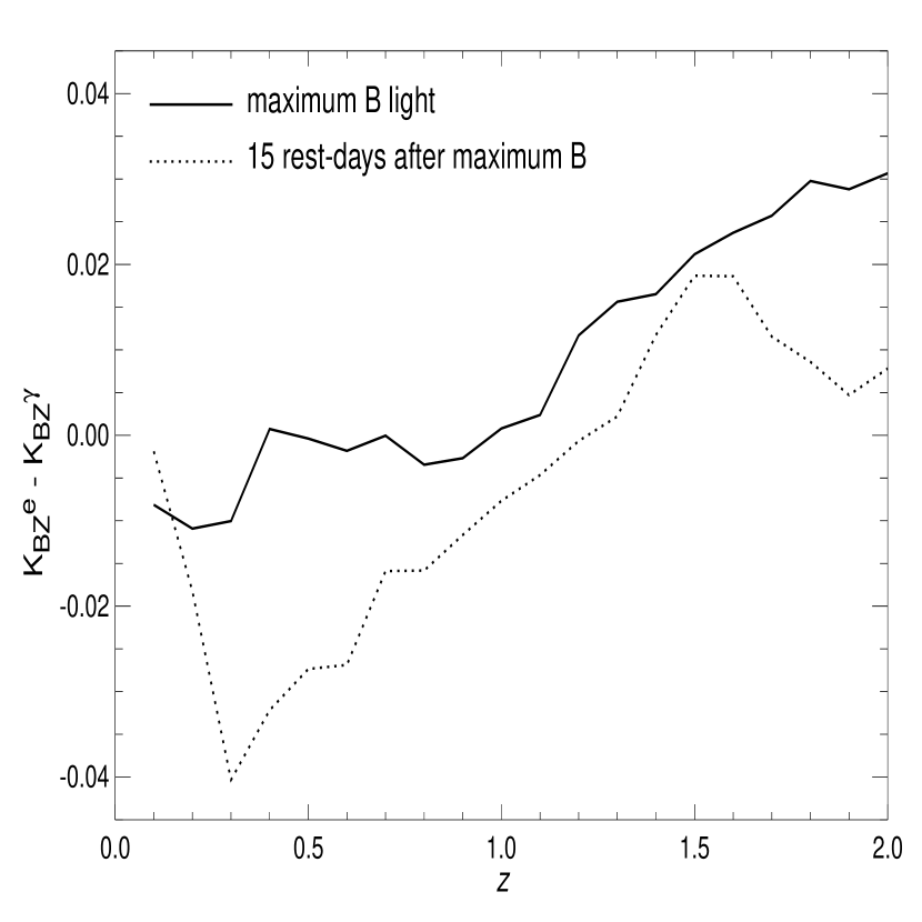
Figure 15: $K_{BZ}^{\epsilon}-K_{BZ}^{\gamma}$ for a standard Type Ia supernova at $B$ maximum and 15 days after maximum as a function of redshift. Measurements in $I$ and bluer filters for $z<1$ supernovae and $J$ and redder filters for $z>1.5$ would provide a better match of observed spectral regions.

To illustrate, in Figure 15 we plot $K_{BZ}^{\epsilon}-K_{BZ}^{\gamma}$ (where $Z$ refers to the passband and not redshift) for a standard Type Ia supernova at $B$ maximum and 15 rest-frame days after maximum out to $z=2$. The differences are close to zero at $z\sim 1.1$ where $B(\lambda/(1+z))\sim Z(\lambda)$. Beyond this optimal redshift, the differences can be $>0.01$ magnitudes. The redder color of the supernova at the later epoch gives relatively larger photon $K$-corrections over almost all redshifts.

The similarity in the two $K$-corrections is due to two competing terms that nearly cancel. A photon $K$-correction is $1+z$ brighter because the supernova does not suffer redshifting energy loss. However, the zeropoint of the redder filter used to observe the redshifted supernova is larger since an A0V photon spectrum is flatter than its energy spectrum. This makes the observed supernova magnitude numerically fainter. Consider the special case where $S_{y}(\lambda)=S_{x}(\lambda/(1+z))$. With perfect filter-matching the specifics of the supernova spectrum are unimportant and the $K$-corrections depend on the zeropoints:

$$K_{xy}^{\epsilon} = -2.5\log\left(\frac{\int{\cal Z}^{\epsilon}_{x}(\lambda)S_{x}(\lambda)d\lambda}{\int{\cal Z}^{\epsilon}_{y}(\lambda)S_{y}(\lambda)d\lambda}\right)$$ (A5)

$$K_{xy}^{\gamma} = -2.5\log\left(\frac{(1+z)\int\lambda{\cal Z}^{\gamma}_{x}(\lambda)S_{x}(\lambda)d\lambda}{\int\lambda{\cal Z}^{\gamma}_{y}(\lambda)S_{y}(\lambda)d\lambda}\right)$$ (A6)

$$= -2.5\log\left(\frac{(1+z)<\lambda_{x}>\int{\cal Z}^{\gamma}_{x}(\lambda)S_{x}(\lambda)d\lambda}{<\lambda_{y}>\int{\cal Z}^{\gamma}_{y}(\lambda)S_{y}(\lambda)d\lambda}\right)$$ (A7)

where $<\lambda>$ is the effective wavelength of the standard through the filter. As long as the standard star is well behaved, we expect the effective wavelength of the redshifted filter to be $1+z$ greater then that of the restframe filter $<\lambda_{y}>\sim(1+z)<\lambda_{x}>$ so that

$$K_{xy}^{\gamma}\sim-2.5\log\left(\frac{\int{\cal Z}^{\epsilon}_{x}(\lambda)S_{x}(\lambda)d\lambda}{\int{\cal Z}^{\epsilon}_{y}(\lambda)S_{y}(\lambda)d\lambda}\right)=K_{xy}^{\epsilon}.$$ (A8)

Choosing filters that accept the same spectral region at both low and high redshifts not only reduces errors but also reduces the difference between energy and photon $K$-corrections.

The effect of using the “energy” distance modulus in defining the $K$-correction in Equations A1, A3, and A4 are seen in the open-filter $K$-corrections. When $S_{x}=S_{y}=1$, the energy $K$-correction is unnecessary and indeed $K_{xy}^{\epsilon}=0$. For the photon $K$-correction we find $K_{xy}^{\gamma}=-2.5\log{(1+z)}$, the difference between “energy” and “photon” distance moduli.

A simple measure for the difference between single-filter $K$-corrections is the ratio in effective wavelength of a redshifted and unredshifted source through that filter. For example, sources with power-law SED’s have identical photon and energy $K$-corrections. For low-redshift objects the difference in effective wavelength should be very small (unless they have pathological spectra) and thus make little difference in distance determinations. For example, a Type Ia supernova at maximum at $z=0.1$ observed through the $B$-band would have a distance modulus error of 0.02 magnitudes if the wrong $K$-correction were applied.

A.3 Final Notes on $K$-corrections

In this appendix we have shown that the measurements $m_{Y}(z)-M_{X}$ do depend on whether the magnitude system is based on energy or photon flux. Although the “photon luminosity distance” is shorter than the standard luminosity distance, we can still use the relation $m_{Y}(z)=M_{X}+\mu(z)+K_{XY}$ with the appropriate definitions of the $K$-corrections; the ones of Kim et al. (1996) are appropriate. With this definition, the standard equations linking the energy distance modulus to cosmology are applicable. The Johnson-Cousins magnitude system is in fact photon-based. Therefore, the $K^{\gamma}_{XY}$ $K$-correction should and has been used in the supernova cosmology analysis of the SCP. Although application of the incorrect $K$-correction would contribute negligibly to the error budget of the current supernova sample, the distinction is important for precision experiments that require 0.02 magnitude accuracies, such as the Supernova Acceleration Probe. With the choice of well-matched filters, differences between energy and photon $K$-correction can be minimal.

Using the “count” distance modulus based on $d_{\gamma}$ in Equation A1 would provide a more physically satisfying definition of the count $K$-correction. Recall that $\mu^{\epsilon}=\mu^{\gamma}+2.5\log{(1+z)}$. Then the extra $2.5\log{(1+z)}$ in the $K$-correction would give

$$K_{xy}^{\gamma}=-2.5\log\left(\frac{\int\lambda{\cal Z}^{\gamma}_{x}(\lambda)S_{x}(\lambda)d\lambda}{\int\lambda{\cal Z}^{\gamma}_{y}(\lambda)S_{y}(\lambda)d\lambda}\right)+2.5\log\left(\frac{\int\lambda f_{\lambda}(\lambda)S_{x}(\lambda)d\lambda}{\int\lambda^{\prime}f_{\lambda}(\lambda^{\prime})S_{y}((1+z)\lambda^{\prime})d\lambda^{\prime}}\right).$$ (A9)

In other words, the $K$-correction would depend simply on the ratio of supernova photons in the rest-frame filter and a blue-shifted observer filter, and the zeropoint. This methodology would preserve the physical meanings that we associate with both distance modulus and $K$-correction. For simplicity, however, we here adopt the energy distance modulus for both $K$-corrections to be consistent with the literature and to ensure unambiguity when referring to $K$-corrected magnitudes and distance moduli.

Table 1: List of SNe Ia used to create the spectral template

SN Name	Epochs with respect to maximum light	References
1981B	0,17,20,26,35,49,58,64	1
1989B	-7,-5,-3,-2,-1,3,5,8,9,11,12,13,14,15,16,17,18,19	2
1990N	-14,-7,7,14,17,38	3,4,5
1992A	-5,-1,3,5,6,7,9,11,16,17,24,28,37,46,76	6
1994D	-10,-9,-8,-7,-4,-3,2,3,4,5,6,8,11,12,13,14,16,18,20,25	7,8
1990af	-2	9
1992ag	0	9
1992al	-5, 4	9
1992aq	2	9
1992bc	-10	9
1992bh	3	9
1992bl	2	9
1992bo	2	9
1992bp	7	9
1992br	7	9
1992bs	3	9
1992P	0	9
1993H	3, 5	9
1993O	-4, 2	9

References. — (1) Branch et al. (1983), (2) Wells et al. (1994), (3) Leibundgut et al. (1991), (4) Phillips et al. (1992), (5) Mazzali et al. (1993), (6) Kirshner et al. (1993) (7) Meikle et al. (1996), (8) Patat et al. (1996), (9) Courtesy of the Calán/Tololo Supernova Survey. Note that, where applicable, the IUE spectra from Cappellaro et al. (1995) were used in forming the template.

Table 2: $UBVRIJHK$ magnitude differences from the peak $B$-band value for the spectral template

Time	U	B	V	R	I	J	H	K
-20.0	$\infty$	$\infty$	$\infty$	$\infty$	$\infty$	$\infty$	$\infty$	$\infty$
-15.0	2.16	2.37	2.71	2.66	3.11	3.27	3.45	3.28
-10.0	0.43	0.83	1.13	0.84	1.11	1.69	1.87	1.70
-5.0	-0.25	0.13	0.26	0.21	0.48	0.82	1.00	0.83
0.0	-0.22	0.00	0.06	0.07	0.42	0.62	0.80	0.63
5.0	0.13	0.16	0.08	0.05	0.53	0.72	0.90	0.73
10.0	0.75	0.55	0.27	0.41	0.87	0.82	1.00	0.83
15.0	1.45	1.05	0.53	0.67	1.00	1.86	1.13	1.14
20.0	2.15	1.59	0.76	0.66	0.77	2.26	0.93	0.90
25.0	2.65	2.08	1.03	0.81	0.72	1.94	0.73	0.73
30.0	2.91	2.49	1.50	1.09	0.87	1.52	0.57	0.68
35.0	3.03	2.78	1.85	1.42	1.30	1.64	0.88	1.00
40.0	3.15	2.99	2.12	1.67	1.63	1.93	1.17	1.33
45.0	3.26	3.15	2.34	1.88	1.88	2.42	1.46	1.60
50.0	3.37	3.25	2.50	2.02	2.03	2.91	1.75	1.88
55.0	3.45	3.33	2.63	2.19	2.23	3.21	1.95	2.08
60.0	3.53	3.41	2.77	2.37	2.44	3.51	2.15	2.28
65.0	3.62	3.50	2.92	2.45	2.53	3.81	2.33	2.46
70.0	3.70	3.58	3.06	2.54	2.61	4.12	2.52	2.64

Table 3: $K_{BB}(z=0.1)$ for two SNe Ia

	SN 1994D			SN 1992A
$t-t_{0}$	$U-B$	$B-V$	$K_{BB}(z=0.1)$	$U-B$	$B-V$	$K_{BB}(z=0.1)$
-5	-0.6	-0.07	-0.04	-0.3	-0.03	0.09
0	-0.5	-0.08	-0.02	-0.3	-0.01	0.07
5	-0.3	0.04	0.06	-0.1	0.26	0.15
10	-0.2	0.22	0.10	0.1	0.40	0.24
15	0.0	0.56	0.20	0.3	0.74	0.34
20	0.2	0.90	0.33	0.4	1.11	0.42

Figure 3: Top panel: Rest-frame $B-V$ color curve for a $s=1.0$ SN Ia. Bottom panel: $K$-corrections for a $s=1.0$ SN Ia at a variety of redshifts. Note the strong similarity between the color curve and the $K$-corrections.

Figure 5: $K_{BR}$ for a $z=0.35$ SN Ia with $s=1.0$ along with three other sets of $K$-corrections. These $K$-corrections were calculated by forcing the spectra within 10 days of a given epoch on the light curve (maximum light, $+10$ days and $+20$ days) to have the same colors as the SN Ia has at that epoch. The difference in the $K$-corrections is, at most, 0.05 mag over the entire 20 day window and $\lesssim$ 0.02 mag for a 10 day window.

Figure 6: A weekly sampling of the spectral template from two weeks before to four weeks after maximum light. The spectra and light curves are available at: http://www.supernova.lbl.gov/$\sim$nugent/spectra.html

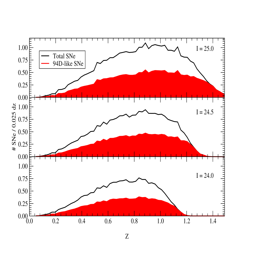
Figure 9: Same as Figure 8 except for an $I$-band search only covering 1 square degree. Here this bias is moved out to $z>0.9$ as that is where the restframe $U$-band light enters the $I$-band filter.

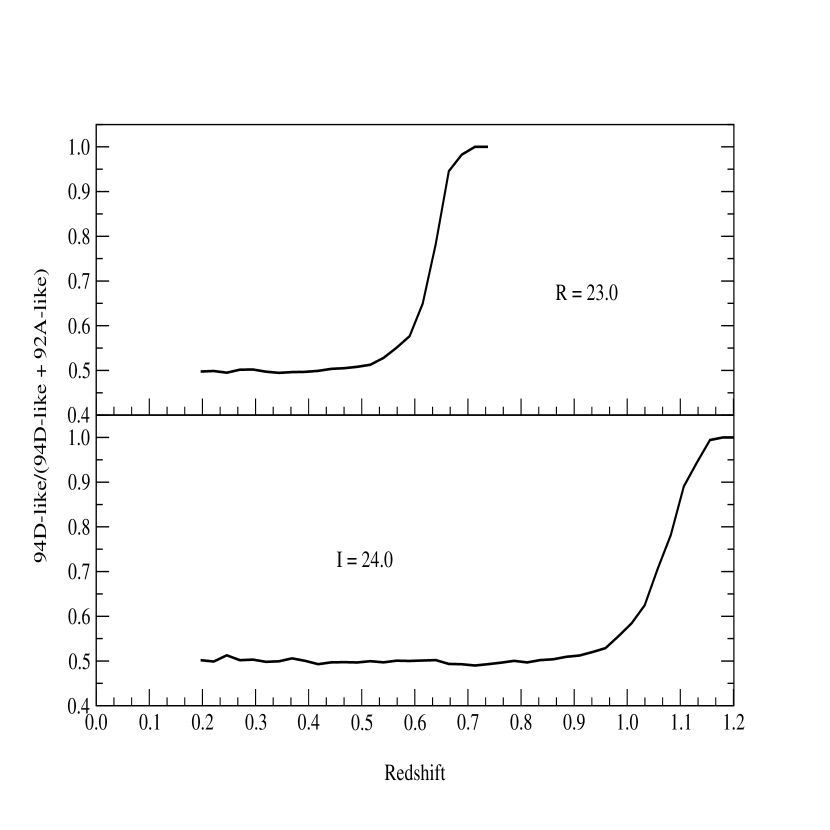
Figure 10: The data from Figures 8 and 9 presented as the ratio of SN 1994D-like supernovae to the total number of supernovae found just the $R$=23.0 and $I$=24.0 limiting magnitude searches.

References

- Ajhar et al. (2001) Ajhar, E. A., Tonry, J. L., Blakeslee, J. P., Riess, A. G., & Schmidt, B. P. 2001, ApJ, 559, 584
- Aldering et al. (1998) Aldering, G. et al. 1998, IAU Circ. No. 7046
- Branch et al. (1981) Branch, D., Falk, S. W., McCall, M. L., Rybski, P., Uomoto, A. K., & Wills, B. J. 1981, ApJ, 244, 780
- Branch, Fisher & Nugent (1993) Branch, D., Fisher, A., & Nugent, P. 1993, AJ, 106, 2383
- Branch et al. (1983) Branch, D., Lacy, C. H., McCall, M. L., Sutherland, P. G., Uomoto, A., Wheeler, J. C., & Wills, B. J. 1983, ApJ, 270, 123
- Branch et al. (1997) Branch, D., Nugent, P., Baron, E., & Fisher, A. 1997, in Thermonuclear Supernova, ed. P. Ruiz-Lapuente, R. Canal, & J.Isern (Dordrecht: Kluwer), 777
- Cappellaro et al. (1995) Cappellaro, E., Turatto, M., & Fernley, J. 1995, IUE - ULDA Access Guide No. 6: Supernovae (The Netherlands: ESA)
- Cardelli et al. (1989) Cardelli, J. A., Clayton, G. C., & Mathis, J. S. 1989, ApJ, 345, 245
- Carroll et al. (1992) Carroll, S. M., Press, W. H., & Turner, E. L. 1992, Ann. Rev. Astro. Astrophys., 30, 499
- Coil et al. (2000) Coil, A. et al. 2000, ApJ, 544, 111
- de Vaucouleurs et al. (1981) de Vaucouleurs, G., de Vaucouleurs, A., Buta, R., Ables, H. D., & Hewitt, A. V. 1981, PASP, 93, 36
- Dreiling & Bell (1980) Dreiling, L. A. & Bell, R. A. 1980, AJ, 241, 736
- Elias et al. (1981) Elias, J. H., Frogel, J. A., Hackwell, J. A., & Persson, S. E. 1981, ApJ, 251, L13
- Filippenko (1997) Filippenko, A. V. 1997, ARA&A, 35, 309
- Filippenko et al. (1992) Filippenko, A. V. et al. 1992, AJ, 104, 1543
- Gilliland, Nugent & Phillips (1999) Gilliland, R. L., Nugent, P. E., & Phillips, M. M. 1999, ApJ, 521, 30
- Goldhaber et al. (2001) Goldhaber, G. et al. 2001, ApJ, 558, 359
- Hamuy et al. (1996) Hamuy, M., Phillips, M. M., Maza, J., Suntzeff, N. B., Schommer, R. A., & Aviles, R. 1996, AJ, 112, 2391
- Hamuy et al. (1993) Hamuy, M., Phillips, M. M., Wells, L., & Maza, J. 1993, PASP, 105, 787
- Hamuy et al. (2000) Hamuy, M., Tragerand, S. C., Pinto, P. A., Phillips, M. M., Schommer, R. A., Ivanov, V., & Suntzeff, N. B. 2000, AJ, 120, 1479
- Höflich et al. (1998) Höflich, P., Wheeler, J. C., & Thielemann, F. K. 1998, ApJ, 495, 617
- Jha et al. (1999) Jha, S. et al. 1999, ApJS, 125, 73
- Johnson & Morgan (1951) Johnson, H. L. & Morgan, W. W. 1951, ApJ, 114, 522
- Johnson & Morgan (1953) —. 1953, ApJ, 117, 313
- Kim et al. (1996) Kim, A., Goobar, A., & Perlmutter, S. 1996, PASP, 108, 190
- Kirshner et al. (1993) Kirshner, R. et al. 1993, ApJ, 415, 589
- Knop (2002) Knop, R. 2002, B.A.A.S., 199, 16.07
- Krisciunas et al. (2001) Krisciunas, K., Phillips, M. M., Stubbs, C., Rest, A., Miknaitis, G., Riess, A. G., Suntzeff, N. B., Roth, M., Persson, S. E., & Freedman, W. L. 2001, AJ, 122, 1616
- Landolt (1973) Landolt, A. U. 1973, AJ, 78, 959
- Landolt (1983) —. 1983, AJ, 88, 439
- Landolt (1992) —. 1992, AJ, 104, 340
- Leibundgut (1988) Leibundgut, B. 1988, PhD thesis, University of Basel
- Leibundgut et al. (1991) Leibundgut, B., Kirshner, R. P., Filippenko, A. V., Shields, J. C., Foltz, C. B., Phillips, M. M., & Sonneborn, G. 1991, ApJ, 371, L23
- Lentz et al. (2000) Lentz, E. J., Baron, E., Branch, D., Hauschildt, P. H., & Nugent, P. E. 2000, ApJ, 530, 966
- Mazzali et al. (1993) Mazzali, P. A., Lucy, L. B., Danziger, I. J., Gouiffes, C., Cappellaro, E., & Turatto, M. 1993, A&A, 269, 423
- Meikle et al. (1996) Meikle, W. P. S. et al. 1996, MNRAS, 281, 263
- Nugent (1997) Nugent, P. 1997, PhD thesis, University of Oklahoma
- Nugent et al. (1997) Nugent, P., Baron, E., Branch, D., Fisher, A., & Hauschildt, P. 1997, ApJ, 485, 812
- Nugent et al. (1995) Nugent, P., Phillips, M., Baron, E., Branch, D., & Hauschildt, P. 1995, ApJ, 455, L147
- Oke & Sandage (1968) Oke, J. B. & Sandage, A. 1968, ApJ, 154, 21
- Patat et al. (1996) Patat, F. et al. 1996, MNRAS, 278, 111
- Perlmutter et al. (1997) Perlmutter, S. et al. 1997, ApJ, 483
- Perlmutter et al. (1998) —. 1998, Nature, 391
- Perlmutter et al. (1999) —. 1999, ApJ, 517, 565
- Phillips (1993) Phillips, M. M. 1993, ApJ, 413, L105
- Phillips et al. (1999) Phillips, M. M., Lira, P., Suntzeff, N. B., Schommer, R. A., Hamuy, M., & Maza, J. 1999, AJ, 118, 1766
- Phillips et al. (1987) Phillips, M. M. et al. 1987, PASP, 99, 592
- Phillips et al. (1992) —. 1992, AJ, 103, 1632
- Richmond et al. (1995) Richmond, M. W. et al. 1995, AJ, 109, 2121
- Riess et al. (1998a) Riess, A. et al. 1998a, AJ, 116, 1009
- Riess et al. (1998b) —. 1998b, AJ, 116, 1009
- Riess et al. (1999a) —. 1999a, AJ, 118, 2675
- Riess et al. (1999b) —. 1999b, AJ, 117, 707
- Riess et al. (1996) Riess, A. G., Press, W. H., & Kirshner, R. P. 1996, ApJ, 473, 588
- Schneider et al. (1983) Schneider, D. P., Gunn, J. E., & Hoessel, J. G. 1983, ApJ, 264, 337
- Strolger et al. (2002) Strolger, L. et al. 2002, ApJ, submitted
- Suntzeff et al. (1999) Suntzeff, N. B. et al. 1999, AJ, 117, 1175
- Tonry (2000) Tonry, J. 2000, private communication
- Tripp & Branch (1999) Tripp, R. & Branch, D. 1999, ApJ, 209, 525
- van den Bergh (1995) van den Bergh, S. 1995, ApJ, 453, L55
- Wells et al. (1994) Wells, L. A. et al. 1994, AJ, 108, 2233