HST STIS observations of four QSO pairs

We present HST  STIS observations of four quasar pairs with redshifts 0.84 $<$ $z_{\rm em}$ $<$ 1.56 and angular separation 2–3 arcmin corresponding to $\sim\,$1$-$1.5$h^{-1}_{50}$ Mpc transverse proper distance at $z$ $\sim$ 0.9. We study the distribution of velocity differences between nearest neighbor Hi  Lyman-$\alpha$ absorption lines detected in the spectra of adjacent QSOs in order to search for the possible correlation caused by the extent or the clustering properties of the structures traced by the absorption lines over such a scale. The significance of the correlation signal is determined by comparison with Monte-Carlo simulations of spectra with randomly distributed absorption lines. We find an excess of lines with a velocity separation smaller than $\Delta V$ = 500 km s^-1 significant at the 99.97% level. This clearly shows that the Lyman-$\alpha$ forest is correlated on scales larger than 1$\,h^{-1}_{50}$ Mpc at $z$ $\sim$ 1. However, out of the 20 detected coincidences within this velocity bin, 12 have $\Delta V$ $>$ 200 km s^-1. This probably reflects the fact that the scale probed by our observations is not related to the real size of individual absorbers but rather to large scale correlation. Statistics are too small to conclude about any difference between pairs separated by either 2 or 3 arcmin. A damped Lyman-$\alpha$ system is detected at $z_{\rm abs}$ = 1.2412 toward LBQS 0019$-$0145A with log $N$(Hi) $\sim$ 20.5. From the absence of Znii absorption, we derive a metallicity relative to solar [Zn/H] $<$ $-$1.75.

1 Introduction

Recent $N$-body numerical simulations reproduce successfully the global characteristics of the neutral hydrogen absorptions observed in quasar spectra, the so-called Lyman-$\alpha$ forest (Cen et al. 1994; Petitjean et al. 1995, Hernquist et al. 1996; Zhang et al. 1995; Mücket et al. 1996; Miralda-Escudé et al. 1996; Bond & Wadsley 1998). The absorptions arise from density inhomogeneities in a smooth all-pervading intergalactic medium. Simulations show that the intergalatic gas traces the potential wells of the dark matter well at high redshift. It is therefore possible to constrain the characteristics of the dark-matter density field from observation of the Lyman-$\alpha$ forest along a single line of sight (Croft et al. 2000). The addition of transverse information from observation of QSO pairs or more generally groups of quasars at small projected separation in the sky will probably revolutionize this field in the next few years (Petitjean 1997). Indeed, inversion methods that have been recently implemented show that it is possible to recover the 3D topology of the dark-matter field using a dense network of lines of sight (Nusser & Haehnelt 1998, Pichon et al. 2001, Rollinde et al. 2001).

After the early discovery of common absorptions in pairs of quasars (Shaver et al. 1982, Shaver & Robertson 1983, Weyman & Foltz 1983, Foltz et al. 1984), it was shown that the gaseous complexes giving rise to the absorptions should have large dimensions. In particular, studies of gravitationally lensed quasars (Smette et al. 1992, Smette et al. 1995) yielded a lower limit of 100 $h_{50}^{-1}$ kpc  on the diameter of Lyman-$\alpha$ absorbers. Similar results were obtained from pairs of quasars with small separation (Bechtold et al. 1994; Dinshaw et al. 1994; Petitjean et al. 1998, D’Odorico et al. 1998; Monier et al. 1998). Larger separations have been investigated by Crotts & Fang (1998), Dinshaw et al. (1998), Monier et al. (1999) and Williger et al. (2000). All studies conclude that absorptions are correlated on scales larger than 500 $h_{50}^{-1}$ kpc.

Unlike the case of QSO pairs with small angular separations where the correlation can be explained by the fact that the lines of sight intercept the same absorber, the correlation for larger separations is certainly due to the clustering properties of distinct clouds. When observing triplets of quasars separated by 1 to 2 arcmin on the sky, corresponding to $\sim\,$0.5 to 1 Mpc proper distance scales, both Crotts & Fang (1998) and Young et al. (2001) find statistically significant triple coincidences that they interpret as the presence of sheetlike structures along which inhomogeneous absorbers cluster.

The number of such experiments is small however and it is important to increase the statistics. Here we present HST observations of four pairs of quasars. The $\sim\,$2 and $\sim\,$3 arcmin angular separations between the two quasars of each pair probes scales between 1.0 and 1.5 $h^{-1}_{50}$ Mpc proper distance at $z$ $\sim$ 1. This is where the transition between individual halos and filamentary or sheet-like large scale structures is expected (Mücket et al. 1996, Charlton 1997).

We describe the observations in Sect. 2 and comment on individual metal line systems in Sect. 3. Correlations between metal line and Lyman-$\alpha$ systems are respectively discussed in Sect. 4 and 5. Conclusions are drawn in Sect. 6.

2 Observations

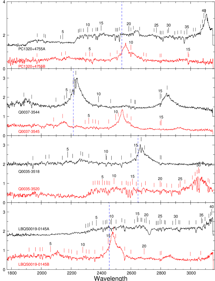
Figure 1: HST  STIS spectra of the eight observed quasars. The tick marks indicate significant ($>$4$\sigma$) absorption features. The vertical dashed lines mark the red limit of the wavelength range for the selection of the Lyman-$\alpha$  lines. This limit is defined by the wavelength at which a line lies at more than 3000 km s^-1 blueward of the Lyman-$\alpha$ emission line of the lowest redshift quasar in a given pair.

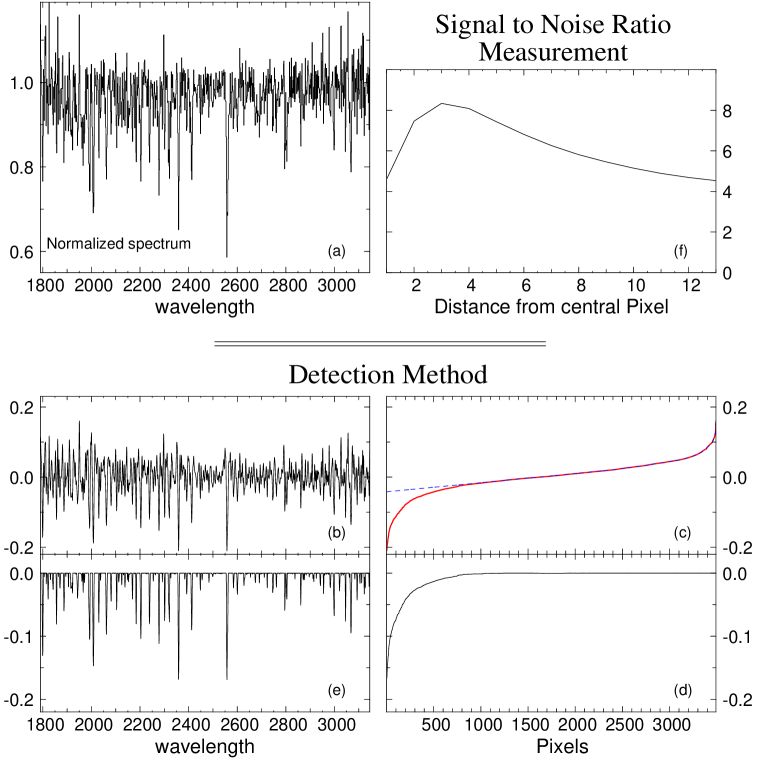
Figure 2: Illustration of the procedure used to detect absorption lines. Panel (a) represents the original normalized spectrum which is wavelet filtered to select scales characteristic of the absorption lines. The filtered spectrum is shown in panel b. All pixels in the spectrum are sorted according to their value (panel c). Low values correspond to absorption and high values to spikes; the intermediate values are dominated by noise which is fitted by the dashed line in panel (c). This level of noise is subtracted to each pixel to give the new distribution of panel (d) and pixels are reordered. The resulting spectrum is shown in panel (e). This spectrum is used only to select the regions where absorption lines are detected. The equivalent width of each absorption feature is measured in the original spectrum. For each line, the signal to noise ratio is plotted as a function of the distance to the central pixel (panel f). The S/N ratio of the line is taken at the maximum of the curve.

Table 1: List of observed QSOs

Object name	zem	$\Delta\theta$	$\Delta z$	$<\rm{S}>$
LBQS0019-0145A	1.59
LBQS0019-0145B	1.04	3.3	$0.70\,-\,1.01$	1640
Q0035-3518	1.20
Q0035-3520	1.52	3.4	$0.69\,-\,1.17$	1710
Q0037-3545	1.10
Q0037-3544	0.84	1.7	$0.59\,-\,0.82$	810
PC1320+4755A	1.56
PC1320+4755B	1.11	1.9	$0.62\,-\,1.08$	940

Observations were carried out on the Hubble Space Telescope  using the Space Telescope Imaging Spectrograph (STIS) with the G230L grating and the Near-UV-MAMA detector. This configuration yields a mean spectral resolution of R = 700 (FWHM = 3.4 Å at $\lambda$ = 2374 Å) and a wavelength coverage from 1570 Å to 3180 Å. The observations were reduced at the Goddard Space Flight Center with the STIS Investigation Definition Team (IDT) version of CALSTIS (Lindler 1998). Standard reduction and calibration were used. Special care was taken to determine accurately the background due to the sky and the dark current. The zero point of the wavelength scale for individual exposures was determined requiring the Galatic interstellar absorptions to occur at rest. The correction can always be performed because the Galactic Mgii doublet is well detected in every single spectrum. When the Feii lines were also detected we checked that the dispersion in the zero point is smaller than the spectral resolution. The resulting spectra are shown in Fig. 1. The quasar  continuum was fitted with Gaussian profiles for emission lines and simple cubic splines in regions between emission lines. The best fit was found by varying the position of the control points of the cubic splines. The resulting continuum was slightly manually adjusted in regions that were poorly fitted as for example near broad emission lines and Lyman limits. The detection of absorption lines in the normalized spectrum was performed by filtering each spectrum to improve the contrast between lines and noise. This has been performed by successively applying a wavelet filter and an “upgraded” median filter to the spectrum.

We used for the wavelet filter B3-spline scaling functions. This filter selects the wavelength scales corresponding to the width of the absorption lines  (see panel b of Fig. 2). Pixels from the wavelet filtered spectra are sorted in increasing order keeping trace of the pixel permutations. The distribution of the pixel values is shown in panel (c) of Fig. 2. A lower limit of the level of noise in each pixel can be estimated (dashed line) and substracted to the real pixel value (panel d in Fig. 2). Pixels are then reordered and the resulting spectrum is shown in panel (e) of Fig. 2. This filtered spectrum is used to define regions where possible absorption lines are present using a threshold defined so that no line is lost in the next step. We then compute in the original spectrum the equivalent width and the associated noise over each of these regions and select only those with an equivalent width to noise ratio larger than 2. The corresponding regions are then fitted with a Voigt profile fitting program to derive the position of absorption features. This software makes a $\chi^{2}$ minimisation in each region adding lines until the reduced $\chi^{2}$ reaches a value lower than or equal to 1.

For each absorption feature, we calculate the equivalent width in windows centered on the minimum of the line and of widths an increasing number of pixels. The signal-to-noise ratio computed from the noise spectrum is plotted as a function of the distance to the central pixel (panel f of Fig. 2). The S/N ratio of the line was taken at the maximum of the curve and the equivalent width was computed by integrating the fitted profile. The lines with S/N ratio greater than 4 are listed with their identification in Tables 2 to 5. In these tables, uncertain positions or identifications are indicated by a colon.

3 Comments on individual metal line systems

Table 2: Line list for the pair LBQS0019-0145AB

Table 3: Line list for the pair LBQS0035-3518 & Q0035-3520

Table 4: Line list for the pair Q0037-3544 & Q0037-3545

Table 5: Line list for the pair PC1320+4755AB

In this Section we comment on the intervening metal line systems identified in the spectra. To refer to an absorption feature, we use the numbering given in Tables 2 to 5.

3.1 LBQS 0019$-$0145A   z_em = 1.59

The HST data on this quasar have been complemented with a high resolution (R $\sim$ 40000) UVES spectrum covering the wavelength ranges 3900$-$5200 Å and 5450$-$9300 Å. The exposure time was two hours.

3.1.1 $z_{\rm abs}$ = 0.6514

The strong absorption feature #13 at $\lambda$2559.23 cannot be explained by Lyman-$\beta$ at $z_{\rm abs}$ = 1.4976 alone because the corresponding equivalent width is too large. As there is a strong Civ system at $z_{\rm abs}$ = 0.65142 in the spectrum of LBQS 0019$-$0145B, we tentatively note that the additional absorption could be due to Civ at $z_{\rm abs}$ = 0.6514. The corresponding Lyman-$\alpha$ absorption is unfortunately redshifted below the Lyman limit of the $z_{\rm abs}$ = 1.4976 system. Mgii$\lambda$2803 at this redshift is not detected in the UVES spectrum down to $w_{\rm obs}=35$ mÅ.

3.1.2 $z_{\mathrm{abs}}$ = 0.6953

Figure 3: Metal absorption lines at $z$ = 0.6953 (left column) and $z$ = 1.2412 (right column, damped Lyman-$\alpha$ system) in the LBQS 0019$-$0145A UVES spectrum.

Mgii$\lambda$2796 ($w_{\mathrm{r}}$$\sim$0.8 Å), Feii$\lambda$2382 ($w_{\mathrm{r}}$$\sim$0.5 Å), Mgi$\lambda$2852 and Caii absorptions are detected at this redshift in the UVES spectrum in addition to Alii$\lambda$1670 (line #28) which is detected in the HST  spectrum. Unfortunately, the Hi$\lambda$1215 line is redshifted at $\lambda$ = 2060 Å, below the Lyman limit of the $z_{\rm abs}$ = 1.4976 system.

The profile of the Mgii  and Feii absorptions consists of two main absorption features approximately $100\,\mathrm{km\leavevmode\nobreak\ s^{-1}}$ apart and separated by a sharp drop in optical depth near the center (see Fig. 3). As described by Bond et al. (2001), and despite the moderate Mgii$\lambda$2796  equivalent width, this profile may indicate that the line of sight intercepts a superwind.

3.1.3 $z_{\mathrm{abs}}$ = 1.2412

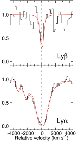
Figure 4: Lyman-$\alpha$ and Lyman-$\beta$  absorptions centered at $z_{\mathrm{abs}}$ = 1.2412 toward LBQS 0019$-$0145A. The continuous curve is the best fit to the two Hi absorptions obtained with log $N$(Hi) $\sim$ 20.5.

Strong Hi$\lambda$1215 (line #21), Hi$\lambda$1025, Siii, Siiii$\lambda$1206, Siiv, Nv and Cii$\lambda$1334  absorptions associated with this system are detected in the HST  spectrum. Additional Mgii, Mgi$\lambda$2852, Feii  and Aliii$\lambda$1854, 1862 absorptions are seen in the UVES spectrum (see Fig. 3). Despite the low resolution of the HST spectrum, damped wings are clearly seen in the case of the Lyman-$\alpha$ line. The simultaneous fit of the Lyman-$\alpha$, and Lyman-$\beta$ absorptions gives log $N$(Hi)$\sim$20.5 (see Fig. 4). The observed Feii and Mgii lines are heavily saturated so that only a lower limit on the column densities can be derived, log $N$(Feii  & Mgii)$>$15. Znii  is not detected with log $N$(Znii) $<\nolinebreak 11.4$ implying that metallicity relative to solar, [Zn/H] $<$ $-$1.75, is one of the smallest observed at low redshift (see e.g. Ledoux et al. 2001). Note that the large column density found for Mgii implies that the neutral part of the system cannot account for all the Mgii we see.

As for the system at $z_{\mathrm{abs}}$ = 0.6953, the profiles of the absorptions consist of two main components separated by about 50 km s^-1. This again may indicate that the line of sight intercepts a superwind.

3.1.4 $z_{\mathrm{abs}}$ = 1.3088

The system is unambiguously identified by sharp Mgii$\lambda$2796, 2803 absorptions ($w_{\mathrm{r}}$$\sim$0.07 Å) detected in the UVES spectrum. The Lyman-$\alpha$ absorption is blended with Mgii$\lambda$2796 from the interstellar medium.

3.1.5 $z_{\mathrm{abs}}$ = 1.4976

This strong system is detected by Hi$\lambda$1215, 1025, 972, 949, 937 and Ciii$\lambda$977 absorptions. It is at the origin of the Lyman limit at $\lambda$ $\sim$ 2270 Å  and therefore log $N$(Hi) $>$ 18. A possible Mgii$\lambda$2796 absorption line is present in the UVES spectrum with $w_{\rm obs}$ $\sim$ 25 mÅ.

3.2 LBQS 0019$-$0145B   z_em = 1.04

Only one metal line system along this line of sight is detected at $z_{\rm abs}$ = 0.6513 by Hi$\lambda$1215, Civ$\lambda$1548, 1550 and Siiv$\lambda$1393, 1402 absorptions.

3.3 Q 0035$-$3518   z_em = 1.20

3.3.1 $z_{\mathrm{abs}}$ = 1.088

Strong Hi$\lambda$972, 1025, 1215  and Siii$\lambda$1260 absorptions are detected in this system. The latter line is probably blended with an other Lyman-$\alpha$ line however. Moreover, an absorption feature detected at the 2.5$\sigma$ level is observed at the expected position of Cii$\lambda$1334  at $\lambda\mbox{$\sim$}2785$ Å.

3.3.2 $z_{\mathrm{abs}}$ = 1.1954

This system is at slightly larger redshift than the quasar ($\sim\,$+1200 km s^-1). It shows strong associated Ovi absorption. Nv$\lambda$1238 is detected at the 2.5$\sigma$ level.

3.4 Q 0035$-$3520   z_em = 1.52

The four metal line systems detected in this quasar are all within 3500 km s^-1 from the emission redshift of the quasar. As they are approximately at the same redshift, their Lyman-$\beta$  and Ovi absorptions are blended. The resulting blend corresponds to the four strong features seen at $\lambda\mbox{$\sim$}$2600 Å  in Fig. 1.

3.4.1 $z_{\mathrm{abs}}$ = 1.4927

The Lyman-$\beta$ line of this system is observed at $\lambda\mbox{$\sim$}$2550 Å, but is below the 4$\sigma$ detection limit. As no other metal line is detected, the Ciii$\lambda$977 identification is tentative and the feature at $\lambda$2437.38 could be a blend of Lyman-$\gamma$ at $z_{\rm abs}$ = 1.50621 and Lyman-$\alpha$ at $z_{\rm abs}$ = 1.00492.

3.4.2 $z_{\mathrm{abs}}$ = 1.50362

This system consists of Hi$\lambda$949, 972, 1025, 1215, Ovi  and Ciii$\lambda$977  absorptions. A feature is also observed at the expected wavelength  of the associated Siiii$\lambda$1206 absorption ($\lambda\mbox{$\sim$}$3020 Å).

3.4.3 $z_{\mathrm{abs}}$ = 1.5118

Hi$\lambda$1025, 1215, Ovi, Ciii$\lambda$977 and Siiii$\lambda$1206 are observed at this redshift.

3.4.4 $z_{\mathrm{abs}}$ = 1.5158

This system has all the characteristics of an associated system with very strong Nv  and Ovi  lines. Therefore the Niii  and Ciii identifications are tentative.

3.5 Q 0037$-$3544   z_em = 0.84

3.5.1 $z_{\mathrm{abs}}$ = 0.5922

Strong Hi$\lambda$1215  and Civ  absorptions are detected. Siiv$\lambda$1393, 1402  are redshifted at $\lambda$2219.4 and 2231.31 Å  (lines #8 and #9). Given the strengths of the corresponding absorption features, it is most probable that the two Siiv lines are blended with additional Lyman-$\alpha$ lines. An absorption feature is detected at the expected position of Siiii$\lambda$1206  ($\lambda\mbox{$\sim$}$1920 Å) but is below the 4$\sigma$ threshold.

3.5.2 $z_{\mathrm{abs}}$ = 0.6961

This system consists of a Civ doublet detected outside the Lyman-$\alpha$ forest. The Lyman-$\alpha$ absorption is observed at wavelength 2062 Å, but is below the 4$\sigma$ threshold.

3.5.3 $z_{\mathrm{abs}}$ = 0.8364

Hi$\lambda$1215, Siiii$\lambda$1206  and Civ absorptions are observed at this redshift. Moreover, a feature is observed at the expected position of Siii$\lambda$1260 ($\lambda\mbox{$\sim$}$2316 Å).

3.6 Q 0037$-$3545   z_em = 1.10

We do not identify any metal line system along this line of sight.

3.7 PC 1320+4755A   z_em = 1.56

3.7.1 $z_{\mathrm{abs}}$ = 1.0762

Strong Hi$\lambda$949, 972, 1025, 1215, Ciii$\lambda$977, Siiv, Siii$\lambda$1260  and Cii$\lambda$1334  absorptions are detected at this redshift. Additional features are observed at the expected wavelengths of the associated Niii989 ($\lambda\mbox{$\sim$}$2055 Å) and Siii$\lambda$1190, 1993 ($\lambda\mbox{$\sim$}$2470 & 2480 Å). This system is at the origin of the Lyman limit seen at $\sim\,$1890 Å  and therefore log $N$(Hi) $>$ 18.

3.7.2 $z_{\mathrm{abs}}$ = 1.4329

Strong Hi (from Lyman-$\alpha$  to Lyman-$\zeta$) , Ovi, Siiii$\lambda$1206  and Siii$\lambda$1260 absorptions are observed. From the partial Lyman limit seen at $\sim\,$2210 Å, we derive log $N$(Hi) $\sim$ 17.3.

3.8 PC 1320+4755B   z_em = 1.11

Only one metal line system is detected along this line of sight at $z_{\rm abs}$ = 0.9270. It consists of Hi$\lambda$1215, Siiii$\lambda$1206, Siiv  and Civ  absorptions. A feature is observed at the position of the associated Siii$\lambda$1260 ($\lambda\mbox{$\sim$}$2430 Å).

4 Correlation of metal line systems

Table 6: List of metal lines for the four pairs

Ident.	$z_{\rm{abs}}$		$w_{\rm{obs}}$		Ident.	$z_{\rm{abs}}$		$w_{\rm{obs}}$
		mina	maxa	4$\sigma^{\rm b}$			mina	maxa	4$\sigma^{\rm b}$
LBQS0019-0145A  (zem=1.59)					LBQS0019-0145B  (zem=1.04)
				24.73	Lyman-$\alpha$	0.65158		2.01	0.70
Civ$\lambda$1548:	0.65171	1.54	1.67	0.54	Civ$\lambda$1548	0.65158		2.08	0.40
Alii$\lambda$1670	0.69423		0.97	0.69					0.53
Q0035-3518  (zem=1.20)					Q0035-3520  (zem=1.52)
Lyman-$\alpha$	1.08706		3.74	0.54					0.58
Siii$\lambda$1260	1.08706	0.00	1.56	0.42					0.61
Lyman-$\alpha$	1.19540		1.85	0.30					0.65
Ovi$\lambda$1031	1.19540		1.12	0.53					1.33
Q0037-3544  (zem=0.84)					Q0037-3545  (zem=1.10)
Lyman-$\alpha$	0.59223		2.47	0.79					0.96
Civ$\lambda$1548	0.59223		0.61	0.56					0.55
Civ$\lambda$1548	0.83642		0.36	0.37					0.72
PC1320+4755A  (zem=1.56)					PC1320+4755B  (zem=1.11)
				0.52	Lyman-$\alpha$	0.92572		4.28	0.78
				0.79	Civ$\lambda$1548	0.92572		2.75	1.05
Lyman-$\alpha$	1.07581	2.91	3.28	0.41					0.65
Siii$\lambda$1260	1.07581		1.07	0.44					0.58
Siiv$\lambda$1393	1.07581		0.78	0.68					1.05
rma minimum an maximum equivalent widths taking into account blending
rmb four sigma detection limit

We summarize in Table 6 the metal line systems seen along one line of sight for which the corresponding absorption along the adjacent line of sight could be observed. In case of blending, $w_{\rm obs,min}$ and $w_{\rm obs,max}$ are the minimum and maximum equivalent width of the transition. These values are computed using consistency arguments relating the equivalent widths of lines observed in the same system (see examples in Sect. 5.1). The 4$\sigma$ detection limits are also indicated.

There are only 6 metal line systems which have all $w_{\rm r}$(Lyman-$\alpha$) $>$ 1 Å. Apart from the Civ system at $z_{\rm abs}$ = 0.65 toward LBQS 0019$-$0145B which may have a coincident absorption in LBQS 0019$-$0145A (see Sect. 3.1.1), none of the other systems are detected along the adjacent line of sight down to a 4$\sigma$ limit of $w_{\rm r}$(Lyman-$\alpha$) $<$ 0.40 Å. As the system at $z_{\rm abs}$ = 1.19 toward Q 0035$-$3518 could be associated with the quasar, this means that out of 5 intervening metal line systems with $w_{\rm r}$(Lyman-$\alpha$) $>$ 1 Å, only one is present in the two lines of sight.

Correlation of Civ systems however has been claimed on large scales at high redshift (e.g. Williger et al. 1996). Moreover, of the five $w_{\rm r}$ $>$ 0.4 Å  Lyman-$\alpha$ systems seen at the same $z$ $\sim$ 2 redshift in the three spectra of KP 76, 77 and 78 (triple hits over 2-3 arcmin separations), two show associated Civ although Civ  is seen only in about one $w_{\rm r}$ $>$ 0.4 Å  Lyman-$\alpha$ system out of ten (Crotts & Fang 1998). All this may indicate that the transverse clustering of Civ  systems is less pronounced at $z$ $\sim$ 1 than at $z$ $\sim$ 2 (see also D’Odorico et al. 2002).

5 Correlation in the Lyman-$\alpha$ forest

Table 7: List of Lyman-$\alpha$ lines for the four pairs

	$z_{\rm{abs}}$	$w_{r}^{\rm{min}}$	$w_{r}^{\rm{max}}$	$w_{r,4\sigma}^{\rm a}$		$z_{\rm{abs}}$	$w_{r}^{\rm{min}}$	$w_{r}^{\rm{max}}$	$w_{r,4\sigma}^{\rm a}$
		(Å)	(Å)	(Å)			(Å)	(Å)	(Å)
Q0019-0145A					Q0019-0145B
				5.64	5	0.69604		0.84	0.53
				1.70	7	0.79664		0.36	0.31
				1.50	8	0.81211		0.71	0.41
				0.94	9	0.84196		0.46	0.35
				0.91	10	0.87377		0.56	0.31
				0.71	12	0.90834	0.55	0.63	0.39
3	0.91117	0.28	0.49	0.63					0.38
				0.51	13	0.94027		0.86	0.30
5	0.94886		1.23	0.59					0.42
				0.49	14	0.98403		0.84	0.34
6	0.98569		1.64	0.40					0.30
8	1.00660		0.56	0.39					0.26
				0.30	15	1.01375		0.17	0.17
Q0035-3518					Q0035-3520
1	0.59890		2.30	0.85					1.31
2	0.66948	0.83	1.21	0.76					1.29
5	0.79062		0.85	0.54					1.11
6	0.81789		0.61	0.53					1.01
9	0.90694		0.60	0.38					0.56
				0.57	1	0.93067		2.26	0.57
10	1.00178		0.69	0.30					0.33
				0.42	7	1.00497	0.42	0.82	0.41
11	1.00510		0.53	0.34					0.33
12	1.03169		0.88	0.36					0.39
				0.44	10	1.04595	0.00	1.01	0.41
13	1.08706		1.79	0.36					0.41
				0.38	11	1.08927	0.64	1.13	0.40
15	1.16567	0.00	0.72	0.26					0.38
				0.21	16	1.16861		0.53	0.30
Q0037-3544					Q0037-3545
2	0.59223		1.55	0.67					0.84
				0.56	1	0.71350		0.89	0.47
3	0.72613		1.06	0.75					0.69
				0.50	2	0.76277		0.43	0.38
4	0.77194		0.47	0.37					0.32
5	0.78490		0.36	0.34					0.35
6	0.80395		0.59	0.33					0.49
				0.31	3	0.82163		0.76	0.51
PC1320+4755A					PC1320+4755B
				1.35	1	0.62172		2.21	1.43
1	0.62281	0.94	1.72	1.14					1.22
2	0.66003	0.27	0.89	1.07					1.08
3	0.66821	1.67	1.67	1.31					1.18
				1.65	2	0.75664		1.06	1.09
5	0.76329	0.29	0.51	0.99					0.65
				1.14	3	0.77902		0.70	0.70
6	0.84951		0.96	0.47					0.72
7	0.85514		0.93	0.34					0.58
				0.32	4	0.89023		0.62	0.46
				0.48	6	0.92572		2.22	0.72
11	0.92713	0.97	1.04	0.40					0.61
14	0.95579		1.78	0.43					0.80
15	0.97471		0.37	0.29					0.54
				0.36	7	1.02501		0.64	0.51
19	1.07581	1.40	1.58	0.22					0.41
				0.33	9	1.08477		0.71	0.38
a calculated using the width of the line detected along
either line of sight.

5.1 The Lyman-$\alpha$ line list

From the line lists obtained as described in Sect. 2 and given in Tables 2 to 5, we have extracted for each pair of QSOs, a master line-list of Lyman-$\alpha$ lines based on several criteria: (i) we include all isolated lines when no other identification is found; (ii) the lines must be at more than 3000 km s^-1 blueward of the two Lyman-$\alpha$ emission lines; (iii) we use physical consistency arguments to infer the presence of Lyman-$\alpha$ lines blended with metal lines (for example Civ$\lambda$1548 cannot be weaker than Civ$\lambda$1550); only limits on the equivalent width can be inferred this way; (iv) we impose some equivalent width threshold. The Lyman-$\alpha$ line list is summarized in Table 7. The columns correspond to: #1 and #6 line number in the spectrum (see Fig. 1); #2 and #7 Lyman-$\alpha$ redshift; #3:#4 and #8:#9 the range in equivalent widths in case of blending (see below); #5 and #10 the 4$\sigma$ equivalent width detection limit using the width of the line detected along either line of sight.

In LBQS 0019$-$0145A, absorption #3 cannot only be Ovi$\lambda$1037 as it has $w_{\rm obs}$ = 2.10 Å  whereas $w_{\rm obs}$(OVI1031) = 1.64 Å. The hidden Lyman-$\alpha$ line has 0.28 $<$ $w_{\rm obs}$ $<$ 0.49 Å  corresponding to the Ovi doublet ratio ranging from 1 to 2.

Absorption #8 coincides in redshift with Ciii  at $z_{\mathrm{abs}}$ = 1.49672. However, we consider this identification unlikely. Indeed, the line is quite strong ($w_{\rm obs}$ = 1.12 Å) even though the UVES and STIS spectra do not show any other metal lines at this redshift except for a very weak Mgii$\lambda$2796  line system and a 2.5$\sigma$ feature shifted by 1.5 Å from the expected position of Siiii$\lambda$1206. Therefore, we identify this line as Lyman-$\alpha$ at $z_{\mathrm{abs}}$ = 1.00660.

In LBQS 0019$-$0145B, the limits on the equivalent width of the Lyman-$\alpha$ line blended with Siiv$\lambda$1402 at $z_{\rm abs}$ = 0.65381 in feature #12 are derived applying the doublet ratio to the Siiv$\lambda$1393 equivalent width.

In Q 0035$-$3518, we estimate the equivalent width  of Lyman-$\gamma$ (line #2) from the associated Lyman-$\alpha$ and Lyman-$\beta$ absorptions.

In Q 0035$-$3520, for feature #7, we assume that Ciii$\lambda$977  at $z_{\rm abs}$ = 1.49469 contributes very little since the associated Lyman-$\alpha$ absorption is weak and no other metal line is detected; limits on the equivalent width of the Lyman-$\alpha$ line at $z_{\rm abs}$ = 1.00497 come from limits on Lyman-$\gamma$  at $z_{\rm abs}$ = 1.50621 derived from the Lyman-$\alpha$ absorption. Similarly, we have constrained the equivalent width  of Lyman-$\beta$  at $z_{\rm abs}$ = 1.47617 in the absorption feature #11 from the associated Lyman-$\alpha$ line.

In PC 1320+4755A, the limits on the equivalent width  of Lyman-$\delta$  (feature #1) and Lyman-$\gamma$ (feature #2) at $z_{\rm abs}$ = 1.07575 come from their associated Lyman-$\beta$ and Lyman-$\alpha$ absorptions. For feature #3 we assumed for the equivalent width  of Ciii$\lambda$977  a conservative limit of 1.5 Å  from the associated Cii$\lambda$1334 line. Finally, lower and upper limits on the equivalent width of Ovi$\lambda$1031 at $z_{\rm abs}$ = 1.07726 (feature #5) and Feii$\lambda$2344 at $z_{\rm abs}$ = 0 (feature #11) come from Ovi$\lambda$1037 which has an equivalent width $w_{\rm obs}\mbox{$\sim$}0.8$ Å, below the 4$\sigma$ detection limit, and Feii$\lambda$2600 respectively.

Note that the number of metal lines which could be misidentified as Lyman-$\alpha$ lines is expected to be small. Indeed, they can be neither Mg ii nor Fe ii lines because the strongest potential lines of these species are redshifted beyond the wavelength of the Lyman-$\alpha$ line with the highest redshift in our sample. They cannot be lines too close in wavelength to Lyman-$\alpha$ as our careful procedure would have identified them. The only possibility is that some isolated Al ii$\lambda$1670 or C iv$\lambda$1548 (with C iv$\lambda$1550 not detectable) lines could be present in the wavelength range where we search for coincidences. The number of C iv and Mg ii systems with $w_{\rm r}$ $>$ 0.3 Å  at $z$ $\sim$ 0.3 is 0.87 and 0.75 per unit redshift respectively (Bergeron et al. 1994, Boissé et al. 1992). We consider that half of the Mg ii systems have an associated Al ii line and half of the C iv systems would have only C iv$\lambda$1548 detected. Moreover, only less than two-third of these systems have $w_{\rm r}$ $>$ 0.4 Å  which is the usual 4 $\sigma$ limit of our spectra. As our survey samples a redshift interval of $\Delta z$ = 2.96 (considering six lines of sights, see Table 1), the expected number of misidentified lines is of the order of 1 to 2. This is to be compared to the 46 Lyman-$\alpha$ lines with $w_{\rm r}$ $>$ 0.4 Å  we detect. Note that the latter number is consistent with the number of lines detected in the HST Key-program (Jannuzi et al. 1998).

5.2 Correlation

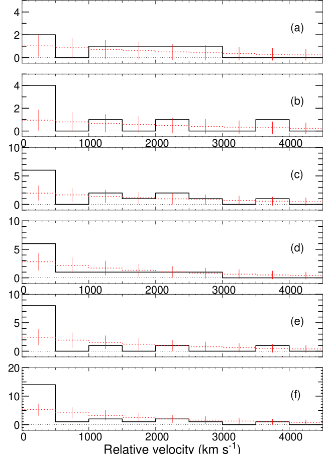
Figure 5: Number of coincidences versus the velocity separation $|\Delta v|$ between the two lines for rest equivalent width threshold of $w_{\rm{r}}>$ 0.3 Å. Panel (a): for pairs with separation $\sim\,$2 arcmin, Q 0037$-$3544 & Q 0037$-$3545 and PC 1320+4755A&B; Panel (b): for pairs with separation $\sim\,$3 arcmin, LBQS 0019$-$0145A&B and Q 0035$-$3518 & Q 0035$-$3520; Panel (c): for the four pairs. Panels (d),(e) and (f) are the same as, respectively, Panels (a), (b) and (c) but after adding data of Young et al. 2001. Dotted lines correspond to the expected number of coincidences from a randomly placed population of lines.

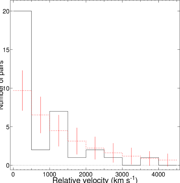
Figure 6: Number of coincidences versus the velocity separation $|\Delta v|$ between the two lines for the complete sample.

From the master line list, we selected lines with $w_{\rm r}>$0.3 Å  and applied the Nearest-Neighbor method as described in e.g. Young et al. (2001) to estimate the level of correlation between absorptions detected along adjacent lines of sight. In this method, there is no a priori velocity separation limit in the definition of a coincidence. A couple of lines along two different lines of sight is declared to be a coincidence if each of the lines is the nearest neighbor of the other. Note that the procedure underestimate the clustering signal as it does not take into account the difference of S/N ratio along the two lines of sight.

The distributions of velocity separations ($|\Delta v|$) between the two lines in a coincidence are plotted in Fig. 5 for the pairs with angular separation $\sim$2 arcmin (Panel a), 3 arcmin (Panel b) and the complete sample (Panel c). To improve statistics, we have added to our results, the data of Young et al. (2001) on two additional pairs separated by $\sim$2 arcmin and $\sim$3 arcmin. The results are plotted in Fig. 5 for the pairs with an angular separation $\sim$2 (Panel d), 3 arcmin (Panel e) and for all the pairs (Panel f).

To estimate the excess of correlation with respect to randomly placed absorption lines, we produced 100000 simulated master line lists drawn from a population of randomly redshifted lines, taking the same number of lines and the same wavelength  range as in the observed spectra. Results of applying the same method to the simulated line lists are given as dotted lines in Fig. 5. The error bars in the figure correspond to the rms of the values found in the simulation. As the corresponding distribution is not Gaussian, we indicate in the following the probability that the observed number of coincidences occurs in the simulated population.

We detect 2 and 4 coincidences with $|\Delta v|$ smaller than 500 km s^-1 in the two pairs separated by $\sim$2 arcmin and $\sim$3 arcmin respectively. The fact that the number of coincidences is smaller in the closest pairs is not statistically significant. When the complete sample is used (Panel c of Fig. 5), the excess in the first bin ($|\Delta v|$$<$500 km s^-1) is significant at the 99.20% level. To increase the statistics, we have added to our sample data from Young et al. (2001). The total number of coincidences with $|\Delta v|$$<$500 km s^-1 and $w_{\rm r}$ $>$ 0.3 Å  is increased to 6, 8 and 14 for the pairs separated by $\sim$2 arcmin, $\sim$3 arcmin and the complete sample. The corresponding excesses relative to simulations of randomly placed lines are significant at the 95.57%, 99.92% and 99.97% levels respectively. The excess is about the same when no threshold is applied to the equivalent width (see Fig. 6). In that case, the number of coincidences in the first bin is 20 and the excess is detected at the 4$\sigma$ level.

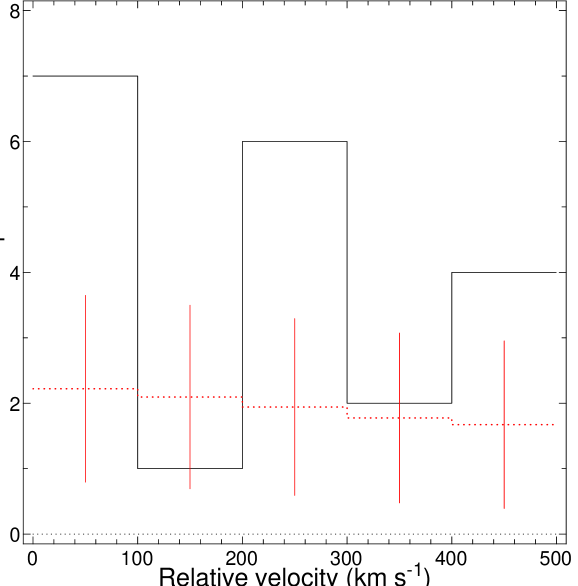
Figure 7: Velocity distribution of the 20 coincidences with $|\Delta v|$ $<$ 500 km s^-1. The dotted line indicates the expected number of coincidences from the Monte-Carlo simulations.

This clearly shows that the Lyman-$\alpha$ forest is correlated on scales larger than 1$\,h^{-1}_{50}$ Mpc proper at $z$ $\sim$ 1. However, we should note that, in the complete sample, 12 of the 20 coincidences with $|\Delta v|$  smaller than 500 km s^-1 actually have $|\Delta v|$ greater than 200 km s^-1. This is also the case for 8 of the 14 coincidences in the $w_{\rm r}$ $>$ 0.3 Å sample. These velocity differences are probably related to peculiar velocities of different objects and reveal that the scale we probe is not related to the real size of individual absorbers.

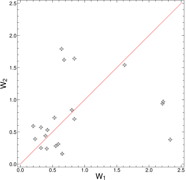
Figure 8: Equivalent width observed along one line of sight versus the one observed along the second line of sight for the 20 coincidences with velocity difference smaller than 500 km s^-1.

In Fig. 8 we plot the equivalent width observed along one line of sight versus the equivalent width observed along the second line of sight for the 20 pairs with velocity differences smaller than 500 km s^-1. There is no clear trend in the plot. This is not really surprizing as we do not expect the absorption strengths to be correlated at such a separation neither in the case of a common absorber nor in the case of independent objects.

6 Conclusion

We have searched for coincidences of Lyman-$\alpha$ absorbers at $z\leavevmode\nobreak\ \leq$ 1 along the lines of sight toward four pairs of quasars with separations 2$-$3 arcmin, observed with HST  STIS. Using the Nearest-Neighbor statistics, we have constructed the distribution of the velocity difference between absorption lines detected along two adjacent lines of sight. We have compared this observed distribution to that derived from Monte-Carlo simulations placing at random the same number of lines in the same wavelength ranges as in the observations. For lines with $w_{\rm r}$ $>$ 0.3 Å , we find an excess of coincidences with velocity separations smaller than 500 km s^-1 significant at the 99.2% level. Combining our data with those in the literature (Young et al. 2001), the excess relative to simulations is significant at the 99.97% level for lines with $w_{\rm r}$ $>$ 0.3 Å  and at the 99.98% level if no condition on the equivalent width is imposed.

The result is consistent with the findings of similar studies at higher redshift (Crotts & Fang 1998, Williger et al. 2000). There is however an important difference between high and intermediate redshift observations. At high redshift, the excess is seen for velocity separations between two coincident lines smaller than 200 km s^-1. At lower redshift, the mean velocity difference is larger (see Fig. 7). This is not a systematic effect related to the low spectral resolution of our data. It could be related to the increase of peculiar velocities with decreasing redshift for comparable spatial scales. This conclusion is strengthened by the fact that the transverse correlation, $\chi\propto\sum_{i}{(1-F_{1}(\lambda_{i}))\times(1-F_{2}(\lambda_{i}))}$ where $F_{1}(\lambda_{i})$ and $F_{2}(\lambda_{i})$ are the two QSO normalized fluxes at wavelength $\lambda_{i}$, at $z$ $\sim$ 1 measured on our spectra is very small, $|\chi|<0.01$, whereas it is of the order of 0.2 at $z$ $\sim$ 2 for the same separation (Rollinde et al. in preparation, see also McDonald 2000, 2001 and Viel et al. 2001). This can be explained by the fact that large values of $\chi$ are due to coincidences with velocity separations smaller than the spectral resolution. In conclusion, evolution from high to low redshift is not seen in the level of correlation but rather in the velocity difference between lines of sight which increases with decreasing redshift. Simulations have shown that absorption lines with a given column density correspond to higher overdensities at low-redshift compared to high redshift and most of the Lyman-$\alpha$ forest at low redshift is to be revealed by very weak lines (Riediger et al. 1998; Theuns et al. 1998; Penton et al. 2000). Therefore, detailed study of the cosmological evolution of the Lyman-$\alpha$ forest will only be possible when the sensitivity of the instruments will be high enough to routinely detect lines with $w_{\rm r}$ $<$ 0.01 Å in the UV.

- (1) Bechtold, J., Crotts, A. P. S., Duncan, R. C., & Fang, Y. 1994, ApJ, 437, L83
- (2) Bergeron, J., Petitjean, P., Sargent, W. L. W., et al. 1994, ApJ, 436, 33
- (3) Boissé, P., Boulade, O., Kunth, D., Tytler, D., & Vigroux, L. 1992, A&A, 262, 401
- (4) Bond, J. R.,& Wadsley, J. W. 1998, eds. P. Petitjean & S. Charlot, XIII IAP Workshop, Editions Frontières, Paris, 143
- (5) Bond, N. A., Churchill, C. W., Charlton, J. C., & Vogt, S. S. 2001, ApJ, 557, 761
- (6) Cen, R., Miralda-Escudé, J., Ostriker, J.P., & Rauch, M. 1994, ApJ, 437, L9
- (7) Charlton, J. C., Anninos, P., Zhang, Y., & Norman, M. L., 1997, ApJ, 485, 26C
- (8) Croft, R. A. C., Weinberg, D. H., Bolte, M., et al. 2000, astro-ph/0012324
- (9) Crotts, A. P. S., & Fang, Y. 1998, ApJ, 502, 16
- (10) Dinshaw, N., Impey, C. D., Foltz, C. B., Weymann, R. J., & Chaffee, F. H. 1994, ApJ, 437, L87
- (11) Dinshaw, N., Foltz, C. B., Impey, C. D., Weymann, R. J., & Morris S. L. 1995, Nature, 373, 223
- (12) Dinshaw, N., Foltz, C. B., Impey, C. D., & Weymann, R. J. 1998, Nature, 494, 567
- (13) D’Odorico, V., Cristiani, S., D’Odorico, S., Fontana, A., Giallongo, E., & Shaver, P. 1998, A&A, 339, 678
- (14) D’Odorico,V., Petitjean, P., & Cristiani, S. 2002, astro-ph/0205299
- (15) Foltz, C. B., Weymann, R. J., Röser, H. J., & Chaffee, F. H. 1984, ApJ, 440, 458
- (16) Hernquist, L., Katz, N., Weinberg, D. H., & Miralda-Escudé, J. 1996, ApJ, 457, L51
- (17) Jannuzi, B. T., Bahcall, J. N., Bergeron, J., et al. 1998, ApJS, 118, 1
- (18) Ledoux, C., Bergeron, J., & Petitjean, P. 2001, A&A accepted, astro-ph/0202134
- (19) Lindler, D.J. 1998, CALSTIS Reference Guide (Version 5.1), http://hires.gsfc.nasa.gov/stis/software/software.html
- (20) McDonald, P. 2000, AAS, 197, 6602M
- (21) McDonald, P. 2001, astro-ph/0108064
- (22) Miralda-Escudé, J., Cen, R., Ostriker, J. P., & Rauch, M. 1996, ApJ, 471, 582
- (23) Monier, E. M., Turnshek, D. A., & Lupie, O. L. 1998, ApJ, 496, 177
- (24) Monier, E. M., Turnshek, D. A., & Hazard, C. 1999, ApJ, 522, 627
- (25) Mücket, J. P., Petitjean, P., Kates, R., & Riediger, R. 1996, A&A, 308, 17
- (26) Penton, S. V., Shull, J. M., & Stocke, J. T. 2000, ApJ, 544, 150
- (27) Petitjean, P. 1997, in ESO Workshop The Early Universe with the VLT ed. J. Bergeron, p. 266
- (28) Petitjean, P., Mücket, J. P., & Kates, R. E. 1995, A&A, 295, L9
- (29) Petitjean, P., Surdej, J., Smette, A., Shaver, P., Mücket, J. P., & Remy, M. 1998, A&A, 334, L45
- (30) Rollinde, E., Petitjean, P., & Pichon, C. 2001, A&A, 376, 28
- (31) Riediger, R., Petitjean, P., & Mücket, J. P. 1998, A&A, 329, 30
- (32) Sargent, W. L. W., Young, P. J., & Schneider, D. P. 1982, ApJ, 256, 374
- (33) Shaver, P. A., Boksenberg, A., & Robertson, J. G. 1982, ApJ, 261, L7
- (34) Shaver, P. A., & Robertson, J. G. 1983, ApJ, 268, L57
- (35) Smette, A., Robertson, J. G., Shaver, P. A., Reimers, D., Wisotzki, L., & Koehler, T. 1995, A&AS, 113, 199
- (36) Smette, A., Surdej, J., Shaver, P. A., Foltz, C. B., Chaffee, F. H., Weymann, R. J., Williams, R. E., & Magain, P. 1992, ApJ, 389, 39S
- (37) Theuns, T., Leonard, A., & Efstathiou, G. 1998, MNRAS, 297, L49
- (38) Viel, M., Matarrese, S., Mo, H. J., Haehnelt, M. G., & Theuns, Tom 2002, MNRAS, 329, 848
- (39) Weymann, R. J., & Foltz, C. B. 1983, ApJ, 272, L1
- (40) Williger, G. M., Hazard, C., Baldwin, J. A., & McMahon, R.G. 1996, ApJS, 104, 145
- (41) Williger, G. M., Smette, A., Hazard, C., Baldwin, J. A., & McMahon, R.G. 2000, ApJ, 532, 77
- (42) Young, P. A., Impey, C. D., & Foltz, C. B. 2001, ApJ, 549, 76
- (43) Zhang, Y., Anninos, P., & Norman, M. L. 1995, ApJ, 453, L57