Determining the Cosmic Distance Scale from Interferometric Measurements of the Sunyaev-Zel’dovich Effect

Abstract

We determine the distances to 18 galaxy clusters with redshifts ranging from $z\sim 0.14$ to $z\sim 0.78$ from a maximum likelihood joint analysis of 30 GHz interferometric Sunyaev-Zel’dovich effect (SZE) and X-ray observations. We model the intracluster medium (ICM) using a spherical isothermal $\beta$ model. We quantify the statistical and systematic uncertainties inherent to these direct distance measurements, and we determine constraints on the Hubble parameter for three different cosmologies. These distances imply a Hubble constant of $60^{+4}_{-4\phantom{0}}\,{}^{+13}_{-18}$ km s^-1 Mpc^-1 for an $\mbox{$\Omega_{M}$}=0.3$, $\mbox{$\Omega_{\Lambda}$}=0.7$ cosmology, where the uncertainties correspond to statistical followed by systematic at 68% confidence. With a sample of 18 clusters, systematic uncertainties clearly dominate. The systematics are observationally approachable and will be addressed in the coming years through the current generation of X-ray satellites (Chandra & XMM-Newton) and radio observatories (OVRO, BIMA, & VLA). Analysis of high redshift clusters detected in future SZE and X-ray surveys will allow a determination of the geometry of the universe from SZE determined distances.

1 Introduction

Analysis of Sunyaev-Zel’dovich effect (SZE) and X-ray data provides a method of directly determining distances to galaxy clusters at any redshift. Clusters of galaxies contain hot ($\mbox{$k_{\mbox{\tiny B}}$}T_{e}\sim 10$ keV) gas, known as the intracluster medium (ICM), trapped in their potential wells. Cosmic microwave background (CMB) photons passing through a massive cluster interact with the energetic ICM electrons with a $\tau\approx 0.01$ probability. This inverse Compton scattering preferentially boosts the energy of a scattered CMB photon causing a small ($\lesssim 1$ mK) distortion in the CMB spectrum, known as the Sunyaev-Zel’dovich effect (Sunyaev & Zel’dovich, 1970, 1972). The SZE appears as a decrement for frequencies $\lesssim 218$ GHz and as an increment for frequencies $\gtrsim 218$ GHz. The SZE is proportional to the pressure integrated along the line of sight $\Delta T\propto\int n_{e}T_{e}d\ell$. X-ray emission from the ICM has a different dependence on the density $S_{\mbox{\tiny X}}\propto\int n_{e}^{2}\mbox{$\Lambda_{e\mbox{\tiny H}}$}d\ell$, where $\Lambda_{e\mbox{\tiny H}}$ is the X-ray cooling function. Taking advantage of the different density dependencies and with some assumptions about the geometry of the cluster, the distance to the cluster may be determined. SZE and X-ray determined distances are independent of the extragalactic distance ladder and provide distances to high redshift galaxy clusters. The promise of direct distances has been one of the primary motivations for SZE observations.

In the last decade, SZE detections have become routine due to advances in both instrumentation and observational strategy. Recent high signal-to-noise ratio detections have been made with single dish observations at radio wavelengths (Birkinshaw & Hughes, 1994; Herbig et al., 1995; Myers et al., 1997; Hughes & Birkinshaw, 1998), millimeter wavelengths (Holzapfel et al., 1997a, b; Pointecouteau et al., 1999, 2001) and submillimeter wavelengths (Lamarre et al., 1998; Komatsu et al., 1999). Interferometric observations at centimeter wavelengths are now routinely producing high quality images of the SZE (Jones et al., 1993; Grainge et al., 1993; Carlstrom et al., 1996, 1998; Saunders et al., 1999; Grainge et al., 2002b; Reese et al., 2000; Grego et al., 2000; Carlstrom et al., 2000; Grego et al., 2001; Jones et al., 2002).

In this paper, we present a maximum likelihood joint analysis of our 30 GHz interferometric SZE observations with archival Röntgen Satellite (ROSAT) X-ray imaging observations. Cluster X-ray temperatures, metallicity, and H I column densities are taken from the literature. The intracluster medium (ICM) is modeled as a spherical isothermal $\beta$ model. We refine the analysis technique described in Reese et al. (2000) and apply it to a sample of 18 clusters for which we determine distances. These distances are then used to measure the Hubble constant. This is the largest homogeneously analyzed sample of SZE clusters with distance determinations thus far. To date, there are about 20 published estimates of $H_{0}$ based on combining X-ray and SZE data for individual clusters (see Birkinshaw, 1999, for a review and compiled distances). Most notably, those results include one sample consisting of 7 nearby ($z<0.1$) galaxy clusters (Mason et al., 2001; Mason, 1999; Myers et al., 1997) and a sample of 5 intermediate redshift ($0.14<z<0.3$) clusters (Jones et al., 2002).

The cluster sample selection for this paper is discussed in §2. The centimeter wave SZE system and interferometric SZE data are described in §3.1. A brief overview the ROSAT X-ray cluster data is given in §3.2. The analysis method, including uncertainty estimation, is outlined in §4 along with the model fitting results. Distances and our determination of the Hubble parameter appear in §5. Sources of possible systematic uncertainties are discussed in §6. Section 7 contains a discussion of the results and future prospects. Throughout this work, the galaxy cluster Cl $0016+16$ ($z=0.546$) will be used as the example cluster to illustrate both the analysis method and general results. All uncertainties are 68.3% confidence unless explicitly stated otherwise.

2 Cluster Sample

The determination the Hubble parameter requires a large sample of galaxy clusters free of selection effects. For example, clusters selected by X-ray surface brightness will preferentially include clusters elongated along the line of sight. A spherical analysis will underestimate the line of sight length of the cluster, causing the derived Hubble parameter to be biased low. In theory, selecting by X-ray luminosity, $L_{\!\mbox{\tiny X}}$, alleviates the selection bias problem. In practice, this is complicated by the fact that X-ray surveys are surface brightness limited; clusters just at the detection limit that are elongated along the line of sight will be detected while clusters just at the detection limit that are instead extended in the plane of the sky will be missed. Staying well above the detection limit of the survey will alleviate this potential pitfall. Observational considerations for cluster sample selection include the declinations of the clusters, the size (redshift) of the cluster, possible radio point sources in the cluster field, and SZE brightness for which we use $L_{\!\mbox{\tiny X}}$ as an indicator. The Owens Valley Radio Observatory (OVRO) and Berkeley-Illinois-Maryland Association (BIMA) interferometers have been used to observe known X-ray clusters with $z\gtrsim 0.14$, declination $\gtrsim-15^{\circ}$, and $L_{x}\gtrsim 5\times 10^{44}\ h_{50}^{-2}$ erg s^-1 (0.3-3.5 keV band for Einstein and 0.1-2.4 keV band for ROSAT). In addition, short, preliminary observations of many clusters are also performed to investigate possible point sources in the field.

The OVRO/BIMA SZE imaging project initially chose targets from the limited number of known X-ray bright clusters. With the publishing of X-ray cluster surveys, the OVRO/BIMA SZE imaging project chose targets from three X-ray catalogs of galaxy clusters: the Einstein Observatory Extended Medium Sensitivity Survey, EMSS (Gioia et al., 1990; Stocke et al., 1991; Gioia & Luppino, 1994; Maccacaro et al., 1994); the ROSAT X-ray Brightest Abell Clusters, XBACs (Ebeling et al., 1996b, a); and the ROSAT Brightest Cluster Sample, BCS (Ebeling et al., 2000a; Crawford et al., 1999; Ebeling et al., 1998, 1997). We have also recently included two more recent ROSAT samples of distant massive clusters to our cluster selection database: the Wide Angle ROSAT Pointed Survey, WARPS (Fairley et al., 2000; Ebeling et al., 2000b; Jones et al., 1998; Scharf et al., 1997); and the MAssive Cluster Survey, MACS (Ebeling et al., 2001). So far, we have high S/N detections in 21 clusters with redshifts $z>0.45$.

The distance calculation requires three data sets: SZE, X-ray imaging, and X-ray spectroscopic data. We have obtained high signal-to-noise detections of the SZE in 45 galaxy clusters. The subsample of these clusters that also have high signal-to-noise X-ray imaging data and published electron temperatures contains 18 galaxy clusters. Table 1 summarizes the redshifts and X-ray luminosities for each galaxy cluster in our sample.

Table 1: Cluster Sample

		$L_{\!\mbox{\tiny X}}$	band
cluster	redshift	($10^{44}h_{50}^{-2}$ erg s-1)	(keV)	references- $z$; $L_{\!\mbox{\tiny X}}$
MS $1137.5+6625$	0.784	05.4	$0.3-3.5$	D99;GL94
MS $0451.6-0305$	0.550	20.0	$0.3-3.5$	GL94;GL94
Cl $0016+16$	0.546	14.6	$0.3-3.5$	DG92;GL94
RX J$1347.5-1145$	0.451	73.0	$0.1-2.4$	S95;S97
Abell 0370	0.374	11.7	$0.1-2.4$	M88;AE99
MS $1358.4+6245$	0.327	10.6	$0.3-3.5$	GL94;GL94
Abell 1995	0.322	13.4	$0.1-2.4$	P00;B00
Abell 0611	0.288	08.6	$0.1-2.4$	C95;B00
Abell 0697	0.282	19.2	$0.1-2.4$	C95;B00,E98
Abell 1835	0.252	32.6	$0.1-2.4$	SR99;B00,E98
Abell 2261	0.224	20.6	$0.1-2.4$	C95;B00
Abell 0773	0.216	12.1	$0.1-2.4$	SR99;B00,E98
Abell 2163	0.202	37.5	$0.1-2.4$	SR99;E96
Abell 0520	0.202	14.5	$0.1-2.4$	GL94;B00,E98
Abell 1689	0.183	20.7	$0.1-2.4$	SR91;E96
Abell 0665	0.182	15.7	$0.1-2.4$	SR91;B00
Abell 2218	0.171	08.2	$0.1-2.4$	L92;B00
Abell 1413	0.142	10.9	$0.1-2.4$	SR99;B00,E98

3 Data

Here we briefly describe the SZE and X-ray observations and data reduction. Table 2 summarizes the observation times for both the SZE and ROSAT observations of each cluster in our sample. The SZE observation times are the total on-source integration times for the interferometric SZE data used in this analysis. The ROSAT observation times are the total livetimes of the pointings used in this analysis.

Table 2: Cluster Data

	Interferometric SZE Data										ROSAT Data
	OVRO (hr)					BIMA (hr)					PSPC	HRI
cluster	1994	1995	1996	1998		1996	1997	1998	2000		(ks)	(ks)
MS1137	$\cdots$	$\cdots$	$\cdots$	$\cdots$		$\cdots$	40	48	$\cdots$		$\cdots$	99.1
MS0451	$\cdots$	$\cdots$	30	$\cdots$		$\cdots$	$\cdots$	$\cdots$	$\cdots$		15.4	45.9
Cl0016	87	13	$\cdots$	$\cdots$		29	8	$\cdots$	$\cdots$		41.6	70.2
R1347	$\cdots$	$\cdots$	$\cdots$	$\cdots$		$\cdots$	$\cdots$	$\cdots$	20.0		$\cdots$	36.1
A370	$\cdots$	$\cdots$	33	$\cdots$		$\cdots$	26	$\cdots$	$\cdots$		$\cdots$	31.9
MS1358	$\cdots$	$\cdots$	9	7		$\cdots$	$\cdots$	70	$\cdots$		22.1	29.2
A1995	$\cdots$	$\cdots$	58	$\cdots$		$\cdots$	$\cdots$	50	$\cdots$		$\cdots$	37.6
A611	$\cdots$	45	12	$\cdots$		$\cdots$	$\cdots$	$\cdots$	$\cdots$		$\cdots$	17.2
A697	$\cdots$	47	$\cdots$	$\cdots$		$\cdots$	$\cdots$	$\cdots$	$\cdots$		$\cdots$	27.8
A1835	$\cdots$	$\cdots$	$\cdots$	$\cdots$		$\cdots$	$\cdots$	27	$\cdots$		8.5	2.8
A2261	$\cdots$	40	$\cdots$	$\cdots$		$\cdots$	$\cdots$	3	$\cdots$		$\cdots$	16.1
A773	57	9	$\cdots$	$\cdots$		5	$\cdots$	18	$\cdots$		$\cdots$	16.5
A2163	$\cdots$	$\cdots$	25	12		2	10	11	$\cdots$		11.7	35.8
A520	$\cdots$	$\cdots$	$\cdots$	7		13	23	20	$\cdots$		4.7	12.6
A1689	$\cdots$	26	$\cdots$	$\cdots$		$\cdots$	16	$\cdots$	$\cdots$		13.5	22.5
A665	$\cdots$	$\cdots$	$\cdots$	$\cdots$		38	24	$\cdots$	$\cdots$		37.0	98.3
A2218	$\cdots$	64	6	$\cdots$		20	12	$\cdots$	$\cdots$		42.5	35.5
A1413	$\cdots$	$\cdots$	$\cdots$	$\cdots$		11	17	$\cdots$	$\cdots$		7.5	18.6

3.1 Interferometric SZE Data

The extremely low systematics of interferometers make them well suited to study the weak SZE signal. A unique feature of interferometers is their ability to separate the diffuse, negative SZE emission from small scale, positive point source emission through the spatial filtering of the interferometer. Interferometers also provide a well defined angular and spectral filter, which is important in the analysis of the SZE data discussed in §4.

3.1.1 Centimeter-Wave System and Observing Strategy

Over the past several summers, we outfitted the Berkeley-Illinois-Maryland Association (BIMA) millimeter array in Hat Creek, California, and the Owens Valley Radio Observatory (OVRO) millimeter array in Big Pine, California, with centimeter wavelength receivers. Our receivers use cooled ($\sim 10$ K) High Electron Mobility Transistor (HEMT) amplifiers (Pospieszalski et al., 1995) operating over 26-36 GHz with characteristic receiver temperatures of $T_{rx}\sim$11-20 K over the 28-30 GHz band used for the observations presented here. When combined with the BIMA or OVRO systems, these receivers obtain typical system temperatures scaled to above the atmosphere of $T_{sys}\sim 35$-$45$ K. Most telescopes are placed in a compact configuration to maximize sensitivity on angular scales subtended by distant clusters ($\sim$ 1′), but telescopes are always placed at longer baselines for simultaneous detection of point sources. Every half hour we observe a bright quasar, commonly called a phase calibrator, for about two minutes to monitor the system phase and gain. The total integration time for each cluster field is given in Table 2 for both OVRO and BIMA.

An interferometer samples the Fourier transform of the sky brightness distribution multiplied by the primary beam rather than the direct image of the sky. The SZE data files include the positions in the Fourier domain, which depend on the arrangement of the telescopes in the array and the declination of the source, the real and imaginary Fourier components, and a measure of the noise in the real and imaginary components. The Fourier conjugate variables to right ascension and declination are commonly called $u$ and $v$, respectively, and the Fourier domain is commonly referred to as the $u$-$v$ plane. The real and imaginary Fourier component pairs as a function of $u$ and $v$ are called visibilities.

The finite size of each telescope dish results in an almost Gaussian response pattern, known as the primary beam. The product of the primary beam and the sky brightness distribution is equivalent to a convolution in the Fourier domain. The primary beams are measured using holography data for both OVRO and BIMA. The main lobe of the primary beams are well fit by a Gaussian with a full width at half maximum (FWHM) of $4\arcmin\!.2$ for OVRO and $6\arcmin\!.6$ for BIMA at 28.5 GHz. However, we use the measured primary beam profiles for our analysis.

The primary beam sets the field of view. The effective resolution, called the synthesized beam, depends on the sampling of the $u$-$v$ plane and is therefore a function of the configuration of the telescopes and the declination of the source. The cluster SZE signal is largest on the shortest baselines (largest angular scales). The shortest possible baseline is set by the diameter of the telescopes, $D$. Thus the system is not sensitive to angular scales larger than about $\lambda/2D$, which is $\sim 2\arcmin\!.8$ for BIMA observations and $\sim 1\arcmin\!.7$ for OVRO observations. The compact configuration used for our observations yields significant SZE signal at these angular scales, but filters out signal on larger angular scales. Because of the spatial filtering by the interferometer, it is necessary to fit models directly to the data in the $u$-$v$ plane, rather than to the deconvolved image.

Interferometers simultaneously measure both the cluster signal and the point sources in the field. The SZE signal is primarily present in the short baseline data while the response of an interferometer to a point source is independent of the baseline. Therefore, observations with a range of baselines allow us to separate the extended cluster emission from point source emission. We show an example of this after first presenting details of deconvolved 30 GHz images (see Jones et al., 1993; Carlstrom et al., 2000, for additional examples).

3.1.2 Data Reduction

The data are reduced using the MIRIAD (Sault et al., 1995) software package at BIMA and using MMA (Scoville et al., 1993) at OVRO. In both cases, data are excised when one telescope is shadowed by another, when cluster data are not straddled by two phase calibrators, when there are anomalous changes in instrumental response between calibrator observations, or when there is spurious correlation. For absolute flux calibration, we use observations of Mars and adopt the brightness temperature from the Rudy (1987) Mars model. For observations not containing Mars, calibrators in those fields are bootstrapped back to the nearest Mars calibration (see Grego et al., 2001 for more details). The observations of the phase calibrators over each summer give us a summer-long calibration of the gains of the BIMA and OVRO interferometers. They both show very little gain variation, changing by less than 1% over a many-hour track, and the average gains remain stable from day to day. In fact, the gains are stable at the $\sim 1$% level over a period of months.

3.1.3 Data Visualization: 30 GHz Images

Here we present deconvolved images of our 30 GHz interferometric observations. However, we stress that these images are made to demonstrate the data quality. The model fitting is performed in the Fourier plane, where the noise characteristics of the data and the spatial filtering of the interferometer are well understood. The SZE and X-ray image overlays of Figure 2 show that the region of the cluster sampled by the interferometric SZE observations and the X-ray observations is similar for the clusters in our sample. In addition, the interferometer measures a range of angular scales, which is not apparent from the images in Figure 2. Images showing examples of our SZE data at varying resolutions appear in Carlstrom et al. (1996) for Cl0016 and Carlstrom et al. (2000) for R1347.

Point sources are identified from SZE images created with DIFMAP (Pearson et al., 1994) using only the long baseline data ($\gtrsim 2000\ \lambda$) and natural weighting ($\sigma^{-2}$ weight). Approximate positions and fluxes for each point source are obtained from this image and used as inputs for the model fitting discussed in §4.2. The data are separated by observatory, frequency, and year to allow for temporal and spectral variability of the point source flux. The positions and fluxes of the detected point sources from the model fitting are summarized in Table 3. Also listed are the corresponding 1.4 GHz fluxes for these sources from the NRAO VLA Sky Survey (NVSS) (Condon et al., 1998) and the 5 GHz and 15 GHz fluxes for sources in the three cluster fields surveyed by Moffet & Birkinshaw (1989). The uncertainty in the positions of the point sources is $\sim\pm 3\arcsec$ at 68.3% confidence based on model fits of point sources described in §4.2. Figure 1 shows the 30 GHz high resolution ($\geq 2000\ \lambda$) maps (color scale) with NVSS 1.4 GHz contours. The color scale wedge above each image shows the range in the map in units of mJy beam^-1. Contours are multiples of twice the NVSS rms (rms $\sim 0.45$ mJy beam^-1). The FWHM of the 30 GHz synthesized beam is shown in the lower left hand corner of each panel and the 45″ FWHM beam of the NVSS survey is shown in the lower right hand corner of each panel. Table 4 summarizes the sensitivity and the FWHM of the synthesized beam of the high resolution maps used to find point sources in each field and shown in Figure 1.

Table 3: Radio Point Sources

	R.A. (J2000)	Dec. (J2000)	$F_{30.0}$	$F_{28.5}$	$F_{15}$	$F_{5}$	$F_{1.4}$
Field	(h   m   s)	(d   ′  ″)	(mJy)	(mJy)	(mJy)	(mJy)	(mJy)
MS1137	$\cdots$	$\cdots$	$\cdots$	$\cdots$	$\cdots$	$\cdots$	$\cdots$
MS0451	$04$ $54$ $22.1$	$-03$ $01$ $25$	$\phantom{0}1.41^{+0.26}_{-0.26}$	$\phantom{0}1.86^{+0.26}_{-0.26}$	$\cdots$	$\cdots$	$\phantom{0}14.9^{+0.7}_{-0.7}$
Cl0016	$00$ $18$ $31.1$	$+16$ $20$ $45$	$\cdots$	$\phantom{0}9.11^{+1.97}_{-1.97}$	$25.0^{+1.5}_{-1.5}$	$84.5^{+1.1}_{-1.1}$	$269.3^{+8.1}_{-8.1}$
R1347	$13$ $47$ $30.7$	$-11$ $45$ $09$	$\cdots$	$10.81^{+0.19}_{-0.19}$	$\cdots$	$\cdots$	$\phantom{0}47.6^{+1.9}_{-1.9}$
A370	$02$ $39$ $55.5$	$-01$ $34$ $06$	$\phantom{0}0.84^{+0.09}_{-0.09}$	$\phantom{0}0.77^{+0.07}_{-0.07}$	$\cdots$	$\cdots$	$\phantom{0}11.7^{+1.1}_{-1.1}$
MS1358	$13$ $59$ $50.6$	$+62$ $31$ $05$	$\cdots$	$\phantom{0}1.61^{+0.17}_{-0.17}$	$\cdots$	$\cdots$	$\cdots$
A1995	$14$ $53$ $00.5$	$+58$ $03$ $19$	$\phantom{0}0.58^{+0.05}_{-0.05}$	$\phantom{0}0.58^{+0.04}_{-0.04}$	$\cdots$	$\cdots$	$\phantom{0}\phantom{0}8.9^{+0.9}_{-0.9}$
A611	$\cdots$	$\cdots$	$\cdots$	$\cdots$	$\cdots$	$\cdots$	$\cdots$
A697	$\cdots$	$\cdots$	$\cdots$	$\cdots$	$\cdots$	$\cdots$	$\cdots$
A1835	$14$ $01$ $02.0$	$+02$ $52$ $42$	$\cdots$	$\phantom{0}2.76^{+0.14}_{-0.14}$	$\cdots$	$\cdots$	$\phantom{0}41.4^{+1.9}_{-1.9}$
	$14$ $01$ $00.5$	$+02$ $51$ $53$	$\cdots$	$\phantom{0}1.16^{+0.15}_{-0.15}$	$\cdots$	$\cdots$	$\cdots$
A2261	$17$ $22$ $17.1$	$+32$ $09$ $14$	$10.10^{+0.24}_{-0.24}$	$10.80^{+0.24}_{-0.24}$	$\cdots$	$\cdots$	$\phantom{0}24.3^{+1.6}_{-1.6}$
A773	$\cdots$	$\cdots$	$\cdots$	$\cdots$	$\cdots$	$\cdots$	$\cdots$
A2163	$16$ $15$ $43.3$	$-06$ $08$ $40$	$\phantom{0}1.44^{+0.12}_{-0.12}$	$\phantom{0}1.44^{+0.08}_{-0.08}$	$\cdots$	$\cdots$	$\cdots$
A520	$04$ $54$ $01.1$	$+02$ $57$ $47$	$\cdots$	$\phantom{0}7.97^{+0.23}_{-0.23}$	$\cdots$	$\cdots$	$\phantom{0}\phantom{0}6.7^{+0.5}_{-0.5}$
	$04$ $54$ $17.0$	$+02$ $55$ $32$	$\cdots$	$\phantom{0}1.01^{+0.10}_{-0.10}$	$\cdots$	$\cdots$	$\phantom{0}15.3^{+1.1}_{-1.1}$
	$04$ $54$ $20.3$	$+02$ $54$ $56$	$\cdots$	$\phantom{0}1.03^{+0.12}_{-0.12}$	$\cdots$	$\cdots$	$\phantom{0}27.8^{+1.6}_{-1.6}$
A1689	$13$ $11$ $31.6$	$-01$ $19$ $33$	$\phantom{0}1.33^{+0.10}_{-0.10}$	$\phantom{0}1.51^{+0.09}_{-0.09}$	$\cdots$	$\cdots$	$\phantom{0}61.0^{+2.5}_{-2.5}$
	$13$ $11$ $30.1$	$-01$ $20$ $37$	$\phantom{0}0.45^{+0.09}_{-0.09}$	$\phantom{0}0.42^{+0.09}_{-0.09}$	$\cdots$	$\cdots$	$\phantom{0}10.9^{+0.6}_{-0.6}$
A665	$08$ $31$ $30.9$	$+65$ $52$ $35$	$\cdots$	$\phantom{0}4.83^{+0.28}_{-0.28}$	$12.7^{+0.3}_{-0.3}$	$25.7^{+1.6}_{-1.6}$	$\phantom{0}31.1^{+1.3}_{-1.3}$
A2218	$16$ $35$ $22.1$	$+66$ $13$ $23$	$\phantom{0}4.29^{+0.21}_{-0.21}$	$\phantom{0}4.43^{+0.20}_{-0.20}$	$\phantom{0}5.0^{+0.6}_{-0.6}$	$\phantom{0}2.8^{+0.2}_{-0.2}$	$\cdots$
	$16$ $35$ $47.7$	$+66$ $14$ $46$	$\phantom{0}1.36^{+0.10}_{-0.10}$	$\phantom{0}1.59^{+0.11}_{-0.11}$	$\phantom{0}2.4^{+0.6}_{-0.6}$	$\phantom{0}3.7^{+0.3}_{-0.3}$	$\phantom{0}18.0^{+1.8}_{-1.8}$
	$16$ $36$ $16.0$	$+66$ $14$ $23$	$\phantom{0}2.41^{+0.29}_{-0.29}$	$\phantom{0}3.13^{+0.30}_{-0.30}$	$\phantom{0}2.0^{+0.5}_{-0.5}$	$\phantom{0}4.2^{+0.1}_{-0.1}$	$\phantom{0}13.3^{+0.6}_{-0.6}$
A1413	$11$ $55$ $08.7$	$+23$ $26$ $17$	$\cdots$	$\phantom{0}2.01^{+0.23}_{-0.23}$	$\cdots$	$\cdots$	$\phantom{0}28.8^{+1.3}_{-1.3}$

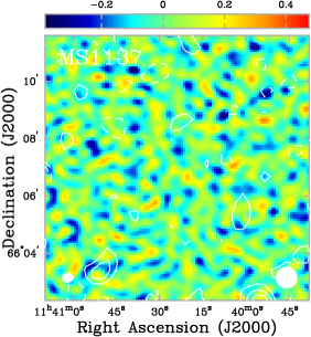
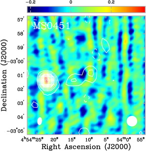
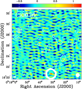
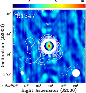
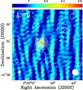
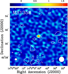
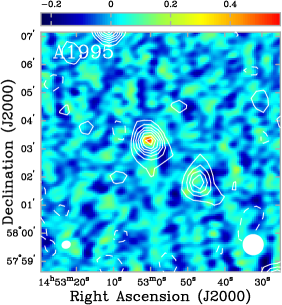
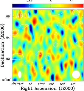
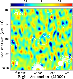
Figure 1: High resolution ($\geq 2000\ \lambda$) 30 GHz (color scale) with NVSS 1.4 GHz contours. The color scale wedge above each image shows the range in the 30 GHz map in units of mJy beam^-1. Contours are multiples of twice the NVSS rms of $\sim 0.45$ mJy beam^-1. The FWHM of the 30 GHz synthesized beam is shown in the lower left hand corner of each panel and the 45″ FWHM beam of the NVSS survey is shown in the lower right hand corner of each panel. The 30 GHz image statistics are summarized in Table 4.
0

–Cont.

Table 4: SZE Image Statistics

	Tapered					High Resolution
		$\sigma$	Beam	$\sigma_{\mbox{\tiny RJ}}$			$\sigma$	Beam
Cluster	Observatory	($\mu$Jy beam-1)	(arcsec)	($\mu$K)		Observatory	($\mu$Jy beam-1)	(arcsec)
MS1137	BIMA	120	$90\times\phantom{0}94$	21		BIMA	105	$20\times 24$
MS0451	OVRO	090	$44\times\phantom{0}69$	45		OVRO	060	$19\times 25$
Cl0016	BIMA	250	$81\times 101$	46		BIMA	220	$14\times 30$
R1347	BIMA	307	$93\times\phantom{0}94$	53		BIMA	245	$17\times 27$
A370	OVRO	060	$56\times\phantom{0}86$	19		OVRO	070	$17\times 23$
MS1358	BIMA	140	$96\times\phantom{0}98$	22		BIMA	120	$17\times 20$
A1995	BIMA	134	$70\times\phantom{0}77$	37		OVRO	065	$17\times 20$
A611	OVRO	060	$48\times\phantom{0}58$	32		OVRO	045	$20\times 39$
A697	OVRO	065	$50\times\phantom{0}53$	37		OVRO	050	$19\times 33$
A1835	BIMA	213	$87\times 121$	30		BIMA	190	$18\times 22$
A2261	OVRO	085	$49\times\phantom{0}53$	49		OVRO	075	$19\times 35$
A773	BIMA	260	$91\times\phantom{0}99$	43		OVRO	090	$19\times 26$
A2163	BIMA	300	$90\times 104$	48		OVRO	085	$19\times 30$
A520	BIMA	180	$90\times 101$	30		OVRO	080	$12\times 16$
A1689	BIMA	320	$93\times\phantom{0}94$	55		OVRO	072	$18\times 49$
A665	BIMA	160	$93\times\phantom{0}99$	26		BIMA	150	$16\times 26$
A2218	BIMA	200	$93\times\phantom{0}99$	31		OVRO	050	$21\times 22$
A1413	BIMA	250	$93\times\phantom{0}99$	44		BIMA	210	$16\times 26$

Figure 2 shows the deconvolved SZE image contours overlaid on the X-ray images for each cluster in our sample. Negative contours are shown as solid lines and the contours are multiples of twice the rms of each image. The images for MS0451 and Cl0016 have been published previously (Reese et al., 2000), but we include them here so that the entire sample appears together. We use DIFMAP (Pearson et al., 1994) to produce the naturally weighted SZE images. If any point sources are detected in the cluster field, they are subtracted from the data and a Gaussian taper applied to the visibilities to emphasize brightness variations on cluster scales before the image is deconvolved (CLEANed). The half-power radius of the Gaussian taper applied varies between 1000 $\lambda$ and 2000 $\lambda$, depending of the observatory and telescope configurations used during the observations. Typically a 1000 $\lambda$ half-power radius taper is applied to BIMA data and a 2000 $\lambda$ half-power radius taper is applied to OVRO data. The full-width at half maximum (FWHM) of the synthesized (restoring) beam is shown in the lower left hand corner of each image. Table 4 summarizes the rms sensitivities and the FWHM’s of the synthesized beams of the tapered maps shown in Figure 2, as well as the corresponding statistics for the high resolution ($\geq 2000\ \lambda$) images. In addition, Table 4 lists the Rayleigh-Jeans (RJ) brightness sensitivities for each tapered, deconvolved image.

3.1.4 Point Source Identification Using Spatial Filtering

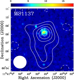
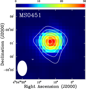
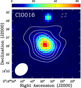
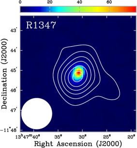
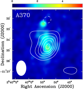
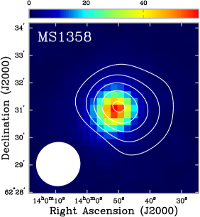
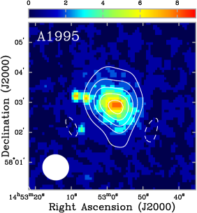
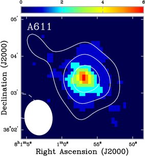
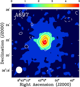
Figure 2: SZE (contours) and X-ray (color scale) images of each cluster in our sample. Negative contours are shown as solid lines. The contours are multiples of 2 $\sigma$ and the FWHM of the synthesized beams are shown in the bottom left corner. The X-ray color scale images are raw counts images smoothed with Gaussians with $\sigma=15$″ for PSPC data and $\sigma=5$″ for HRI data. There is a color scale mapping for the counts above each image. The 30 GHz image statistics are summarized in Table 4.

–Cont.

The identification and removal of point sources by taking advantage of the spatial filtering of the interferometer is illustrated in the panels of Figure 3 for the BIMA SZE Cl0016 data. During the maximum likelihood joint analysis (see §4.2), radio point sources identified from this procedure are modeled and fit for directly in the $u$-$v$ plane. Each panel covers the same angular region, roughly $20\arcmin$ on a side, and each panel shows the FWHM of the synthesized beam in the lower left hand corner. Above each image is the color scale mapping showing the flux density of the map in units of mJy beam^-1. Panel $a$ shows the “natural” image, which includes all of the data. There is smooth, extended, negative emission in the center of the map; this is the SZE decrement of Cl0016. There is also a bright spot roughly 2$\arcmin$ south of the cluster that may be a point source. The large scale symmetric pattern is the synthesized beam of the low resolution data (compare to panel $c$); even when all baselines are considered, the SZE signal dominates. Figure 3$b$ shows the high resolution map using data with projected baselines $\geq 2000\ \lambda$ only. The point source shows up easily now with the characteristic shape of the synthesized beam for these data. We remove the point source by CLEANing. A Gaussian $u$-$v$ taper (half-power radius of 1000 $\lambda$) is then applied to the full data set to emphasize the short baselines, corresponding to the angular scales typical of galaxy clusters, and shown in Figure 3$c$. The cluster is apparent as is the symmetric pattern of the synthesized beam. Deconvolving (CLEANing) the tapered image results in panel $d$, which appeared in Figure 2 overlaid on X-ray data. The contours are multiples of twice the rms of the map.

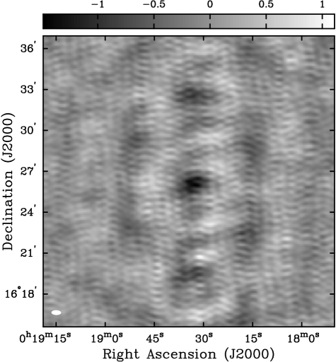
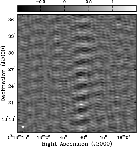
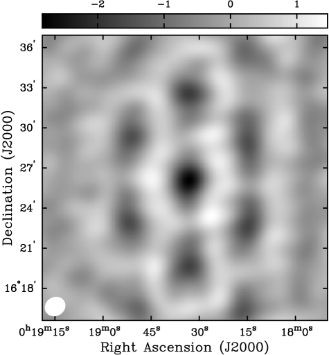
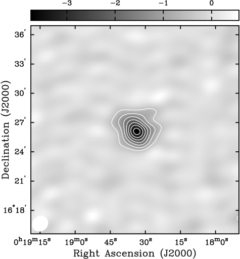
Figure 3: Panels illustrating how the spatial filtering of the interferometer is used to disentangle the point source emission from the SZE emission. Each panel is roughly $20\arcmin$ on a side with the FWHM of the synthesized beam shown in the lower left hand corner. The mapping of the color scale is shown above each panel in units of mJy beam^-1. Panels: $a$) “natural”; $b$) high resolution ($\geq 2000\ \lambda$); $c$) tapered map after point source removal; and $d$) deconvolved SZE image (contours are multiples of 2 $\sigma$). See text for details.                  a)                                                                         b)                  c)                                                                         d)

3.2 ROSAT X-ray Data

We use archival Röntgen Satellite (ROSAT) data from both the Position Sensitive Proportional Counter (PSPC) and High-Resolution Imager (HRI) instruments. The live times of the observations we use are listed in Table 2 for both PSPC and HRI observations.

3.2.1 Data Reduction

We use the Snowden Extended Source Analysis Software (ESAS) (Snowden et al., 1994; Snowden, 1998) to reduce the data. We use the ESAS software to generate a raw counts image, a noncosmic background image, and an exposure map for the HRI (0.1-2.4 keV) data and for each of the Snowden bands R4-R7 (PI channels $52-201$; approximately $0.5-2.0$ keV) for the PSPC data, using a master veto rate (a measure of the cosmic-ray and $\gamma$-ray backgrounds) of 200 counts s^-1 for the PSPC data. We examine the light curve data of both instruments looking for time intervals with anomalously high count rates (short-term enhancements) and for periods of high scattered solar X-ray contamination. Contaminated and anomalously high count rate data are excised. The Snowden software produces $512\times 512$ pixel images with $14.^{\!\!\!\prime\prime}947$ pixels for the PSPC and $5.^{\!\!\!\prime\prime}0$ pixels for the HRI. For the PSPC, final images for all of the R4-R7 bands together are generated by adding the raw counts images and the background images. Each Snowden band has a slightly different effective exposure map and there is an energy dependence in the point spread function (PSF). Thus, we generate a single exposure image and a single PSF image by combining cluster photon-weighted averages of the four exposure images and the four PROS (Worrall et al., 1992; Conroy et al., 1993) generated on-axis PSF images. The cluster photon-weighting is determined using the background subtracted detected photons within a circular region centered on the cluster. The region selected to construct the weights is the largest circular region encompassing the cluster which contains no bright point sources, typically a 15 pixel radius.

3.2.2 X-ray Images and Data Properties

We show smoothed X-ray raw counts images in Figure 2 (color) with SZE image contours overlaid. PSPC images are shown when available and HRI images otherwise. Table 2 summarizes the on-source integration time of the ROSAT observations of the clusters in our sample for both the PSPC and HRI. These images roughly contain a few thousand cluster counts. PSPC images are smoothed with Gaussians with $\sigma=15$″ and HRI images with $\sigma=5$″. The color scale wedge above each figure shows the mapping between color and detector counts.

3.2.3 X-ray Spectral Data

We used published temperatures, metallicities, and H I column densities from observations with the Advanced Satellite for Cosmology and Astrophysics (ASCA). Temperatures and metallicities for most of the clusters in our sample appear in Allen & Fabian (1998a), Allen & Fabian (1998b), and Allen (2000). When there is a detailed account of the analysis for a particular cluster we use those results instead. When fitted metallicities are unavailable, we adopt a 0.2 solar metallicity with a 100% uncertainty. We use fitted H I column densities when available, otherwise those from 21 cm surveys of our galaxy (Dickey & Lockman, 1990) are adopted. We assign a conservative 50% uncertainty to the column densities adopted from 21 cm surveys of our galaxy. Table 5 summarizes our adopted electron temperatures, metallicities, and column densities with references for the sources of this information.

Table 5: X-ray Spectral Information

	$kT_{e}$		$N_{\mbox{\tiny H}}$
cluster	(keV)	[Fe$/$H]	($\times 10^{20}$ cm-2)	ref–$T_{e}$; [Fe$/$H]; $N_{\mbox{\tiny H}}$
MS1137	$\phantom{0}\phantom{0}5.7^{+1.3\phantom{0}}_{-0.7\phantom{0}}$	$0.43^{+0.26}_{-0.24}$	$1.00$	D99;D99;D99
MS0451	$\phantom{0}10.4^{+1.0\phantom{0}}_{-0.8\phantom{0}}$	$0.15^{+0.07}_{-0.07}$	$\phantom{0}3.00^{+0.40}_{-0.30}$	D96;D96;D96
Cl0016	$\phantom{0}7.55^{+0.72}_{-0.58}$	$0.07^{+0.11}_{-0.07}$	$\phantom{0}5.59^{+0.41}_{-0.36}$	HB98;HB98;HB98
R1347	$\phantom{0}\phantom{0}9.3^{+0.7\phantom{0}}_{-0.6\phantom{0}}$	$0.33^{+0.06}_{-0.06}$	$10.00^{+4.00}_{-4.00}$	S97;S97;S97
A370	$\phantom{0}\phantom{0}6.6^{+0.7\phantom{0}}_{-0.5\phantom{0}}$	$0.3^{+0.1}_{-0.1}$	3.1	O98;O98;G
MS1358	$\phantom{0}7.48^{+0.50}_{-0.42}$	$0.32^{+0.09}_{-0.09}$	1.93	AF98;AF98b;G
A1995	$\phantom{0}8.59^{+0.86}_{-0.67}$	$0.14^{+0.07}_{-0.07}$	$\phantom{0}5.0^{+1.6}_{-1.6}$	P00;P00;P00
A611	$\phantom{0}\phantom{0}6.6^{+0.6\phantom{0}}_{-0.6\phantom{0}}$	0.20	4.99	HPC;–;G
A697	$\phantom{0}\phantom{0}9.8^{+0.7\phantom{0}}_{-0.7\phantom{0}}$	0.20	3.41	HPC;–;G
A1835	$\phantom{0}8.21^{+0.19}_{-0.17}$	$0.35^{+0.04}_{-0.03}$	2.32	AF98;AF98b;G
A2261	$\phantom{0}8.82^{+0.37}_{-0.32}$	$0.32^{+0.06}_{-0.05}$	3.28	AF98;AF98b;G
A773	$\phantom{0}9.29^{+0.41}_{-0.36}$	$0.21^{+0.05}_{-0.05}$	1.44	AF98;AF98b;G
A2163	$\phantom{0}12.2^{+1.1\phantom{0}}_{-0.7\phantom{0}}$	$0.40^{+0.09}_{-0.08}$	$16.50^{+0.90}_{-1.14}$	M96;EAB95;EAB95
A520	$\phantom{0}8.33^{+0.46}_{-0.40}$	$0.14^{+0.06}_{-0.06}$	7.80	AF98;AF98b;G
A1689	$\phantom{0}9.66^{+0.22}_{-0.20}$	$0.29^{+0.03}_{-0.03}$	1.82	AF98;AF98b;G
A665	$\phantom{0}9.03^{+0.35}_{-0.31}$	$0.22^{+0.04}_{-0.05}$	4.24	AF98,AF98b;G
A2218	$\phantom{0}7.05^{+0.22}_{-0.21}$	$0.18^{+0.04}_{-0.04}$	3.24	AF98;AF98b;G
A1413	$\phantom{0}7.54^{+0.17}_{-0.16}$	$0.28^{+0.03}_{-0.03}$	2.19	AF98;AF98b;G

Temperatures for many of our clusters also appear in Mushotzky & Scharf (1997). Multiple temperature determinations agree within the 1 $\sigma$ intervals for most of the clusters in our sample. The measurements overlap within $2\ \sigma$ in the worst cases, i.e., for the clusters, MS1358, A1995, A2163, A1689, and A1413. The temperatures, metallicity, column densities, and redshift of the cluster are used to determine the X-ray cooling functions and the conversion factor between detector counts and cgs units, $\Sigma$ (see §3.2.4 below for details). The cooling functions and conversion factors are summarized in Table 6.

Table 6: X-ray Cooling Functions

		PSPC			HRI
cluster	$\Lambda_{e\mbox{\tiny H}0}$	$\Lambda_{e\mbox{\tiny H}0}^{det}$	$\Sigma$		$\Lambda_{e\mbox{\tiny H}0}^{det}$	$\Sigma$	$\frac{\mbox{$n_{e}$}}{\mbox{$n_{\mbox{\tiny H}}$}}=\frac{\mbox{$\mu_{\mbox{\tiny H}}$}}{\mbox{$\mu_{e}$}}$	$\Lambda_{\mbox{\tiny bol}}$
MS1137	7.751	$\cdots$	$\cdots$		1.765	2.461	1.202	2.146
MS0451	6.948	3.263	1.373		1.470	3.050	1.198	2.702
Cl0016	6.922	3.003	1.489		1.289	3.471	1.197	2.260
R1347	6.922	$\cdots$	$\cdots$		1.167	4.089	1.201	2.643
A370	6.790	$\cdots$	$\cdots$		1.627	3.037	1.200	2.223
MS1358	6.717	3.785	1.336		1.793	2.821	1.200	2.371
A1995	6.434	$\cdots$	$\cdots$		1.434	3.395	1.198	2.448
A611	6.511	$\cdots$	$\cdots$		1.489	3.395	1.199	2.175
A697	6.334	$\cdots$	$\cdots$		1.570	3.148	1.199	2.647
A1835	6.462	3.839	1.344		1.775	2.909	1.201	2.496
A2261	6.359	$\cdots$	$\cdots$		1.649	3.150	1.200	2.570
A773	6.171	$\cdots$	$\cdots$		1.870	2.715	1.199	2.581
A2163	6.135	2.555	1.998		1.021	5.000	1.202	3.064
A520	6.119	3.209	1.586		1.337	3.807	1.198	2.411
A1689	6.158	3.899	1.335		1.835	2.836	1.200	2.673
A665	6.102	3.616	1.428		1.570	3.289	1.199	2.550
A2218	6.112	3.789	1.378		1.691	3.086	1.198	2.237
A1413	6.133	4.000	1.343		1.856	2.894	1.200	2.361

3.2.4 X-ray Cooling Function

The X-ray cooling function enters the distance calculation linearly and indirectly as the conversion between detector counts and cgs units (see §4.1). We use a Raymond-Smith (1977) spectrum to describe the hot ICM, which includes contributions from electron-ion thermal bremsstrahlung, line emission, recombination, and two photon processes. We replace the non-relativistic bremsstrahlung calculation in the Raymond-Smith model with the relativistic calculation of Gould (1980). A discussion of this calculation appears in Reese et al. (2000).

The cooling function results for the ROSAT data used in our analysis are summarized in Table 6, where $\Lambda_{e\mbox{\tiny H}0}$ is the cooling function in cgs units, $\Lambda_{e\mbox{\tiny H}0}^{det}$ is the cooling function in detector units, $\Sigma$ is the conversion between counts and cgs units, and $\Lambda_{\mbox{\tiny bol}}$ is the bolometric cooling function. The cooling functions with relativistic corrections are typically 1.05 times the Raymond-Smith “uncorrected” value for the clusters in our sample.

4 Method

4.1 Angular Diameter Distance Calculation

The calculation begins by constructing a model for the cluster gas distribution. We use a spherical isothermal $\beta$ model to describe the ICM. With this model, the cluster’s extent along the line of sight is the same as that in the plane of the sky. This is clearly invalid in the presence of cluster asphericities. Thus cluster geometry introduces an important uncertainty in SZE and X-ray derived distances. In general, clusters are dynamically young, are aspherical, and rarely exhibit projected gas distributions which are circular on the sky (Mohr et al., 1995). We currently cannot disentangle the complicated cluster structure and projection effects, but numerical simulations provide a good base for understanding these difficulties. The effects of asphericity contribute significantly to the distance uncertainty for each cluster, but are not believed to result in any significant bias in the Hubble parameter derived from a large sample of clusters (Sulkanen, 1999).

The spherical isothermal $\beta$ model has the form (Cavaliere & Fusco-Femiano, 1976, 1978)

$$n_{e}({\mathbf{r}})=\mbox{$n_{e0}$}\left(1+\frac{r^{2}}{r_{c}^{2}}\right)^{-3\beta/2},$$ (1)

where $n_{e}$ is the electron number density, $r$ is the radius from the center of the cluster, $r_{c}$ is the core radius of the ICM, and $\beta$ is the power law index. With this model, the SZE signal is

$$\Delta T=f_{(x,T_{e})}\mbox{$T_{\mbox{\tiny CMB}}$}\mbox{$D_{\!\mbox{\tiny A}}$}\!\int\!\!d\zeta\,\mbox{$\sigma_{\mbox{\tiny T}}$}n_{e}\frac{\mbox{$k_{\mbox{\tiny B}}$}T_{e}}{m_{e}c^{2}}=\mbox{$\Delta T_{0}$}\left(1+\frac{\theta^{2}}{\theta_{c}^{2}}\right)^{(1-3\beta)/2},$$ (2)

where $\Delta T$ is the thermodynamic SZE temperature decrement/increment, $f_{(x,T_{e})}$ is the frequency dependence of the SZE with $x=h\nu/k\mbox{$T_{\mbox{\tiny CMB}}$}$, $T_{\mbox{\tiny CMB}}$ (=2.728 K; Fixsen et al., 1996) is the temperature of the CMB radiation, $k_{\mbox{\tiny B}}$ is the Boltzmann constant, $\sigma_{\mbox{\tiny T}}$ is the Thompson cross section, $m_{e}$ is the mass of the electron, $c$ is the speed of light, $\Delta T_{0}$ is the central thermodynamic SZE temperature decrement/increment, $\theta$ is the angular radius in the plane of the sky and $\theta_{c}$ the corresponding angular core radius, and the integration is along the line of sight $\ell=\mbox{$D_{\!\mbox{\tiny A}}$}\zeta$. The frequency dependence of the thermal SZE is

$$f_{(x,T_{e})}=\left(x\frac{e^{x}+1}{e^{x}-1}-4\right)\left(1+\delta_{\mbox{\tiny SZE}}(x,T_{e})\right)$$ (3)

where $\delta_{\mbox{\tiny SZE}}(x,T_{e})$ is the relativistic correction to the frequency dependence. In the non-relativistic and Rayleigh-Jeans (RJ) limits, $f_{(x,T_{e})}\rightarrow-2$. We apply the relativistic corrections $\delta_{\mbox{\tiny SZE}}(x,T_{e})$ to fifth order in $kT_{e}/m_{e}c^{2}$ (Itoh et al., 1998), which agrees with other works (Rephaeli, 1995; Rephaeli & Yankovitch, 1997; Stebbins, 1997; Challinor & Lasenby, 1998; Sazonov & Sunyaev, 1998a, b; Molnar & Birkinshaw, 1999; Dolgov et al., 2001) for clusters with $\mbox{$k_{\mbox{\tiny B}}$}T_{e}\leq 15$ keV, satisfied by all the clusters in our sample. This correction decreases the magnitude of $f_{(x,T_{e})}$ by $\lesssim 5$% (typically 3%) for the clusters considered here.

The X-ray surface brightness is

$$S_{x}=\frac{1}{4\pi(1+z)^{4}}\mbox{$D_{\!\mbox{\tiny A}}$}\!\int\!\!d\zeta\,n_{e}\mbox{$n_{\mbox{\tiny H}}$}\mbox{$\Lambda_{e\mbox{\tiny H}}$}\>\;\!=\mbox{$S_{x0}$}\left(1+\frac{\theta^{2}}{\theta_{c}^{2}}\right)^{(1-6\beta)/2},$$ (4)

where $S_{x}$ is the X-ray surface brightness in cgs units (erg s^-1 cm^-2 arcmin^-2), $z$ is the redshift of the cluster, $n_{\mbox{\tiny H}}$ is the hydrogen number density of the ICM, $\mbox{$\Lambda_{e\mbox{\tiny H}}$}=\mbox{$\Lambda_{e\mbox{\tiny H}}$}(T_{e},\mbox{abundance})$ is the X-ray cooling function of the ICM in the cluster rest frame in cgs units (erg cm³ s^-1) integrated over the redshifted ROSAT band, and $S_{x0}$ is the X-ray surface brightness in cgs units at the center of the cluster. Since the X-ray observations are in instrument counts, we also need the conversion factor between detector counts and cgs units, $\Sigma$ ($\mbox{$S_{x0}$}=S_{x0}^{\mbox{\tiny det}}\Sigma$), discussed in detail in Reese et al. (2000) along with a description of the calculation of $\Lambda_{e\mbox{\tiny H}}$, which includes relativistic corrections (Gould, 1980) to the Raymond & Smith (1977) spectrum. The normalizations, $\Delta T_{0}$ and $S_{x0}$, used in the fit include all of the physical parameters and geometric terms that come from the integration of the $\beta$ model along the line of sight.

One can solve for the angular diameter distance by eliminating $n_{e0}$ (noting that $\mbox{$n_{\mbox{\tiny H}}$}=n_{e}\mu_{e}/\mbox{$\mu_{\mbox{\tiny H}}$}$ where $n_{j}\equiv\rho/\mu_{j}m_{p}$ for species $j$) yielding

$$\mbox{$D_{\!\mbox{\tiny A}}$}=\frac{(\mbox{$\Delta T_{0}$})^{2}}{\mbox{$S_{x0}$}}\left(\frac{m_{e}c^{2}}{\mbox{$k_{\mbox{\tiny B}}$}\mbox{$T_{e0}$}}\right)^{2}\frac{\mbox{$\Lambda_{e\mbox{\tiny H}0}$}\mu_{e}/\mbox{$\mu_{\mbox{\tiny H}}$}}{4\pi^{3/2}\,f_{(x,T_{e})}^{2}\,T_{\mbox{\tiny CMB}}^{2}\,\sigma_{\mbox{\tiny T}}^{2}\,(1+z)^{4}}\frac{1}{\theta_{c}}\left[\frac{\Gamma(\frac{3}{2}\beta)}{\Gamma(\frac{3}{2}\beta-\frac{1}{2})}\right]^{2}\frac{\Gamma(3\beta-\frac{1}{2})}{\Gamma(3\beta)}$$ (5)

where $\Gamma(x)$ is the Gamma function. Similarly, one can eliminate $D_{\!\mbox{\tiny A}}$ instead and solve for the central density $n_{e0}$.

More generally, the angular diameter distance is

$$\mbox{$D_{\!\mbox{\tiny A}}$}=\frac{(\mbox{$\Delta T_{0}$})^{2}}{\mbox{$S_{x0}$}}\left(\frac{m_{e}c^{2}}{\mbox{$k_{\mbox{\tiny B}}$}\mbox{$T_{e0}$}}\right)^{2}\frac{\mbox{$\Lambda_{e\mbox{\tiny H}0}$}\mu_{e}/\mbox{$\mu_{\mbox{\tiny H}}$}}{4\pi\,f_{(x,T_{e})}^{2}\,T_{\mbox{\tiny CMB}}^{2}\,\sigma_{\mbox{\tiny T}}^{2}\,(1+z)^{4}}\frac{1}{\theta_{c}}\frac{\int\left(\frac{\mbox{$n_{e}$}}{\mbox{$n_{e0}$}}\right)^{2}\frac{\mbox{$\Lambda_{e\mbox{\tiny H}}$}}{\mbox{$\Lambda_{e\mbox{\tiny H}0}$}}d\eta\left.\right|_{R=0}}{\left[\int\frac{\mbox{$n_{e}$}}{\mbox{$n_{e0}$}}\frac{\mbox{$T_{e}$}}{\mbox{$T_{e0}$}}d\eta\left.\right|_{R=0}\right]^{2}},$$ (6)

where $\theta_{c}$ is the characteristic angular scale of the galaxy cluster whose exact meaning depends on the ICM model (the core radius for the isothermal $\beta$ model) and $\eta\equiv\zeta/\theta_{c}\equiv\ell/r_{c}$ is the line of sight length in units of the characteristic radius, $r_{c}=\theta_{c}\mbox{$D_{\!\mbox{\tiny A}}$}$. For simplicity in notation, we have assumed that the density and temperature models are normalized at the central value (denoted with 0) though any location for the normalization is allowed. The above integrals are along the central line of sight, denoted as zero projected radius $R=0$. The $\Gamma$ functions and the factor of $\pi^{1/2}$ in equation (5) come from the integration of the $\beta$ model along the central line of sight for both the SZE and X-ray models.

4.2 Joint SZE and X-ray Model Fitting

The SZE and X-ray emission both depend on the properties of the ICM, so a joint fit to the interferometric SZE data and the PSPC and HRI X-ray data provides the best constraints on those properties. Each data set is assigned a collection of parameterized models. Typically, SZE data sets are assigned a $\beta$ model and point sources and X-ray images are assigned a $\beta$ model and a cosmic X-ray background model. This set of models is combined for each data set to create a composite model which is then compared to the data.

Our analysis procedure is described in detail in Reese et al. (2000). The philosophy behind the analysis is to keep the data in a reduced but “raw” state and run the model through the observing strategy to compare directly with the data. In particular, the interferometric SZE observations provide constraints in the Fourier ($u$-$v$) plane, so we perform our model fitting in the $u$-$v$ plane, where the noise properties of the data and the spatial filtering of the interferometer are well defined. The SZE model is generated in the image plane, multiplied by the primary beam, and fast Fourier transformed to produce model visibilities. We then interpolate the model visibilities to the $u$ and $v$ of each data visibility and compute the Gaussian likelihood. For X-ray data, the model is convolved with the appropriate point spread function and the Poisson likelihood is computed pixel by pixel, ignoring the masked point source regions.

Each data set is independent, and likelihoods from each data set can simply be multiplied together to construct the joint likelihood. Likelihood ratio tests can then be performed to get confidence regions or compare two models. Rather than working directly with likelihoods, $\mathcal{L}$, we work with $S\equiv-2\ln(\mathcal{L})$. We then construct a $\Delta\chi^{2}$-like statistic from the log likelihoods, $\Delta S\equiv S_{n}-S_{min}$ where $S_{min}$ is the minimum of the $S$ function and $S_{n}$ is the $S$ statistic where $n$ parameters differ from the parameters at $S_{min}$. The statistic $\Delta S$ is sometimes referred to as the Cash (1979) statistic and tends to a $\chi^{2}$ distribution with $n$ degrees of freedom for large $n$ (Kendall & Stuart, 1979, for example). This $\Delta S$ statistic is equivalent to the likelihood ratio test and is used to generate confidence regions and confidence intervals. For one interesting parameter, the 68.3% ($\sim 1\sigma$) confidence level corresponds to $\Delta S=1.0$.

4.2.1 Model Fitting Uncertainty Estimation

Uncertainties in the angular diameter distance from the fit parameters are calculated by varying the interesting parameters to explore the $\Delta S$ likelihood space. The most important parameters in this calculation are $\Delta T_{0}$, $S_{x0}$, $\beta$, and $\theta_{c}$. Radio point sources and the cosmic X-ray background affect $\Delta T_{0}$ and $S_{x0}$, respectively. As a compromise between precision and computation time, we systematically vary $\Delta T_{0}$, $S_{x0}$, $\beta$, and $\theta_{c}$ allowing the X-ray backgrounds for the PSPC and HRI to float independently while fixing the positions of the cluster (both SZE and X-ray), and the positions and flux densities of any radio point sources in the SZE cluster fields. We describe our estimation of the effects of point sources below.

From this four dimensional $\Delta S$ hyper-surface, we construct confidence intervals for each parameter individually as well as confidence intervals for $D_{\!\mbox{\tiny A}}$ due to $S_{x0}$, $\Delta T_{0}$, $\beta$, and $\theta_{c}$ jointly. To compute the 68.3% confidence region we find the minimum and maximum values of the parameter within a $\Delta S$ of 1.0. We emphasize that these uncertainties are meaningful only within the context of the spherical isothermal $\beta$ model.

Measured Radio Point Sources

Two methods of estimating the effect of the measured radio point sources in the cluster field are examined, one which is reasonably quick and one that is more rigorous. For the quick estimate, we first determine the 1 $\sigma$ confidence limits on the flux density of each point source by varying the point source flux density while keeping the ICM parameters fixed at their best fit values. These are the uncertainties listed in Table 3, after correcting for the primary beam attenuation appropriate for each point source’s distance from the pointing center. We then determine the change in the central decrement over the 68.3% confidence region for the point source flux densities by fixing the point source flux density at the $\pm 1\ \sigma$ values and varying $\Delta T_{0}$ while fixing the ICM shape parameters at their best fit values. This is done for each point source in the field and all combinations of the $\pm 1\ \sigma$ flux densities for fields with multiple point sources. We adopt the maximum percentage change in $\Delta T_{0}$ as our uncertainty from radio point sources on the central decrement. The above procedure will be referred to as the quick estimate of the effects of measured radio point sources. We tested this estimate against marginalizing over the point source flux density by varying $\theta_{c}$, $\beta$, $S_{x0}$, $\Delta T_{0}$, and point source flux for each point source, while fixing the X-ray background (simply saves computation time by isolating the point source flux issue). From the marginalized likelihood function we find the best fit and 68.3% uncertainty on $\Delta T_{0}$ and $D_{\!\mbox{\tiny A}}$. The uncertainty from measured radio point sources, $\sigma_{pt}$, is computed assuming the uncertainties add in quadrature from

$$\sigma_{pt}^{2}=\sigma_{mar}^{2}-\sigma_{fix}^{2},$$ (7)

where $\sigma_{mar}$ and $\sigma_{fix}$ are the uncertainties from the marginalized grids and the initial, point source fixed grids, respectively. Marginalizing over point source flux density was performed on two clusters with one point source each, A2261 and MS1358, and one cluster with two point sources, A1835. The quick estimation of the effects of point sources agrees to within 2% on $D_{\!\mbox{\tiny A}}$ (1% on $\Delta T_{0}$) with the marginalized likelihood analysis, just slightly over estimating the uncertainty due to point sources. The marginalization procedure is computationally intensive. Therefore, to save computation time, we use the quick procedure to estimate the effects of detected point sources on the central decrement.

As an additional test, we explore the maximum likelihood parameter space (varying $\theta_{c}$, $\beta$, $S_{x0}$, and $\Delta T_{0}$) with the point source fluxes fixed at the $\pm 1\ \sigma$ values for our three test case clusters: A2261, MS1358, and A1835. The effects of point sources on the central decrement from this study agree within a few percent with both the quick and marginalized procedures. This is what was originally done for MS0451 and Cl0016 (Reese et al., 2000), which is now shown to give essentially the same result as marginalizing over the point source flux. For all clusters, we use the updated, quick estimates of the effects of measured point sources.

4.3 Model Fitting Results

We apply the analysis procedure described above to all 18 of our galaxy clusters. The results from our maximum likelihood joint fit to the SZE and X-ray data are summarized in Table 7, which shows the best-fit ICM shape parameters and the uncertainties on each parameter from the model fit.

So far, we have only shown the SZE data in the form of images though the data are recorded as visibilities. Figure 4 shows the SZE $u$-$v$ radial profiles for Cl0016 with a series of 3 panels illustrating the features of such profiles. These profiles are azimuthal averages in the Fourier plane plotted as a function of the radius in the $u$-$v$ plane, $\sqrt{u^{2}+v^{2}}$. The data are the points with error bars and the best fit $\beta$ model from the joint SZE and X-ray analysis is the solid line averaged the same way as the data. The point sources are subtracted directly from the visibilities before constructing the $u$-$v$ radial profiles. All of these panels are shown on the same scale for easy comparison. Also plotted are the residuals in units of the standard deviation, $\Delta V/\sigma$=(data $-$ model)/$\sigma$. For a circular cluster at the phase center (coincident with the pointing center), one expects a monotonic real component and a zero imaginary component. Clusters are rarely exactly centered at the phase/pointing center of our observations. Therefore, we shift the phase center to the cluster center before constructing the $u$-$v$ radial profiles. The phase shifted radial profiles are shown in the upper panel of Figure 4 for both the real (left) and imaginary (right) components of the complex visibilities. The model provides a good fit to the data for a wide range of spatial frequencies. The middle panel shows the $u$-$v$ radial profile when the phase center is not shifted to the center of the cluster. The off-center cluster introduces corrugation in the Fourier plane modifying the expected real component and introducing a non-zero imaginary component. In addition, asymmetry in the cluster will manifest itself as a non-zero imaginary component. Our model is symmetric and its imaginary component should be identically zero. The attenuation from the primary beam introduces asymmetry, producing a non-zero imaginary component. This is illustrated in the lower panel of Figure 4 showing the $u$-$v$ radial profile including the phase center shift but not including the primary beam correction when computing the model. Notice the model is identically zero unlike the upper panel, where the asymmetry produced by the primary beam on the off-center cluster shows a small imaginary component.

Table 7: ICM Parameters

		$\theta_{c}$	$S_{x0}^{det}$	$S_{x0}$	$\Delta T_{0}$	$D_{\!\mbox{\tiny A}}$
Cluster	$\beta$	(arcsec)	(detector)	(cgs)	($\mu$K)	(Mpc)
MS1137	$0.786^{+0.220}_{-0.120}$	$\phantom{0}19.4^{+6.4}_{-4.0}$	$1.80^{+0.30}_{-0.24}$ $\times 10^{-2}$	$4.43^{+0.74}_{-0.59}$ $\times 10^{-13}$	$-\phantom{0}818^{+98\phantom{0}}_{-113}$	$3179^{+1103}_{-1640}$
MS0451	$0.806^{+0.052}_{-0.043}$	$\phantom{0}34.7^{+3.9}_{-3.5}$	$6.96^{+0.63}_{-0.61}$ $\times 10^{-2}$	$9.56^{+0.86}_{-0.84}$ $\times 10^{-13}$	$-1431^{+98\phantom{0}}_{-93\phantom{0}}$	$1278^{+265\phantom{0}}_{-299\phantom{0}}$
Cl0016	$0.749^{+0.024}_{-0.018}$	$\phantom{0}42.3^{+2.4}_{-2.0}$	$4.14^{+0.15}_{-0.19}$ $\times 10^{-2}$	$6.17^{+0.22}_{-0.28}$ $\times 10^{-13}$	$-1242^{+105}_{-105}$	$2041^{+484\phantom{0}}_{-514\phantom{0}}$
R1347	$0.604^{+0.011}_{-0.012}$	$\phantom{0}\phantom{0}9.0^{+0.5}_{-0.5}$	$6.70^{+0.39}_{-0.34}$ $\times 10^{-1}$	$2.74^{+0.16}_{-0.14}$ $\times 10^{-11}$	$-3950^{+350}_{-350}$	$1221^{+368\phantom{0}}_{-343\phantom{0}}$
A370	$0.518^{+0.090}_{-0.080}$	$\phantom{0}39.5^{+10.5}_{-10.5}$	$8.88^{+1.41}_{-0.99}$ $\times 10^{-3}$	$2.70^{+0.43}_{-0.30}$ $\times 10^{-13}$	$-1253^{+218}_{-533}$	$4352^{+1388}_{-1245}$
MS1358	$0.622^{+0.015}_{-0.015}$	$\phantom{0}18.2^{+1.4}_{-1.5}$	$1.27^{+0.11}_{-0.08}$ $\times 10^{-1}$	$1.70^{+0.15}_{-0.11}$ $\times 10^{-12}$	$-\phantom{0}784^{+90\phantom{0}}_{-90\phantom{0}}$	$\phantom{0}866^{+248\phantom{0}}_{-310\phantom{0}}$
A1995	$0.770^{+0.117}_{-0.063}$	$\phantom{0}38.9^{+6.9}_{-4.3}$	$3.18^{+0.24}_{-0.21}$ $\times 10^{-2}$	$1.08^{+0.08}_{-0.07}$ $\times 10^{-12}$	$-1023^{+83\phantom{0}}_{-77\phantom{0}}$	$1119^{+247\phantom{0}}_{-282\phantom{0}}$
A611	$0.565^{+0.050}_{-0.040}$	$\phantom{0}17.5^{+3.5}_{-3.5}$	$5.91^{+1.06}_{-0.76}$ $\times 10^{-2}$	$2.01^{+0.36}_{-0.26}$ $\times 10^{-12}$	$-\phantom{0}853^{+120}_{-140}$	$\phantom{0}995^{+325\phantom{0}}_{-293\phantom{0}}$
A697	$0.540^{+0.045}_{-0.035}$	$\phantom{0}37.8^{+5.6}_{-4.0}$	$3.24^{+0.22}_{-0.25}$ $\times 10^{-2}$	$1.02^{+0.07}_{-0.08}$ $\times 10^{-12}$	$-1410^{+160}_{-180}$	$\phantom{0}998^{+298\phantom{0}}_{-250\phantom{0}}$
A1835	$0.595^{+0.007}_{-0.005}$	$\phantom{0}12.2^{+0.6}_{-0.5}$	$1.50^{+0.10}_{-0.07}$ $\times 10^{-0}$	$2.02^{+0.14}_{-0.10}$ $\times 10^{-11}$	$-2502^{+150}_{-175}$	$1027^{+194\phantom{0}}_{-198\phantom{0}}$
A2261	$0.516^{+0.014}_{-0.013}$	$\phantom{0}15.7^{+1.2}_{-1.1}$	$1.37^{+0.08}_{-0.08}$ $\times 10^{-1}$	$4.31^{+0.26}_{-0.26}$ $\times 10^{-12}$	$-1697^{+200}_{-200}$	$1049^{+306\phantom{0}}_{-272\phantom{0}}$
A773	$0.597^{+0.064}_{-0.032}$	$\phantom{0}45.0^{+7.0}_{-5.0}$	$3.05^{+0.24}_{-0.24}$ $\times 10^{-2}$	$8.28^{+0.65}_{-0.65}$ $\times 10^{-13}$	$-1260^{+160}_{-160}$	$1450^{+361\phantom{0}}_{-332\phantom{0}}$
A2163	$0.674^{+0.011}_{-0.008}$	$\phantom{0}87.5^{+2.5}_{-2.0}$	$6.82^{+0.15}_{-0.15}$ $\times 10^{-2}$	$1.36^{+0.03}_{-0.03}$ $\times 10^{-12}$	$-1900^{+140}_{-140}$	$\phantom{0}828^{+181\phantom{0}}_{-205\phantom{0}}$
A520	$0.844^{+0.040}_{-0.040}$	$123.3^{+8.0}_{-8.0}$	$2.57^{+0.11}_{-0.11}$ $\times 10^{-2}$	$4.08^{+0.18}_{-0.18}$ $\times 10^{-13}$	$-\phantom{0}662^{+95\phantom{0}}_{-95\phantom{0}}$	$\phantom{0}723^{+270\phantom{0}}_{-236\phantom{0}}$
A1689	$0.609^{+0.005}_{-0.005}$	$\phantom{0}26.6^{+0.7}_{-0.7}$	$4.50^{+0.13}_{-0.11}$ $\times 10^{-1}$	$6.01^{+0.18}_{-0.15}$ $\times 10^{-12}$	$-1729^{+105}_{-120}$	$\phantom{0}688^{+172\phantom{0}}_{-163\phantom{0}}$
A665	$0.615^{+0.006}_{-0.006}$	$\phantom{0}71.7^{+1.5}_{-1.5}$	$4.75^{+0.08}_{-0.08}$ $\times 10^{-2}$	$6.78^{+0.12}_{-0.12}$ $\times 10^{-13}$	$-\phantom{0}728^{+150}_{-150}$	$\phantom{0}466^{+217\phantom{0}}_{-179\phantom{0}}$
A2218	$0.692^{+0.008}_{-0.008}$	$\phantom{0}67.5^{+1.5}_{-1.8}$	$5.14^{+0.12}_{-0.10}$ $\times 10^{-2}$	$7.08^{+0.16}_{-0.14}$ $\times 10^{-13}$	$-\phantom{0}731^{+125}_{-100}$	$1029^{+339\phantom{0}}_{-352\phantom{0}}$
A1413	$0.639^{+0.009}_{-0.009}$	$\phantom{0}47.7^{+2.0}_{-2.0}$	$1.52^{+0.07}_{-0.07}$ $\times 10^{-1}$	$2.04^{+0.09}_{-0.09}$ $\times 10^{-12}$	$-\phantom{0}856^{+110}_{-110}$	$\phantom{0}573^{+171\phantom{0}}_{-151\phantom{0}}$

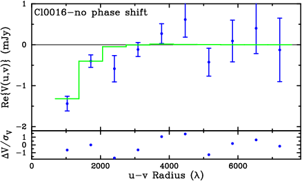
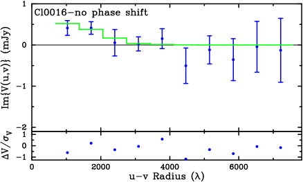
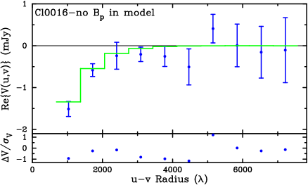
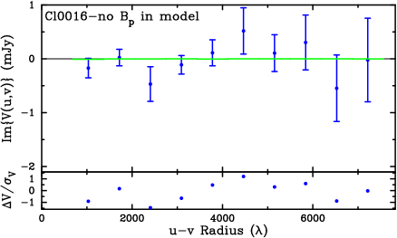
Figure 4: The real and imaginary components of the complex visibilities plotted as a function of radius in the $u$-$v$ plane for Cl0016. The points with error bars are the data and the best fit model from the joint SZE and X-ray analysis is the solid line, averaged the same way as the data. Residuals are shown in units of the standard deviation. Shown are the phase shifted and primary beam corrected (upper panel), not phase shifted (middle panel), and not corrected for primary beam (lower panel) versions. Not shifting the phase center to the center of the cluster (middle panel) shows an imaginary component from this offset. Not applying the primary beam attenuation to the model after shifting the phase to the center of the cluster (lower panel) shows the expected zero imaginary component; a real and symmetric image should have a real only Fourier transform. The asymmetry induced by the primary beam correction for the off-center cluster introduces a small imaginary component (see upper panel).

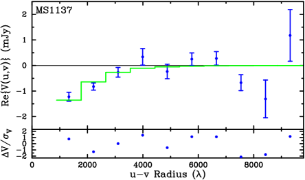
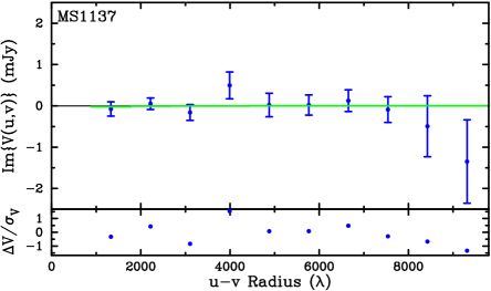
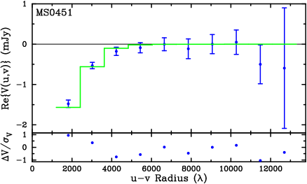
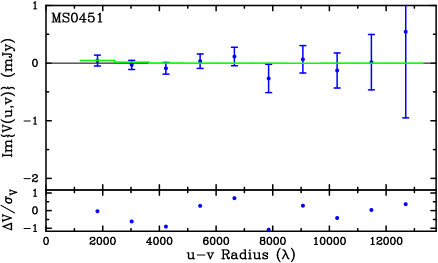
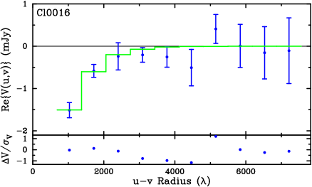
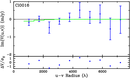
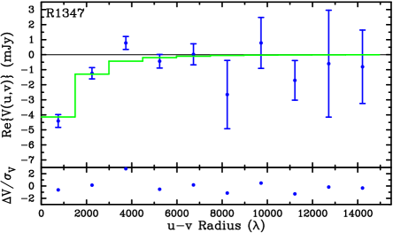
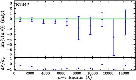
Figure 5: The real and imaginary components of the complex visibilities plotted as a function of radius in the $u$-$v$-plane. The points and error bars are the data and the solid line is the best fit model. Residuals are shown in units of the standard deviation. Any point sources in the cluster field have been subtracted directly from the visibilities and the phase center of the map has been shifted to the center of the cluster before making these radial averages. Non-zero signal in the imaginary components is due to the asymmetry in the cluster and the possible asymmetry introduced by the primary beam correction. The models provide good fits to the data for all the clusters in our sample.

–Cont.

–Cont.

–Cont.

–Cont.

The $u$-$v$ radial profiles for the real and imaginary components of the complex visibilities for each cluster in our sample are shown in Figure 5. Any point sources in the field are subtracted directly from the visibilities and the phase center is shifted to the center of the cluster before azimuthally averaging the real and imaginary components of the complex visibilities. The points with error bars are the data and the best fit model from the joint SZE and X-ray analysis is shown as a solid line, averaged the same way as the data. Also shown are the residuals in units of the standard deviation. A simple $\chi^{2}$ analysis of the SZE $u$-$v$ radial profiles reveals that the models provide a good fit to the data for every cluster. The real and imaginary components are shown on the same scale for each cluster for easy comparison, though the scale on the residuals may change. The cluster with the most apparent imaginary component, A520, is also the cluster with its best fit center the furthest away from the pointing center, $\sim 65\arcsec$. The primary beam attenuation introduces asymmetry and produces a non-zero imaginary component paralleled in the best fit model for A520.

Figure 6 shows the X-ray radial surface brightness profiles and the best fit composite models for each cluster in the sample. Residuals in units of the standard deviation are also plotted, $\Delta S_{x}/\sigma_{S_{x}}$. A simple $\chi^{2}$ analysis of the radial profiles shows that, in general, the models provide a reasonable fit to the data over a large range of angular radii. There are 3 clusters with residuals $\gtrsim 5\ \sigma$ in a few of the radial bins; A1835, A665, and A2281. In A1835 the model systematically underpredicts the surface brightness for a few intermediate radial bins. This cluster contains a strong cooling flow (e.g., Peres et al., 1998), though shows no sign of a central emission excess over the best fit model. The other cooling flow clusters in our sample (see §6.1) do not exhibit large residuals in the X-ray model fit. Both A665 (Gómez et al., 2000; Kalloglyan et al., 1990; Geller & Beers, 1982) and A2218 (Cannon et al., 1999; Girardi et al., 1997; Markevitch, 1997; Kneib et al., 1995) exhibit complicated structure, possibly indicating a recent merger. Though the worst cases, the best fit models for these 3 clusters still provide reasonable descriptions of the data. The only cluster that shows a marginally significant central X-ray surface brightness excess is A2218, which has not been identified with a cooling flow. We also note that the cooling flow clusters in our sample do not exhibit the largest residuals.

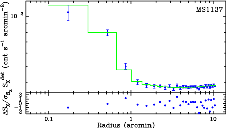
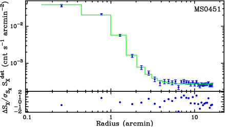
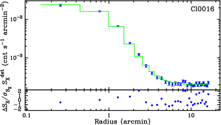
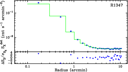
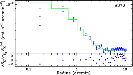
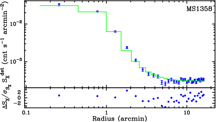
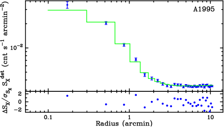
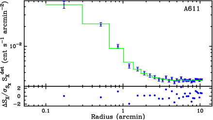
Figure 6: X-ray surface brightness radial profiles with the best fit model and residuals in units of the standard deviation. In general, the models provide good fits to the data over a large range of radii.

–Cont.

–Cont.

5 Distances and the Hubble Constant

We use the results from the maximum likelihood model fitting described in §4.2 and §4.3 to compute the angular diameter distance to each of our 18 galaxy clusters. Table 7 shows the derived angular diameter distances for each galaxy cluster as well as the best fit ICM shape parameters. The uncertainties on $D_{\!\mbox{\tiny A}}$ include the entire observational uncertainty budget, which are shown for each cluster in Table 8. The uncertainties in the fitted parameters come from the procedure described in §4.2.1.

Table 8: $D_{\!\mbox{\tiny A}}$ Observational Uncertainty Budget (percent)

Cluster	Fit	$T_{e}$	$\mbox{$\Lambda_{e\mbox{\tiny H}}$}(Z)$	$\mbox{$\Lambda_{e\mbox{\tiny H}}$}(\mbox{$N_{\mbox{\tiny H}}$})$	$\mbox{$\Lambda_{e\mbox{\tiny H}}$}(T_{e})$	pt src	Total
MS1137	${}^{+22.3}_{-22.9}$	${}^{+24.6}_{-45.6}$	${}^{+4.9}_{-4.7}$	${}^{+\phantom{0}9.0}_{-\phantom{0}6.1}$	${}^{+0.0}_{-0.8}$	${}^{+\phantom{0}0.0}_{-\phantom{0}0.0}$	${}^{+34.7}_{-51.6}$
MS0451	${}^{+13.8}_{-13.1}$	${}^{+15.4}_{-19.2}$	${}^{+1.0}_{-1.0}$	${}^{+\phantom{0}0.9}_{-\phantom{0}1.2}$	${}^{+0.4}_{-0.5}$	${}^{+\phantom{0}0.6}_{-\phantom{0}0.6}$	${}^{+20.7}_{-23.4}$
CL0016	${}^{+17.8}_{-16.4}$	${}^{+15.4}_{-19.1}$	${}^{+1.9}_{-1.2}$	${}^{+\phantom{0}1.1}_{-\phantom{0}1.2}$	${}^{+0.1}_{-0.2}$	${}^{+\phantom{0}1.0}_{-\phantom{0}0.6}$	${}^{+23.7}_{-25.2}$
R1347	${}^{+19.2}_{-17.1}$	${}^{+12.9}_{-15.1}$	${}^{+1.0}_{-1.0}$	${}^{+15.7}_{-11.7}$	${}^{+0.4}_{-0.5}$	${}^{+11.2}_{-11.4}$	${}^{+30.1}_{-28.1}$
A370	${}^{+24.4}_{-16.7}$	${}^{+15.2}_{-21.2}$	${}^{+1.9}_{-1.9}$	${}^{+13.1}_{-\phantom{0}8.2}$	${}^{+0.4}_{-0.6}$	${}^{+\phantom{0}4.0}_{-\phantom{0}4.0}$	${}^{+31.9}_{-28.6}$
MS1358	${}^{+24.0}_{-21.3}$	${}^{+11.2}_{-13.4}$	${}^{+1.5}_{-1.5}$	${}^{+\phantom{0}3.1}_{-\phantom{0}3.0}$	${}^{+0.3}_{-0.4}$	${}^{+10.0}_{-25.2}$	${}^{+28.6}_{-35.8}$
A1995	${}^{+10.3}_{-11.5}$	${}^{+15.6}_{-20.0}$	${}^{+1.1}_{-1.1}$	${}^{+\phantom{0}8.5}_{-\phantom{0}6.5}$	${}^{+0.5}_{-0.7}$	${}^{+\phantom{0}8.2}_{-\phantom{0}7.8}$	${}^{+22.1}_{-25.2}$
A611	${}^{+22.2}_{-20.5}$	${}^{+18.2}_{-18.2}$	${}^{+3.7}_{-3.7}$	${}^{+15.3}_{-\phantom{0}9.8}$	${}^{+0.4}_{-0.5}$	${}^{+\phantom{0}0.0}_{-\phantom{0}0.0}$	${}^{+32.7}_{-29.4}$
A697	${}^{+22.7}_{-18.7}$	${}^{+14.3}_{-14.3}$	${}^{+3.0}_{-3.0}$	${}^{+12.9}_{-\phantom{0}8.2}$	${}^{+0.7}_{-0.7}$	${}^{+\phantom{0}0.0}_{-\phantom{0}0.0}$	${}^{+29.9}_{-25.1}$
A1835	${}^{+13.2}_{-12.6}$	${}^{+\phantom{0}4.1}_{-\phantom{0}4.6}$	${}^{+0.7}_{-0.5}$	${}^{+\phantom{0}3.7}_{-\phantom{0}3.5}$	${}^{+0.2}_{-0.2}$	${}^{+12.4}_{-13.4}$	${}^{+18.9}_{-19.3}$
A2261	${}^{+25.0}_{-22.9}$	${}^{+\phantom{0}7.3}_{-\phantom{0}8.4}$	${}^{+0.9}_{-0.8}$	${}^{+12.7}_{-\phantom{0}8.1}$	${}^{+0.4}_{-0.5}$	${}^{+\phantom{0}3.4}_{-\phantom{0}3.4}$	${}^{+29.2}_{-25.9}$
A773	${}^{+21.8}_{-20.2}$	${}^{+\phantom{0}7.8}_{-\phantom{0}8.8}$	${}^{+0.7}_{-0.7}$	${}^{+\phantom{0}9.3}_{-\phantom{0}6.2}$	${}^{+0.5}_{-0.5}$	${}^{+\phantom{0}0.0}_{-\phantom{0}0.0}$	${}^{+24.9}_{-22.9}$
A2163	${}^{+16.3}_{-14.4}$	${}^{+11.5}_{-18.0}$	${}^{+1.2}_{-1.1}$	${}^{+\phantom{0}2.9}_{-\phantom{0}2.2}$	${}^{+0.7}_{-1.0}$	${}^{+\phantom{0}8.4}_{-\phantom{0}8.6}$	${}^{+21.8}_{-24.8}$
A520	${}^{+32.4}_{-27.2}$	${}^{+\phantom{0}9.6}_{-11.0}$	${}^{+1.0}_{-1.0}$	${}^{+12.1}_{-10.2}$	${}^{+0.3}_{-0.4}$	${}^{+10.2}_{-10.2}$	${}^{+37.3}_{-32.7}$
A1689	${}^{+14.4}_{-12.2}$	${}^{+\phantom{0}4.1}_{-\phantom{0}4.6}$	${}^{+0.5}_{-0.5}$	${}^{+\phantom{0}2.9}_{-\phantom{0}2.8}$	${}^{+0.2}_{-0.2}$	${}^{+19.8}_{-19.6}$	${}^{+25.0}_{-23.7}$
A665	${}^{+45.5}_{-37.3}$	${}^{+\phantom{0}6.9}_{-\phantom{0}7.8}$	${}^{+0.6}_{-0.8}$	${}^{+\phantom{0}6.7}_{-\phantom{0}6.1}$	${}^{+0.3}_{-0.4}$	${}^{+\phantom{0}0.4}_{-\phantom{0}0.6}$	${}^{+46.5}_{-38.5}$
A2218	${}^{+30.3}_{-31.7}$	${}^{+\phantom{0}6.0}_{-\phantom{0}6.2}$	${}^{+0.7}_{-0.7}$	${}^{+\phantom{0}5.2}_{-\phantom{0}4.8}$	${}^{+0.2}_{-0.2}$	${}^{+\phantom{0}10.0}_{-\phantom{0}10.0}$	${}^{+32.9}_{-34.2}$
A1413	${}^{+28.5}_{-24.8}$	${}^{+\phantom{0}4.2}_{-\phantom{0}4.5}$	${}^{+0.5}_{-0.5}$	${}^{+\phantom{0}3.5}_{-\phantom{0}3.3}$	${}^{+0.2}_{-0.2}$	${}^{+\phantom{0}7.2}_{-\phantom{0}7.2}$	${}^{+29.9}_{-26.4}$

The only other parameter that enters directly into the $D_{\!\mbox{\tiny A}}$ calculation is $T_{e0}$. Since $\mbox{$D_{\!\mbox{\tiny A}}$}\propto\mbox{$T_{e0}$}^{\!\!\!\!\!-2}$, the uncertainty in $D_{\!\mbox{\tiny A}}$ due to $T_{e0}$ is listed as twice the fractional uncertainty on $T_{e0}$. The other parameters, column density and metallicity, as well as $T_{e0}$, affect the X-ray cooling function. We estimate the uncertainties in $D_{\!\mbox{\tiny A}}$ due to these parameters by taking their 68.3% ranges and seeing how much they affect the cooling function. The uncertainty on $D_{\!\mbox{\tiny A}}$ due to observations is dominated by the uncertainty in the electron temperature and the SZE central decrement. Note that changes of factors of two in metallicity result in a $\sim 1$% effect on $D_{\!\mbox{\tiny A}}$.

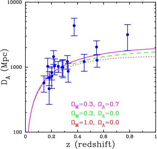
Figure 7: SZE determined distances as a function of redshift. The error bars are 68.3% statistical uncertainties only. Also plotted are the theoretical angular diameter distance relations assuming $\mbox{$H_{0}$}=60$ km s^-1 Mpc^-1 for three different cosmological models; the currently favored $\Lambda$ cosmology $\mbox{$\Omega_{M}$}=0.3$, $\mbox{$\Omega_{\Lambda}$}=0.7$ (solid) cosmology; an open $\mbox{$\Omega_{M}$}=0.3$ (dashed) universe; and a flat $\mbox{$\Omega_{M}$}=1$ (dotted) cosmology.

The column densities measured from the X-ray spectra are different from those from H I surveys (Dickey & Lockman, 1990). We use the column densities from X-ray spectral fits when possible since that includes contributions from non-neutral hydrogen and other elements which absorb X-rays. For MS0451 and Cl0016, using the survey derived column densities instead of the fitted values changes the angular diameter distance by $\sim\pm 5$% (Reese et al., 2000), which we include as a systematic uncertainty (see § 7).

Figure 7 shows the SZE determined distances for each cluster as a function of redshift. Also plotted are the theoretical angular diameter distance relations assuming $\mbox{$H_{0}$}=60$ km s^-1 Mpc^-1 for three different cosmologies: the currently favored $\Lambda$ cosmology $\mbox{$\Omega_{M}$}=0.3$, $\mbox{$\Omega_{\Lambda}$}=0.7$ (solid) cosmology; an open $\mbox{$\Omega_{M}$}=0.3$ (dashed) universe; and a flat $\mbox{$\Omega_{M}$}=1$ (dotted) cosmology. The SZE distances are beginning to probe the angular diameter distance relation. The uncertainties on $D_{\!\mbox{\tiny A}}$ in Figure 7 are the 68.3% statistical uncertainties only, including all of the statistical uncertainties in the calculation outlined above. We refer the reader to Carroll et al. (1992), Kolb & Turner (1990), and Peacock (1999) for derivations of the theoretical angular diameter distance relation.

There is a known correlation between the $\beta$ and $\theta_{c}$ parameters of the $\beta$ model. Figure 8 illustrates this correlation and its effect on $D_{\!\mbox{\tiny A}}$ for MS1358, and A2261. The filled contours are the 1, 2, and 3 $\sigma$ $\Delta S$ confidence regions for $\beta$ and $\theta_{c}$ jointly with the plus marking the best fit for each cluster. The lines are contours of constant $D_{\!\mbox{\tiny A}}$ in megaparsecs. With our interferometric SZE data, the contours of constant $D_{\!\mbox{\tiny A}}$ lie roughly parallel to the $\beta$-$\theta_{c}$ correlation, minimizing the effect of this correlation on the uncertainties of $D_{\!\mbox{\tiny A}}$. Similar figures for MS0451 and Cl0016 appear in Reese et al. (2000), which show similar behavior. The alignment of the $D_{\!\mbox{\tiny A}}$ contours with the $\beta$-$\theta_{c}$ correlation is a general feature of our observing strategy. Different observing techniques will result in different behavior. Contours of constant $D_{\!\mbox{\tiny A}}$ have been found to be roughly orthogonal to this $\beta$-$\theta_{c}$ correlation for some single dish SZE observations (Birkinshaw & Hughes, 1994; Birkinshaw et al., 1991).

To determine the Hubble Constant, we perform a $\chi^{2}$ fit to our calculated $D_{\!\mbox{\tiny A}}$’s versus $z$ for three different cosmologies. To estimate statistical uncertainties, we combine the uncertainties on $D_{\!\mbox{\tiny A}}$ listed in Table 8 in quadrature, which is only strictly valid for Gaussian distributions. This combined statistical uncertainty is symmetrized (averaged) and used in the fit. We find

$$\mbox{$H_{0}$}=\cases{60^{+4}_{-4}\ \mbox{km s${}^{-1}$ Mpc${}^{-1}$};&\mbox{$\Omega_{M}$}=0.3, \mbox{$\Omega_{\Lambda}$}=0.7,\cr 56^{+4}_{-4}\ \mbox{km s${}^{-1}$ Mpc${}^{-1}$};&\mbox{$\Omega_{M}$}=0.3, \mbox{$\Omega_{\Lambda}$}=0.0,\cr 54^{+4}_{-3}\ \mbox{km s${}^{-1}$ Mpc${}^{-1}$};&\mbox{$\Omega_{M}$}=1.0, \mbox{$\Omega_{\Lambda}$}=0.0,\cr}$$ (8)

where the uncertainties are statistical only at 68.3% confidence. The statistical error comes from the $\chi^{2}$ analysis and includes uncertainties from $T_{e}$, the parameter fitting, metallicity, $N_{\mbox{\tiny H}}$, and detected radio point sources (see Table 8). We have chosen three cosmologies encompassing the currently favored models. With this sample of clusters, there is a $\sim 10$% range in our inferred $H_{0}$ due to the geometry of the universe. For the $\Lambda$ cosmology, $\chi^{2}=16.5$ with a corresponding reduced chi-squared of $\chi^{2}_{red}=0.97$. The difference in $\chi^{2}$ between the $\mbox{$\Omega_{M}$}=0.3,\mbox{$\Omega_{\Lambda}$}=0.7$ and the flat $\mbox{$\Omega_{M}$}=1$ universes is roughly $\Delta\chi^{2}\sim 0.3$, with the $\Lambda$ cosmology having the lowest $\chi^{2}$. Clearly a larger sample of high redshift ($z\sim 1$) clusters is required for a determination of the geometry of the universe from SZE and X-ray determined direct distances to galaxy clusters (see §7).

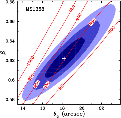
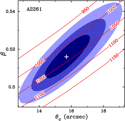
Figure 8: Confidence regions from the joint SZE and X-ray fit for MS1358 and A2261. The filled regions are 1, 2, and 3 $\sigma$ confidence regions for $\beta$ and $\theta_{c}$ jointly ($\Delta S=2.3$, 6.2, 11.8), and the cross marks the best-fit $\beta$ and $\theta_{c}$. Solid lines are contours of angular diameter distance in megaparsecs. The $D_{\!\mbox{\tiny A}}$ contours lie roughly parallel to the $\beta$-$\theta_{c}$ correlation, minimizing the effect of this correlation on the uncertainties of $D_{\!\mbox{\tiny A}}$.

6 Sources of Possible Systematic Uncertainty

Table 9: $H_{0}$ Systematic Uncertainty Budget (%)

Systematic	Effect
SZE calibration	$\pm\phantom{0}8$
X-ray calibration	$\pm 10$
$N_{\mbox{\tiny H}}$	$\pm\phantom{0}5$
Asphericity	$\pm\phantom{0}5$
Isothermality	$\pm 10$
Clumping	$-20$
Undetected radio sources	$\pm 12$
Kinetic SZE	$\pm\phantom{0}2$
Primary CMB	$<\pm 1$
Radio Halos	$-\phantom{0}3$
Primary Beam	$\pm\phantom{0}3$
Total	${}^{+22}_{-30}$

The absolute calibration of both the SZE observations and the PSPC and HRI directly affects the distance determinations. The absolute calibration of the interferometric observations is conservatively known to about 4% at 68.3% confidence, corresponding to a 8% uncertainty in $H_{0}$ ($\propto\Delta T_{0}^{-2}$). The effective areas of the PSPC and HRI are thought to be known to about 10%, introducing a 10% uncertainty into the $H_{0}$ determination through the calculation of $\Sigma$. In addition to the absolute calibration uncertainty from the observations, there are possible sources of systematic uncertainty that depend on the physical state of the ICM and other sources that can contaminate the cluster SZE emission. Table 9 summarizes the systematic uncertainties in the Hubble constant determined from our 18 cluster sample.

6.1 Cluster Atmospheres and Morphology

6.1.1 Asphericity

Most clusters do not appear circular in radio, X-rays, or optical. Fitting a projected elliptical isothermal $\beta$ model gives typical axial ratios that are close to the local average of $0.80$ (Mohr et al., 1995). Under the assumption of axisymmetric clusters, the combined effect of cluster asphericity and its orientation on the sky conspires to introduce a $\sim\pm 20$% random uncertainty in $H_{0}$ determined from one galaxy cluster (Hughes & Birkinshaw, 1998). When one considers a large, unbiased sample of clusters, with random orientations, the errors due to imposing a spherical model are expected to cancel, resulting in a precise determination of $H_{0}$. Recently, Sulkanen (1999) studied projection effects using triaxial $\beta$ models. Fitting these with spherical models he found that the Hubble constant estimated from the sample was within 5% of the input value. We are in the process of using N-body and smoothed particle hydrodynamics (SPH) simulations of 48 clusters to quantify the effects of complex cluster structure on our results.

A 20% effect from one cluster implies a 5% ($=20/\sqrt{18}$) effect for a sample of 18 clusters. Therefore, we include at 5% effect from asphericity for our cluster sample.

6.1.2 Temperature Gradients

Departures from isothermality in the cluster atmosphere may result in a large error in the distance determination from an isothermal analysis; moreover, an isothermal analysis of a large cluster sample could lead to systematic errors in the derived Hubble parameter if most clusters have similar departures from isothermality (Birkinshaw & Hughes, 1994; Inagaki et al., 1995; Holzapfel et al., 1997b). The ROSAT band is fairly insensitive to temperature variations, showing a $\sim 10$% change in the PSPC count rate for a factor of 2 change in temperature for $T_{e}>1.5$ keV gas (Mohr et al., 1999). In theory, cluster temperature profiles may significantly affect the distance determinations through the SZE since $\Delta T\propto\int n_{e}T_{e}d\ell$. The spatial filtering of the interferometer makes our SZE observations insensitive to angular scales larger than a few arcminutes. Therefore we are relatively insensitive to large scale temperature gradients. However, we are sensitive to temperature gradients on smaller scales, for example at the center of cooling flow clusters.

A mixture of simulations and studies of nearby clusters suggests a 10% effect on the Hubble parameter (Inagaki et al., 1995; Roettiger et al., 1997) due to departures from isothermality. The spatial filtering of the interferometer is not accounted for in these studies and thus provides a conservative estimate. We include a conservative $\pm 10$% effect on the inferred Hubble parameter due to departures of isothermality, consistent with both cooling flow (see §6.1.3) and non-cooling flow departures.

6.1.3 Cooling Flows

Cooling flows affect the emission weighted mean temperature and enhance the X-ray central surface brightness (see, e.g., Fabian, 1994; Nagai et al., 2000). When the cooling time at the center of the cluster is less than the age of the cluster, then the central gas has time to cool. This is known as a cooling flow (e.g., Fabian, 1994). The cluster temperature is expected to decrease towards the center of the cluster, which has recently been seen with both Chandra (e.g., Markevitch et al., 2000; Nevalainen et al., 2000) and XMM-Newton (e.g., Tamura et al., 2001).

Table 10: Ratio of $t_{cool}/t_{H}(z)$

	Cosmology ($\Omega_{M}$, $\Omega_{\Lambda}$)
Cluster	(0.3, 0.7)	(0.3, 0.0)	(1.0, 0.0)
MS1137	1.1	1.9	1.4
MS0451	1.0	1.6	1.2
Cl0016	1.5	2.5	1.9
R1347	0.1	0.2	0.1
A370	3.6	5.8	4.4
MS1358	0.4	0.7	0.5
A1995	0.9	1.5	1.2
A611	0.4	0.7	0.5
A697	1.1	1.7	1.3
A1835	0.1	0.2	0.2
A2261	0.3	0.5	0.4
A773	1.5	2.4	1.8
A2163	1.3	2.0	1.6
A520	2.1	3.3	2.6
A1689	0.3	0.5	0.4
A665	1.2	1.8	1.4
A2218	1.4	2.2	1.7
A1413	0.6	0.9	0.7

A characteristic cooling time for the ICM is the available radiative energy divided by its luminosity given by

$$t_{cool}\sim\frac{3kT_{e}n_{tot}}{2\Lambda n_{e}\mbox{$n_{\mbox{\tiny H}}$}}=\frac{3kT_{e}}{2\Lambda n_{e}}\frac{\mbox{$\mu_{\mbox{\tiny H}}$}}{\mu_{tot}},$$ (9)

where $\Lambda$ is the bolometric cooling function of the cluster and all quantities are evaluated at the center of the cluster. Cooling flows may occur if the cooling time is less than the age of the cluster, which we conservatively estimate to be the age of the universe at the redshift of observation, $t_{cool}<t_{H}(z)$.

As a check, we calculate $t_{cool}/t_{H}$ ratios for each cluster analyzed by Mohr et al. (1999). We check our cooling flow and non-cooling flow determinations versus those of Peres et al. (1998) and Fabian (1994). Of the 45 clusters in the Mohr sample, 41 have published mass deposition rates. We assume the cluster does not contain a cooling flow if its mass deposition rate is consistent with zero, otherwise it is designated as a cooling flow cluster. We are able to predict whether a cluster has a cooling flow or not with a 90% success rate, suggesting that the ratio $t_{cool}/t_{H}$ presented in equation (9) is a good predictor for the presence of a cooling flow.

The ratio $t_{cool}/t_{H}(z)$ for each cluster is summarized in Table 10 for the same three cosmologies used to determine the Hubble constant. The central densities, $n_{e0}$, used in this calculation are determined by eliminating $D_{\!\mbox{\tiny A}}$ in equations (2) and (4) in favor of $n_{e0}$. From this analysis, the seven clusters R1347, MS1358, A611, A1835, A2261, A1689, and A1413 are cooling flow clusters. Both A1995 and A1413 are borderline cases. Such clusters are expected to have falling temperatures towards the center of the cluster.

In principle, the multiphase medium expected in cooling flow clusters could introduce large biases in isothermal beta model SZE and X-ray distances (Nagai & Mohr, 2002). However, recent observations with Chandra and XMM-Newton suggest that cooling flows are not as strong as previously expected (e.g., Fabian et al., 2001; Peterson et al., 2001). To estimate the possible effects of cooling flow-like temperature profiles, we adopt the deprojected temperature profile of A1835 from an analysis of XMM-Newton observations and determine the change in the angular diameter distance introduced by this profile. The inclusion of the A1835 temperature profile reduces the angular diameter distance by $\sim 10$%, causing a $\sim 10$% underestimate in the Hubble constant from cooling flow clusters when an isothermal analysis is performed (A. D. Miller 2001, private communication). In addition, a theoretical examination of the effects of cooling flows on SZE and X-ray determined distances suggests a $\sim 10$% underestimate of $H_{0}$ from an isothermal analysis (Majumdar & Nath, 2000). Assuming all seven cooling flow clusters in our sample produce a similar 10% bias in $H_{0}$, the average underestimate in $H_{0}$ for our 18 cluster sample is $\sim 4$%.

We combine the uncertainty from cooling flow and non-cooling flow (see §6.1.2) departures from isothermality into a conservative $\pm 10$% effect on the inferred Hubble parameter.

6.1.4 Clumping; Small Scale Structure

Clumping of the intracluster gas is a potentially serious source of systematic error in the determination of the Hubble constant. Unresolved clumps in an isothermal intracluster plasma will enhance the X-ray emission by the factor

$$C\equiv\frac{\left<n_{e}^{2}\right>}{\left<n_{e}\right>^{2}}.$$ (10)

The cluster generates more X-ray emission than expected from a uniform ICM leading to an underestimate of the angular diameter distance ($\mbox{$D_{\!\mbox{\tiny A}}$}\propto S_{x}^{-1}$) and therefore an overestimate of the Hubble parameter for $C>1$. Unlike the orientation bias which averages down for a large sample of clusters, clumping must be measured in each cluster or estimated for an average cluster. Theoretical estimates of $C$ are difficult because they must account for the complicated processes that both generate and damp density enhancements, such as preheating and gas-dynamical processes.

There is currently no observational evidence of significant clumping in galaxy clusters. If clumping were significant and had large variations from cluster to cluster, we might expect larger scatter than is seen in the Hubble diagrams from SZE and X-ray distances (Figure 7; see also Birkinshaw 1999). Gas-dynamical cluster simulations provide an opportunity to test the effects of observing strategy and cluster structure on our distance determinations. These simulated clusters exhibit X-ray merger signatures consistent with those observed in real clusters and, presumably, they exhibit the appropriate complexities in their temperature structure as well. Preliminary work indicates that temperature profiles do not introduce a large error on our distances but that clumping in the ICM may bias distances low by up to $\sim 20$%. As mentioned above, there is no observational evidence of clumping within the ICM. However, merger signatures are common (Mohr et al., 1995), and the mergers are the driving mechanism behind these fluctuations in the simulated clusters (Mathiesen et al., 1999).

Clumping causes an overestimate of $H_{0}$, so we include a conservative one-sided $-20$% possible systematic due to clumping.

6.2 Possible SZE Contaminants

6.2.1 Possible Undetected Point Sources in the Field

Undetected point sources near the cluster center mask the central decrement, causing an underestimate in the magnitude of the decrement and therefore an underestimate of the angular diameter distance. The synthesized beam shapes, which include negative sidelobes, allow both underestimates and overestimates in the magnitude of the decrement. As a conservative estimate of our detection threshold, we use 3 times the rms of the high reslution map, applying a $\geq 2000\ \lambda$ cut on the baselines for each cluster data set. Placing a point source with flux equal to our detection limit near the cluster center and re-analyzing to find the change in the central decrement provides an estimate of the upper bound of the effects of undetected radio point sources.

We have additional information on the distribution of point sources in all our cluster fields from observations at lower frequencies. Sources with flux densities greater than 2 mJy at 1.4 GHz appear in the NVSS catalog (Condon et al., 1998). We use the NVSS catalog to find point sources within 400″ of each cluster center. We extrapolate the NVSS sources in our fields to 28.5 GHz using the average spectral index of radio sources in galaxy clusters $\alpha=0.77$ (Cooray et al., 1998), where $S_{\nu}\propto\nu^{-\alpha}$. Extrapolated NVSS sources with fluxes greater than our 3 $\sigma$ threshold are ruled out by the 30 GHz data and their fluxes are fixed at the maximal 30 GHz 3 $\sigma$ value. The extrapolated NVSS sources are added to to the 30 GHz visibilities data, which is re-analyzed, not accounting for the additional point sources. The uncertainty on the angular diameter distance from undetected point sources is summarized in Table 11 for each cluster field. The average over the 18 cluster fields yields a $\sim 12$% uncertainty on the Hubble parameter.

We know that clusters have central dominant (cD) galaxies, which are often radio bright. Therefore it is likely that there is a radio point source near the center of each cluster. To estimate the effects of cD galaxies on the central decrement we pick three clusters for which we do not detect a central radio point source, A697, A2261, and A1413. We add a point source fixed at the optical position of the cD (Crawford et al., 1999) and vary both the flux of the cD galaxy and the central decrement, keeping the ICM shape parameters fixed at their best-fit values. The cD fluxes are all consistent with zero and the corresponding changes in the central decrement are $\lesssim 2$%. This suggests that undetected cD galaxies do not contribute significantly to the uncertainty on the Hubble constant, $\lesssim 4$%, within our uncertainty budget for possible undetected point sources.

Table 11: Effects of Undetected Point Sources on $D_{\!\mbox{\tiny A}}$ (%)

Cluster	Effect (%)
MS1137	00
MS0451	00
CL0016	02
R1347	32
A370	06
MS1358	00
A1995	06
A611	00
A697	06
A1835	00
A2261	46
A773	06
A2163	22
A520	16
A1689	18
A665	12
A2218	00
A1413	42
Average	012

6.2.2 Kinetic SZE

Cluster peculiar velocities with respect to the CMB introduce an additional CMB spectral distortion known as the kinetic SZE. The kinetic SZE is proportional to the thermal effect but has a different spectral signature so it can be distinguished from the thermal SZE with spectral SZE observations. For a 10 keV cluster with a line-of-sight peculiar velocity of 1000 km s^-1, the kinetic SZE is $\sim 11$% of the thermal SZE at 30 GHz. Watkins (1997) presented observational evidence suggesting a one-dimensional rms peculiar velocity of $\sim 300$ km s^-1 for clusters, and recent simulations found similar results (Colberg et al., 2000). With a line-of-sight peculiar velocity of 300 km s^-1 and a more typical 8 keV cluster, the kinetic SZE is $\sim 4$% of the thermal effect, introducing up to a $\sim\pm 8$% correction to the angular diameter distance computed from one cluster. When averaged over an ensemble of clusters, the effect from peculiar velocities should cancel, manifesting itself as an additional statistical uncertainty similar to the effects of asphericity. Therefore, we include a 2% ($=8/\sqrt{18}$) effect from the kinetic SZE for our 18 cluster sample.

6.2.3 CMB Primary Anisotropies

CMB primary anisotropies have the same spectral signature as the kinetic SZE. Recent BIMA observations provide limits on primary anisotropies on the scales of the observations presented here (Dawson et al., 2001; Holzapfel et al., 2000). They place a 95% confidence upper limit to the primary CMB anisotropies of $\Delta T<19$ $\mu$K at $\ell\sim 5500$ ($\sim 2\arcmin$ scales). Thus primary CMB anisotropies are an unimportant ($\lesssim 2$%) source of uncertainty for our observations. At 68.3% confidence, primary CMB anisotropies contribute a $\lesssim 1$% uncertainty in the measured Hubble parameter. In addition, CMB primary anisotropy effects on the inferred $H_{0}$ should average out over the sample; with an 18 cluster sample CMB primary anisotropy contributes $<1$% uncertainty to $H_{0}$.

6.2.4 Radio Halos

The SZE decrement may be masked by large scale diffuse non-thermal radio emission in clusters of galaxies, known as radio halos. If present, radio halos are located at the cluster centers, have sizes typical of galaxy clusters, and a steep radio spectrum $\alpha\sim 1-3$ (Kempner & Sarazin, 2001; Giovannini et al., 1999; Moffet & Birkinshaw, 1989; Hanisch, 1982). Similar structures at the cluster periphery, usually with an irregular shape, are called relics. In general, radio halos and relics are rare phenomena that are present in rich, massive clusters, characterized by high X-ray luminosity and high temperature (Giovannini & Feretti, 2000; Giovannini et al., 1999). Cooling flow clusters rarely contain radio halos. Because halos and relics are rare, little is known about their nature and origin but they are thought to be produced by synchrotron emission from an accelerated or reaccelerated population of relativistic electrons (e.g., Jaffe, 1977; Dennison, 1980; Roland, 1981; Schlickeiser et al., 1987). Shocks from cluster mergers may be the acceleration mechanism though there are numerous theories (e.g., Jaffe, 1977, 1980; Dennison, 1980; Roland, 1981; Schlickeiser et al., 1987; Ensslin et al., 1998; Blasi & Colafrancesco, 1999; Dolag & Ensslin, 2000; Liang et al., 2000).

According to the literature (Kempner & Sarazin, 2001; Giovannini & Feretti, 2000; Giovannini et al., 1999), the following clusters in our sample exhibit radio halos: Cl0016, A773, A2163, A520, A665, A2218. In Figure 9, we show NVSS 1.4 GHz image contours (Condon et al., 1998) overlaid on color scale images of the SZE cluster emission. Contours are multiples of twice the rms in the NVSS maps (rms $\sim 0.45$ mJy beam^-1). It is apparent that many of these halos are at the 2 $\sigma\approx 0.9$ mJy beam^-1 level. The brightest known halo is seen in A2163 with a peak brightness of $\sim 5.4$ mJy beam^-1.

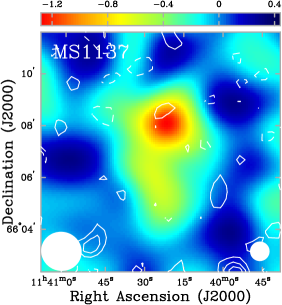
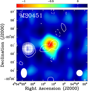
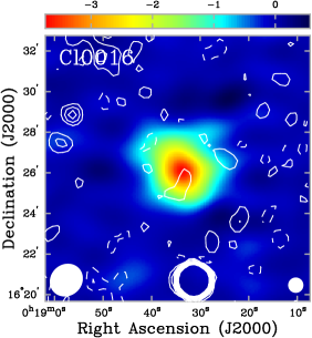
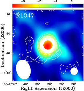
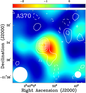
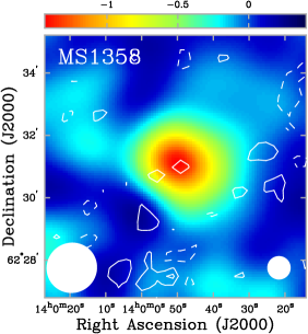
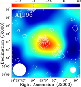
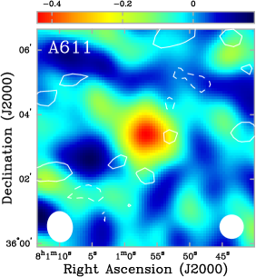
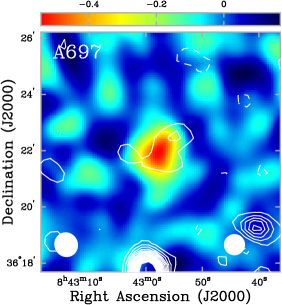
Figure 9: SZE from our own 30 GHz observations (color scale) with NVSS 1.4 GHz contours. The 30 GHz images are the color scale version of the SZE shown in Figure 2. The color scale wedge above each image shows the range in the flux density of the 30 GHz map in units of mJy beam^-1. Contours are multiples of twice the rms and the NVSS rms is $\sim 0.45$ mJy beam^-1. The FWHM of the 30 GHz synthesized beam is shown in the lower left hand corner of each panel and the 45″ FWHM beam of the NVSS survey is shown in the lower right hand corner of each panel. A2163 exhibits the brightest 1.4 GHz radio halo in our 18 cluster sample.

–Cont.

For each of the halo clusters, we conservatively model the halo as a point source at the cluster center with flux from an $\alpha=1$ extrapolation of the peak NVSS halo flux and re-analyze to determine the effect on the central decrement. The average effect on the central decrement from the clusters with radio halos in our sample is 4%, excluding A2163 which shows a $\sim 10$% effect on the central decrement. Radio halos typically have spectral indices $\alpha\geq 1.5$, making the $\alpha=1$ extrapolation a conservative upper bound for the effects of radio halos. Averaged over the entire 18 cluster sample, the $\alpha=1$ extrapolation results imply a $\sim 3$% overestimate ($-3$% effect) on our inferred Hubble parameter ($\mbox{$H_{0}$}\propto\Delta T^{-2}$) from radio halos.

6.2.5 Imprecisely Measured Primary Beam

The primary beam is determined from holography measurements at both OVRO and BIMA. The effect of the primary beam on the interferometric observations is a convolution in the Fourier plane (see §3.1.1) or equivalently, an attenuation across the field of view. Therefore, differences in primary beam shape simply alter the smoothing kernel in the $u$-$v$ plane only slightly, having a small affect on the derived distances.

To assess the effects of the primary beam quantitatively, we fit to an OVRO and BIMA data set using a cluster model attenuated by a Gaussian beam with different assumed FWHMs. There is no significant change in the central decrements when using a Gaussian approximation for the primary beam instead of the measured beam. Even with an unrealistically large $\pm 0.2\arcmin$ uncertainty in the primary beam FWHM, the uncertainty introduced in the Hubble constant is $\lesssim 3$% ($\lesssim 2$% in $\Delta T_{0}$). Artificially broadening the wings of the real beam has a negligible effect on the derived central decrements. We adopt a 3% uncertainty in $H_{0}$ as a conservative estimate of the maximum effects from an imprecisely measured primary beam.

7 Discussion and Conclusion

We perform a maximum-likelihood joint fit to centimeter-wave interferometric SZE and ROSAT X-ray (PSPC and HRI) data to constrain the ICM parameters for a sample of high redshift clusters of galaxies. We model the ICM as a spherical, isothermal $\beta$ model. From this analysis we determine the distances to 18 galaxy clusters. Together, these distances imply a Hubble constant of

$$\mbox{$H_{0}$}=\cases{60^{+4}_{-4}\,{}^{+13}_{-18}\ \mbox{km s${}^{-1}$ Mpc${}^{-1}$};&\mbox{$\Omega_{M}$}=0.3, \mbox{$\Omega_{\Lambda}$}=0.7,\cr 56^{+4}_{-4}\,{}^{+12}_{-17}\ \mbox{km s${}^{-1}$ Mpc${}^{-1}$};&\mbox{$\Omega_{M}$}=0.3, \mbox{$\Omega_{\Lambda}$}=0.0,\cr 54^{+4}_{-3}\,{}^{+12}_{-16}\ \mbox{km s${}^{-1}$ Mpc${}^{-1}$};&\mbox{$\Omega_{M}$}=1.0, \mbox{$\Omega_{\Lambda}$}=0.0,\cr}$$ (11)

where the uncertainties are statistical followed by systematic at 68.3% confidence. The systematic uncertainties have been added in quadrature and include an 8% (4% in $\Delta T_{0}$) uncertainty from the absolute calibration of the SZE data, a 10% effective area uncertainty for the PSPC and HRI, a 5% uncertainty from the column density, a 5% ($\simeq 20/\sqrt{18}$) uncertainty due to asphericity, a 10% effect for our assumptions of isothermality, a one-sided $-20$% effect from possible small-scale clumping in the ICM, a 12% uncertainty from undetected radio sources, a 2% ($\simeq 8/\sqrt{18}$) uncertainty from the kinetic SZE, a 1% uncertainty from primary CMB anisotropies, a $-3$% effect from radio halos, and a 3% effect from an imprecisely measured primary beam. These systematic uncertainties are summarized in Table 9. We adopt conservative assumptions when gauging the effects of possible systematics. The contributions from asphericity, kinetic SZE, and primary CMB are expected to average out for a large sample.

The measured distances plotted in Figure 7 with the theoretical relation show that A370 is the largest outlier from the theoretical angular diameter distance relation and MS1137 has the largest distance uncertainty. A370 exhibits an almost 2-to-1 axial ratio in the knotty N-S elongation of its X-ray image (see Fig 2). An optical study of this cluster and its member galaxies shows that the cluster is dominated by two giant elliptical galaxies with a projected separation of about 40″, roughly in the north-south direction (Mellier et al., 1988). In addition, gravitational lens models suggest that A370 has a bimodal mass distribution with the two components separated in a roughly north-south direction (Kneib et al., 1993; Soucail et al., 1988; Smail et al., 1996). The spherical model used is clearly insufficient for the complex structure of this cluster. The uncertainties on the distance to MS1137 are particularly large since MS1137 resides in the distant universe ($z=0.78$), making it difficult to collect large numbers of X-ray photons. Therefore, the uncertainties on the X-ray driven quantities are large; in particular, the uncertainty on the measured X-ray temperature is the main contributor to the large uncertainty on the angular diameter distance to MS1137. The large uncertainties on the distances to both A370 and MS1137 mean that those clusters contribute little weight in the determination of the Hubble constant.

As discussed in §2, target clusters were originally chosen from a limited sample of known X-ray clusters. We construct subsamples of our cluster sample to explore the robustness of our result and to look for possible biases in our $H_{0}$ determination. A description of the subsamples, the number of clusters in each subsample $N$, the Hubble constant from each subsample, and the $\chi^{2}$ and reduced $\chi^{2}$ for the Hubble parameter are summarized in Table 12 for each subsample considered. Only the $\mbox{$\Omega_{M}$}=0.3$, $\mbox{$\Omega_{\Lambda}$}=0.7$ cosmology is considered in this study. Other cosmologies will have similar changes to the best fit Hubble parameter. Table 12 shows that excluding the largest outlier, A370, has a negligible effect on the determined Hubble parameter. We also split the sample up based on having a cooling flow, by redshift, presence of a radio halo, based on point sources, based on right ascension and declination, based on X-ray luminosity, and based on membership in the EMSS survey or being an Abell cluster.

Table 12: $H_{0}$ from Different Subsamples for the $\Lambda$ Cosmology

		$H_{0}$
Subsample	$N$	(km s-1 Mpc-1)	$\chi^{2}$	$\chi^{2}_{red}$
All	18	$60^{+4\phantom{0}}_{-4\phantom{0}}$	16.5	0.97
No A370	17	$61^{+4\phantom{0}}_{-4\phantom{0}}$	10.8	0.68
No MS1137 or A370	16	$61^{+5\phantom{0}}_{-4\phantom{0}}$	09.8	0.65
No cooling flow	11	$59^{+6\phantom{0}}_{-5\phantom{0}}$	14.5	1.45
Only cooling flow	07	$63^{+7\phantom{0}}_{-6\phantom{0}}$	01.7	0.28
$z>0.27$	09	$62^{+7\phantom{0}}_{-6\phantom{0}}$	09.7	1.21
$z<0.27$	09	$59^{+6\phantom{0}}_{-5\phantom{0}}$	06.6	0.83
No point sources	04	$53^{+9\phantom{0}}_{-7\phantom{0}}$	03.4	1.13
Only point sources	14	$62^{+5\phantom{0}}_{-4\phantom{0}}$	12.2	0.94
Only radio halo	06	$56^{+8\phantom{0}}_{-6\phantom{0}}$	06.7	1.34
No halo	12	$62^{+5\phantom{0}}_{-5\phantom{0}}$	09.3	0.85
RA$<11.5^{\mbox{h}}$	09	$61^{+7\phantom{0}}_{-6\phantom{0}}$	13.6	1.70
RA$>11.5^{\mbox{h}}$	09	$60^{+6\phantom{0}}_{-5\phantom{0}}$	02.9	0.36
Dec$>30^{\circ}$	09	$60^{+7\phantom{0}}_{-6\phantom{0}}$	08.3	1.04
Dec$<30^{\circ}$	09	$61^{+6\phantom{0}}_{-5\phantom{0}}$	08.1	1.01
$\mbox{$L_{\!\mbox{\tiny X}}$}>14.5\times 10^{44}$ erg s-1	09	$63^{+6\phantom{0}}_{-5\phantom{0}}$	04.4	0.55
$\mbox{$L_{\!\mbox{\tiny X}}$}\leq 14.5\times 10^{44}$ erg s-1	09	$57^{+7\phantom{0}}_{-5\phantom{0}}$	11.5	1.44
EMSS clusters	05	$66^{+10}_{-8\phantom{0}}$	03.5	0.88
Abell clusters	13	$58^{+5\phantom{0}}_{-4\phantom{0}}$	12.2	1.02
Orientation unbiased	06	$58^{+8\phantom{0}}_{-6\phantom{0}}$	6.2	1.24

Jones et al. (2002) constructed an orientation unbiased sample of galaxy clusters for a SZE and X-ray determination of the Hubble parameter. Most importantly, they drew clusters present in both the BCS (Ebeling et al., 2000a; Crawford et al., 1999; Ebeling et al., 1998, 1997) and NORAS (Böhringer et al., 2000) surveys with $\mbox{$L_{\!\mbox{\tiny X}}$}>8\times 10^{44}$ erg s^-1 and well above the survey flux limits ($>5\times 10^{-12}$ erg s^-1 cm^-2). Eleven clusters satisfy these criterion as well as their redshift range choice ($0.14\leq z\leq 0.30$) and declination constraint ($\geq 2^{\circ}$). They find five of the eleven to be sufficiently free from point sources at 15 GHz for SZE measurements. Six of these eleven are part of our sample, which we call our orientation unbiased subsample in Table 12.

All of these subsamples yield a Hubble constant with 1 $\sigma$ statistical uncertainties consistent with the $H_{0}$ from the entire 18 cluster sample. This argues in favor of a robust $H_{0}$ determination.

We compare our results with other SZE determined distances to clusters in our sample in Table 13. Only statistical uncertainties are included. There are nine clusters in our sample that also have previously determined SZE distances. All of the 1 $\sigma$ confidence regions agree with our own, with the exception of Cl0016, R1347, A773, and A665. The systematic uncertainties on the angular diameter distance are $\gtrsim 30$% for one galaxy cluster. Therefore, all of the distances are in reasonably good agreement, even after accounting for shared systematics (namely most use ROSAT X-ray data and ASCA X-ray temperatures).

Table 13: Comparison of SZE Determined Distances

	$D_{\!\mbox{\tiny A}}$
Cluster	(Mpc)	reference
Cl0016	$2041\pm 499$	This work
	$1788\pm 664$	H98
	$1100\pm 295$	G02
R1347	$1221\pm 356$	This work
	$1890\pm 644$	P01
	$1897\pm 401$	K99
A697	$\phantom{0}998\pm 274$	This work
	$1044\pm 239$	J02
A1835	$1027\pm 196$	This work
	$\phantom{0}867\pm 411$	M00
A773	$1450\pm 347$	This work
	$1002\pm 257$	S99
A2163	$\phantom{0}828\pm 193$	This work
	$\phantom{0}728\pm 387$	H97
	$\phantom{0}615\pm 327$	L98
A665	$\phantom{0}466\pm 198$	This work
	$1017\pm 229$	B91
A2218	$1029\pm 346$	This work
	$\phantom{0}616\pm 118$	B94
	$\phantom{0}720\pm 422$	T98
	$1201\pm 343$	J02
A1413	$\phantom{0}573\pm 161$	This work
	$\phantom{0}565\pm 164$	G02b

Many of the systematics can be approached and reduced through improved observations. For example, Chandra and XMM-Newton are now producing temperature profiles of galaxy clusters (e.g., Markevitch et al., 2000; Nevalainen et al., 2000; Tamura et al., 2001). The unprecedented angular resolution of Chandra will provide insight into possible clumping in clusters. The effects of undetected point sources are being addressed with multi-wavelength (5 and 8 GHz) VLA observations of many of our cluster fields. In addition, there is a project to produce a $\sim 1$% calibration of the modified OVRO and BIMA SZE systems and the current generation of X-ray satellites will reduce the X-ray absolute calibration uncertainty to the few percent level.

The 18 cluster distances presented here are beginning to probe the shape of the angular diameter distance relation. Moreover, constructing subsamples from our 18 cluster sample based on such considerations as cooling flows, redshift, and X-ray luminosity, does not significantly affect the best fit $H_{0}$, suggesting a robust determination of the Hubble parameter. Systematics currently dominate the uncertainty in our determination of the Hubble parameter. These systematics can and will be addressed with current radio observatories (OVRO, BIMA, and VLA) and X-ray satellites (Chandra and XMM-Newton). With a sample of high redshift galaxy clusters, this method can be used to constrain the geometry of the universe, providing a valuable independent check of the recent supernovae type Ia (Schmidt et al., 1998; Riess et al., 1998; Perlmutter et al., 1999; Goobar et al., 2000) and primary CMB power spectrum results (Pryke et al., 2002; de Bernardis et al., 2002; Stompor et al., 2001). We emphasize that SZE and X-ray determined distances are independent of the extragalactic distance latter and do not rely on clusters being standard candles or rulers.

A complete review of other distance determination methods is beyond the scope of this paper. We will just touch on a few methods that complement SZE determined distances. The SZE derived distances are direct, making them an interesting check of the cosmological distance ladder. Our measurement of $H_{0}$ in the distant universe, agrees within the uncertainties with the Hubble Space Telescope (HST) $H_{0}$ Key Project results, which probes the nearby universe. The HST $H_{0}$ Key Project finds $\mbox{$H_{0}$}=72\pm 3\pm 7$ km s^-1 Mpc^-1 (Freedman et al., 2001), where the uncertainties are statistical followed by systematic at 68.3% confidence. Though few in number, there are other methods that yield distances that are independent of the extragalactic distance ladder. Recent observations of masers orbiting the nucleus of the nearby galaxy NGC 4258 (Herrnstein et al., 1999) illustrate a method of determining direct distances in the nearby universe. Time delays produced by lensing of QSO’s by galaxies are another direct distance indicator that can probe the high-redshift universe (for recent examples, see Fassnacht et al., 1999; Biggs et al., 1999; Lovell et al., 1998; Barkana, 1997; Schechter et al., 1997).

SZE surveys provide a promising method of detecting high redshift galaxy clusters (e.g., Holder et al., 2000; Barbosa et al., 1996). These surveys will provide large catalogs of high redshift galaxy clusters required to determine the geometry of the universe from SZE and X-ray determined direct distances.

References

- Allen (2000) Allen, S. W. 2000, MNRAS, 315, 269
- Allen & Fabian (1998a) Allen, S. W. & Fabian, A. C. 1998a, MNRAS, 297, L57
- Allen & Fabian (1998b) —. 1998b, MNRAS, 297, L63
- Arnaud & Evrard (1999) Arnaud, M. & Evrard, A. E. 1999, MNRAS, 305, 631
- Barbosa et al. (1996) Barbosa, D., Bartlett, J. G., Blanchard, A., & Oukbir, J. 1996, A&A, 314, 13
- Barkana (1997) Barkana, R. 1997, ApJ, 489, 21
- Biggs et al. (1999) Biggs, A. D., Browne, I. W. A., Helbig, P., Koopmans, L. V. E., Wilkinson, P. N., & Perley, R. A. 1999, MNRAS, 304, 349
- Birkinshaw (1999) Birkinshaw, M. 1999, Physics Reports, 310, 97
- Birkinshaw & Hughes (1994) Birkinshaw, M. & Hughes, J. P. 1994, ApJ, 420, 33
- Birkinshaw et al. (1991) Birkinshaw, M., Hughes, J. P., & Arnaud, K. A. 1991, ApJ, 379, 466
- Blasi & Colafrancesco (1999) Blasi, P. & Colafrancesco, S. 1999, Astroparticle Physics, 12, 169
- Böhringer et al. (2000) Böhringer, H., et al. 2000, ApJS, 129, 435
- Cannon et al. (1999) Cannon, D. B., Ponman, T. J., & Hobbs, I. S. 1999, MNRAS, 302, 9
- Carlstrom et al. (1998) Carlstrom, J. E., Grego, L., Holzapfel, W. L., & Joy, M. 1998, Eighteenth Texas Symposium on Relativistic Astrophysics and Cosmology, ed A. Olinto, J. Frieman, and D. Schramm, World Scientific, 261
- Carlstrom et al. (1996) Carlstrom, J. E., Joy, M., & Grego, L. 1996, ApJ, 456, L75
- Carlstrom et al. (2000) Carlstrom, J. E., Joy, M., Grego, L., Holder, G., Holzapfel, W. L., LaRoque, S., Mohr, J. J., & Reese, E. D. 2000, in Constructing the Universe with Clusters of Galaxies, ed. F. Durret & G. Gerbal, IAP
- Carroll et al. (1992) Carroll, S. M., Press, W. H., & Turner, E. L. 1992, ARA&A, 30, 499
- Cash (1979) Cash, W. 1979, ApJ, 228, 939
- Cavaliere & Fusco-Femiano (1976) Cavaliere, A. & Fusco-Femiano, R. 1976, A&A, 49, 137
- Cavaliere & Fusco-Femiano (1978) —. 1978, A&A, 70, 677
- Challinor & Lasenby (1998) Challinor, A. & Lasenby, A. 1998, ApJ, 499, 1
- Colberg et al. (2000) Colberg, J. M., White, S. D. M., MacFarland, T. J., Jenkins, A., Pearce, F. R., Frenk, C. S., Thomas, P. A., & Couchman, H. M. P. 2000, MNRAS, 313, 229
- Condon et al. (1998) Condon, J. J., Cotton, W. D., Greisen, E. W., Yin, Q. F., Perley, R. A., Taylor, G. B., & Broderick, J. J. 1998, AJ, 115, 1693
- Conroy et al. (1993) Conroy, M. A., Deponte, J., Moran, J. F., Orszak, J. S., Roberts, W. P., & Schmidt, D. 1993, in ASP Conf. Ser. 52: Astronomical Data Analysis Software and Systems II, ed. . J. B. R. J. Hanisch, R. J. V. Brissenden, Vol. 2, 238
- Cooray et al. (1998) Cooray, A. R., Grego, L., Holzapfel, W. L., Joy, M., & Carlstrom, J. E. 1998, AJ, 115, 1388
- Crawford et al. (1999) Crawford, C. S., Allen, S. W., Ebeling, H., Edge, A. C., & Fabian, A. C. 1999, MNRAS, 306, 857
- Crawford et al. (1995) Crawford, C. S., Edge, A. C., Fabian, A. C., Allen, S. W., Bohringer, H., Ebeling, H., McMahon, R. G., & Voges, W. 1995, MNRAS, 274, 75
- Dawson et al. (2001) Dawson, K. S., Holzapfel, W. L., Carlstrom, J. E., Joy, M., LaRoque, S. J., & Reese, E. D. 2001, ApJ, 553, L1
- de Bernardis et al. (2002) de Bernardis, P., et al. 2002, ApJ, 564, 559
- Dell’Antonio et al. (1995) Dell’Antonio, I. P., Geller, M. J., & Fabricant, D. G. 1995, AJ, 110, 502
- Dennison (1980) Dennison, B. 1980, ApJ, 239, L93
- Dickey & Lockman (1990) Dickey, J. M. & Lockman, F. J. 1990, ARA&A, 28, 215
- Dolag & Ensslin (2000) Dolag, K. & Ensslin, T. A. 2000, A&A, 362, 151
- Dolgov et al. (2001) Dolgov, A. D., Hansen, S. H., Pastor, S., & Semikoz, D. V. 2001, ApJ, 554, 74
- Donahue (1996) Donahue, M. 1996, ApJ, 468, 79
- Donahue et al. (1999) Donahue, M., Voit, G. M., Scharf, C. A., Gioia, I. M., Mullis, C. R., Hughes, J. P., & Stocke, J. T. 1999, ApJ, 527, 525
- Dressler & Gunn (1992) Dressler, A. & Gunn, J. E. 1992, ApJS, 78, 1
- Ebeling et al. (2000a) Ebeling, H., Edge, A. C., Allen, S. W., Crawford, C. S., Fabian, A. C., & Huchra, J. P. 2000a, MNRAS, 318, 333
- Ebeling et al. (1998) Ebeling, H., Edge, A. C., Bohringer, H., Allen, S. W., Crawford, C. S., Fabian, A. C., Voges, W., & Huchra, J. P. 1998, MNRAS, 301, 881
- Ebeling et al. (1997) Ebeling, H., Edge, A. C., Fabian, A. C., Allen, S. W., Crawford, C. S., & Boehringer, H. 1997, ApJ, 479, L101
- Ebeling et al. (2001) Ebeling, H., Edge, A. C., & Henry, J. P. 2001, ApJ, 553, 668
- Ebeling et al. (2000b) Ebeling, H., et al. 2000b, ApJ, 534, 133
- Ebeling et al. (1996a) Ebeling, H., Voges, W., Bohringer, H., Edge, A. C., Huchra, J. P., & Briel, U. G. 1996a, MNRAS, 283, 1103
- Ebeling et al. (1996b) —. 1996b, MNRAS, 281, 799
- Elbaz et al. (1995) Elbaz, D., Arnaud, M., & Böhringer, H. 1995, A&A, 293, 337
- Ensslin et al. (1998) Ensslin, T. A., Biermann, P. L., Klein, U., & Kohle, S. 1998, A&A, 332, 395
- Fabian (1994) Fabian, A. C. 1994, ARA&A, 32, 277
- Fabian et al. (2001) Fabian, A. C., Mushotzky, R. F., Nulsen, P. E. J., & Peterson, J. R. 2001, MNRAS, 321, L20
- Fairley et al. (2000) Fairley, B. W., Jones, L. R., Scharf, C., Ebeling, H., Perlman, E., Horner, D., Wegner, G., & Malkan, M. 2000, MNRAS, 315, 669
- Fassnacht et al. (1999) Fassnacht, C. D., Pearson, T. J., Readhead, A. C. S., Browne, I. W. A., Koopmans, L. V. E., Myers, S. T., & Wilkinson, P. N. 1999, ApJ, 527, 498
- Fixsen et al. (1996) Fixsen, D. J., Cheng, E. S., Gales, J. M., Mather, J. C., Shafer, R. A., & Wright, E. L. 1996, ApJ, 473, 576
- Freedman et al. (2001) Freedman, W. L., et al. 2001, ApJ, 553, 47
- Geller & Beers (1982) Geller, M. J. & Beers, T. C. 1982, PASP, 94, 421
- Gioia & Luppino (1994) Gioia, I. M. & Luppino, G. A. 1994, ApJS, 94, 583
- Gioia et al. (1990) Gioia, I. M., Maccacaro, T., Schild, R. E., Wolter, A., Stocke, J. T., Morris, S. L., & Henry, J. P. 1990, ApJS, 72, 567
- Giovannini & Feretti (2000) Giovannini, G. & Feretti, L. 2000, New Astronomy, 5, 335
- Giovannini et al. (1999) Giovannini, G., Tordi, M., & Feretti, L. 1999, New Astronomy, 4, 141
- Girardi et al. (1997) Girardi, M., Fadda, D., Escalera, E., Giuricin, G., Mardirossian, F., & Mezzetti, M. 1997, ApJ, 490, 56
- Gómez et al. (2000) Gómez, P. L., Hughes, J. P., & Birkinshaw, M. 2000, ApJ, 540, 726
- Goobar et al. (2000) Goobar, A., et al. 2000, Physica Scripta Volume T, 85, 47
- Gould (1980) Gould, R. J. 1980, ApJ, 238, 1026
- Grainge et al. (2002a) Grainge, K., Grainger, W. F., Jones, M. E., Kneissl, R., Pooley, G. G., & Saunders, R. 2002a, MNRAS, 329, 890
- Grainge et al. (1993) Grainge, K., Jones, M., Pooley, G., Saunders, R., & Edge, A. 1993, MNRAS, 265, L57
- Grainge et al. (2002b) Grainge, K., Jones, M. E., Pooley, G., Saunders, R., Edge, A., & Kneissl, R. 2002b, MNRAS–submitted: astro-ph/9904165
- Grego et al. (2000) Grego, L., Carlstrom, J. E., Joy, M. K., Reese, E. D., Holder, G. P., Patel, S., Cooray, A. R., & Holzapfel, W. L. 2000, ApJ, 539, 39
- Grego et al. (2001) Grego, L., Carlstrom, J. E., Reese, E. D., Holder, G. P., Holzapfel, W. L., Joy, M. K., Mohr, J. J., & Patel, S. 2001, ApJ, 552, 2
- Hanisch (1982) Hanisch, R. J. 1982, A&A, 116, 137
- Herbig et al. (1995) Herbig, T., Lawrence, C. R., Readhead, A. C. S., & Gulkis, S. 1995, ApJ, 449, L5
- Herrnstein et al. (1999) Herrnstein, J. R., et al. 1999, Nature, 400, 539
- Holder et al. (2000) Holder, G. P., Mohr, J. J., Carlstrom, J. E., Evrard, A. E., & Leitch, E. M. 2000, ApJ, 544, 629
- Holzapfel et al. (1997a) Holzapfel, W. L., et al. Ade, P. A. R., Church, S. E., Mauskopf, P. D., Rephaeli, Y., Wilbanks, T. M., & Lange, A. E. 1997a, ApJ, 481, 35
- Holzapfel et al. (1997b) Holzapfel, W. L., et al. 1997b, ApJ, 480, 449
- Holzapfel et al. (2000) Holzapfel, W. L., Carlstrom, J. E., Grego, L., Holder, G., Joy, M., & Reese, E. D. 2000, ApJ, 539, 57
- Hughes & Birkinshaw (1998) Hughes, J. P. & Birkinshaw, M. 1998, ApJ, 501, 1
- Inagaki et al. (1995) Inagaki, Y., Suginohara, T., & Suto, Y. 1995, PASJ, 47, 411
- Itoh et al. (1998) Itoh, N., Kohyama, Y., & Nozawa, S. 1998, ApJ, 502, 7
- Jaffe (1980) Jaffe, W. 1980, ApJ, 241, 925
- Jaffe (1977) Jaffe, W. J. 1977, ApJ, 212, 1
- Jones et al. (1998) Jones, L. R., Scharf, C., Ebeling, H., Perlman, E., Wegner, G., Malkan, M., & Horner, D. 1998, ApJ, 495, 100
- Jones et al. (1993) Jones, M., et al. 1993, Nature, 365, 320
- Jones et al. (2002) Jones, M. E., et al. 2002, MNRAS– submitted: astro-ph/0103046
- Kalloglyan et al. (1990) Kalloglyan, A. T., Nanni, D., & Vignato, A. 1990, Astrophysics, 31, 672
- Kempner & Sarazin (2001) Kempner, J. C. & Sarazin, C. L. 2001, ApJ, 548, 639
- Kendall & Stuart (1979) Kendall, M. & Stuart, A. 1979, The Advanced Theory of Statistics. Vol.2: Inference and Relationship (London: Griffin, 1979, 4th ed.), 246
- Kneib et al. (1993) Kneib, J. P., Mellier, Y., Fort, B., & Mathez, G. 1993, A&A, 273, 367
- Kneib et al. (1995) Kneib, J. P., Mellier, Y., Pello, R., Miralda-Escude, J., Le Borgne, J. ., Boehringer, H., & Picat, J. . 1995, A&A, 303, 27
- Kolb & Turner (1990) Kolb, E. W. & Turner, M. S. 1990, in Frontiers in Physics, Reading, MA: Addison-Wesley, 1988, 1990
- Komatsu et al. (1999) Komatsu, E., Kitayama, T., Suto, Y., Hattori, M., Kawabe, R., Matsuo, H., Schindler, S., & Yoshikawa, K. 1999, ApJ, 516, L1
- Lamarre et al. (1998) Lamarre, J. M., et al. 1998, ApJ, 507, L5
- Le Borgne et al. (1992) Le Borgne, J. F., Pello, R., & Sanahuja, B. 1992, A&AS, 95, 87
- Liang et al. (2000) Liang, H., Hunstead, R. W., Birkinshaw, M., & Andreani, P. 2000, ApJ, 544, 686
- Lovell et al. (1998) Lovell, J. E. J., Jauncey, D. L., Reynolds, J. E., Wieringa, M. H., King, E. A., Tzioumis, A. K., McCulloch, P. M., & Edwards, P. G. 1998, ApJ, 508, L51
- Maccacaro et al. (1994) Maccacaro, T., Wolter, A., McLean, B., Gioia, I. M., Stocke, J. T., della Ceca, R., Burg, R., & Faccini, R. 1994, Astrophys. Lett., 29, 267
- Majumdar & Nath (2000) Majumdar, S. & Nath, B. B. 2000, ApJ, 542, 597
- Markevitch (1997) Markevitch, M. 1997, ApJ, 483, L17
- Markevitch et al. (1996) Markevitch, M., Mushotzky, R., Inoue, H., Yamashita, K., Furuzawa, A., & Tawara, Y. 1996, ApJ, 456, 437
- Markevitch et al. (2000) Markevitch, M., et al. 2000, ApJ, 541, 542
- Mason (1999) Mason, B. S. 1999, PhD thesis, University of Pennsylvania
- Mason et al. (2001) Mason, B. S., Myers, S. T., & Readhead, A. C. S. 2001, ApJ, 555, L11
- Mathiesen et al. (1999) Mathiesen, B., Evrard, A. E., & Mohr, J. J. 1999, ApJ, 520, L21
- Mauskopf et al. (2000) Mauskopf, P. D., et al. 2000, ApJ, 538, 505
- Mellier et al. (1988) Mellier, Y., Soucail, G., Fort, B., & Mathez, G. 1988, A&A, 199, 13
- Moffet & Birkinshaw (1989) Moffet, A. T. & Birkinshaw, M. 1989, AJ, 98, 1148
- Mohr et al. (1995) Mohr, J. J., Evrard, A. E., Fabricant, D. G., & Geller, M. J. 1995, ApJ, 447, 8
- Mohr et al. (1999) Mohr, J. J., Mathiesen, B., & Evrard, A. E. 1999, ApJ, 517, 627
- Molnar & Birkinshaw (1999) Molnar, S. M. & Birkinshaw, M. 1999, ApJ, 523, 78
- Mushotzky & Scharf (1997) Mushotzky, R. F. & Scharf, C. A. 1997, ApJ, 482, L13
- Myers et al. (1997) Myers, S. T., Baker, J. E., Readhead, A. C. S., Leitch, E. M., & Herbig, T. 1997, ApJ, 485, 1
- Nagai & Mohr (2002) Nagai, D. & Mohr, J. J. 2002, ApJ– submitted
- Nagai et al. (2000) Nagai, D., Sulkanen, M. E., & Evrard, A. E. 2000, MNRAS, 316, 120
- Nevalainen et al. (2000) Nevalainen, J., Markevitch, M., & Forman, W. 2000, ApJ, 536, 73
- Ota et al. (1998) Ota, N., Mitsuda, K., & Fukazawa, Y. 1998, ApJ, 495, 170
- Patel et al. (2000) Patel, S. K., et al. 2000, ApJ, 541, 37
- Peacock (1999) Peacock, J. A. 1999, Cosmological physics (Cosmological physics. Publisher: Cambridge, UK: Cambridge University Press, 1999. ISBN: 0521422701)
- Pearson et al. (1994) Pearson, T. J., Shepherd, M. C., Taylor, G. B., & Myers, S. T. 1994, BAAS, 185, 0808
- Peres et al. (1998) Peres, C. B., Fabian, A. C., Edge, A. C., Allen, S. W., Johnstone, R. M., & White, D. A. 1998, MNRAS, 298, 416
- Perlmutter et al. (1999) Perlmutter, S., et al. 1999, ApJ, 517, 565
- Peterson et al. (2001) Peterson, J. R., et al. 2001, A&A, 365, L104
- Pointecouteau et al. (2001) Pointecouteau, E., Giard, M., Benoit, A., Désert, F. X., Bernard, J. P., Coron, N., & Lamarre, J. M. 2001, ApJ, 552, 42
- Pointecouteau et al. (1999) Pointecouteau, E., Giard, M., Benoit, A., Désert, F. X., Aghanim, N., Coron, N., Lamarre, J. M., & Delabrouille, J. 1999, ApJ, 519, L115
- Pospieszalski et al. (1995) Pospieszalski, M. W., Lakatosh, W. J., Nguyen, L. D., Lui, M., Liu, T., Le, M., Thompson, M. A., & Delaney, M. J. 1995, IEEE MTT-S Int. Microwave Symp., 1121
- Pryke et al. (2002) Pryke, C., Halverson, N. W., Leitch, E. M., Kovac, J., Carlstrom, J. E., Holzapfel, W. L., & Dragovan, M. 2002, ApJ, 568, 46
- Raymond & Smith (1977) Raymond, J. C. & Smith, B. W. 1977, ApJS, 35, 419
- Reese et al. (2000) Reese, E. D., et al. 2000, ApJ, 533, 38
- Rephaeli (1995) Rephaeli, Y. 1995, ApJ, 445, 33
- Rephaeli & Yankovitch (1997) Rephaeli, Y. & Yankovitch, D. 1997, ApJ, 481, L55
- Riess et al. (1998) Riess, A. G., et al. 1998, AJ, 116, 1009
- Roettiger et al. (1997) Roettiger, K., Stone, J. M., & Mushotzky, R. F. 1997, ApJ, 482, 588
- Roland (1981) Roland, J. 1981, A&A, 93, 407
- Rudy (1987) Rudy, D. J. 1987, PhD thesis, California Inst. of Tech., Pasadena.
- Sault et al. (1995) Sault, R. J., Teuben, P. J., & Wright, M. C. H. 1995, ASP Conf. Ser. 77: Astronomical Data Analysis Software and Systems IV, 4, 433
- Saunders et al. (1999) Saunders, R., et al. 1999, MNRAS–submitted: astro-ph/9904168
- Sazonov & Sunyaev (1998a) Sazonov, S. Y. & Sunyaev, R. A. 1998a, ApJ, 508, 1
- Sazonov & Sunyaev (1998b) —. 1998b, Astronomy Letters, 24, 553
- Scharf et al. (1997) Scharf, C. A., Jones, L. R., Ebeling, H., Perlman, E., Malkan, M., & Wegner, G. 1997, ApJ, 477, 79
- Schechter et al. (1997) Schechter, P. L., et al. 1997, ApJ, 475, L85
- Schindler et al. (1995) Schindler, S., et al. 1995, A&A, 299, L9
- Schindler et al. (1997) Schindler, S., Hattori, M., Neumann, D. M., & Boehringer, H. 1997, A&A, 317, 646
- Schlickeiser et al. (1987) Schlickeiser, R., Sievers, A., & Thiemann, H. 1987, A&A, 182, 21
- Schmidt et al. (1998) Schmidt, B. P., et al. 1998, ApJ, 507, 46
- Scoville et al. (1993) Scoville, N. Z., Carlstrom, J. E., Chandler, C. J., Phillips, J. A., Scott, S. L., Tilanus, R. P. J., & Wang, Z. 1993, PASP, 105, 1482
- Smail et al. (1996) Smail, I., Dressler, A., Kneib, J., Ellis, R. S., Couch, W. J., Sharples, R. M., & Oemler, A. J. 1996, ApJ, 469, 508
- Snowden (1998) Snowden, S. L. 1998, ApJS, 117, 233
- Snowden et al. (1994) Snowden, S. L., McCammon, D., Burrows, D. N., & Mendenhall, J. A. 1994, ApJ, 424, 714
- Soucail et al. (1988) Soucail, G., Mellier, Y., Fort, B., Mathez, G., & Cailloux, M. 1988, A&A, 191, L19
- Stebbins (1997) Stebbins, A. 1997, preprint: astro-ph/9709065
- Stocke et al. (1991) Stocke, J. T., Morris, S. L., Gioia, I. M., Maccacaro, T., Schild, R., Wolter, A., Fleming, T. A., & Henry, J. P. 1991, ApJS, 76, 813
- Stompor et al. (2001) Stompor, R., et al. 2001, ApJ, 561, L7
- Struble & Rood (1991) Struble, M. F. & Rood, H. J. 1991, ApJS, 77, 363
- Struble & Rood (1999) —. 1999, ApJS, 125, 35
- Sulkanen (1999) Sulkanen, M. E. 1999, ApJ, 522, 59
- Sunyaev & Zel’dovich (1970) Sunyaev, R. A. & Zel’dovich, Y. B. 1970, Comments Astrophys. Space Phys., 2, 66
- Sunyaev & Zel’dovich (1972) —. 1972, Comments Astrophys. Space Phys., 4, 173
- Tamura et al. (2001) Tamura, T., et al. 2001, A&A, 365, L87
- Tsuboi et al. (1998) Tsuboi, M., Miyazaki, A., Kasuga, T., Matsuo, H., & Kuno, N. 1998, PASJ, 50, 169
- Watkins (1997) Watkins, R. 1997, MNRAS, 292, L59
- White & Fabian (1995) White, D. A. & Fabian, A. C. 1995, MNRAS, 273, 72
- Worrall et al. (1992) Worrall, D. M., et al. 1992, in Data Analysis in Astronomy IV, ed. V. Di Gesù et al. (New York: Plenum Press), 145