Magnetic Fields in Star-Forming Molecular Clouds. V. Submillimeter Polarization of the Barnard 1 Dark Cloud

Abstract

We present 850 µm polarimetry from the James Clerk Maxwell Telescope toward several dense cores within the dark cloud Barnard 1 in Perseus. Significant polarized emission is detected from across the mapped area and is not confined to the locations of bright cores. This indicates the presence of aligned grains and hence a component of the magnetic field in the plane of the sky. Polarization vectors detected away from bright cores are strongly aligned at a position angle of $\sim 90^{\circ}$ (east of north), while vectors associated with bright cores show alignments of varying orientations. There is no direct correlation between the polarization angles measured in earlier optical polarimetry toward Perseus and the polarized submillimeter thermal emission. Depolarization toward high intensities is exhibited, but toward the brightest core reaches a threshold beyond which no further decrease in polarization percentage is measured. The polarized emission data from the interior envelope are compared with previously published OH Zeeman data to estimate the total field strength and orientation under the assumption of a uniform and non-uniform field component in the region. These results are rough estimates only due to the single independent detection of Zeeman splitting toward Barnard 1. The uniform field component is thus calculated to be ${\bf B}_{0}=31$ $\mu$G $[\pm(0.52\hat{N}-0.01\hat{E})-0.86\hat{z}$] in the case where we have assumed the ratio of the dispersion of the line-of-sight field to the field strength to be 0.2.

1 Introduction

Over the past decade, observational evidence for the presence of magnetic fields in molecular clouds and their role in star formation has grown dramatically. However, detection of magnetic fields is not synonymous with measuring their geometry or the total field strength. Recent simulations have shown that the low density regimes of molecular clouds may not be in magnetic equilibrium (Padoan & Nordlund, 1999), although in high-density cores, the evidence for magnetic and virial equilibrium is stronger (Myers & Goodman, 1988; Crutcher, 1999; Basu, 2000). While models can help interpret data, it is still very rare for evidence of Zeeman line splitting (which traces the line-of-sight field, $B_{los}$) and thermal dust polarization (which traces the plane-of-sky field, $B_{pos}$) both to exist toward regions of similar density in a single cloud.

The Perseus molecular cloud complex is one of the closest star-forming regions to the Sun. Its distance is the subject of some debate, but it is thought to be associated with the Per OB2 association at a distance of $334\pm 12$ pc (Borgman & Blaauw, 1964). However, the complex is likely in front of the OB association (Lynds, 1969), and Cernicharo et al. (1985) suggest that there are in fact two clouds along the line of sight toward the complex, the second at a distance more comparable to Taurus at 200 pc. In this paper, we adopt a distance of 330 pc for the Perseus association. CO emission reveals that the complex is elongated, extending over 55 pc along its major axis (at $\sim 60^{\circ}$ east of north), but just 15 pc along the minor axis (Sargent, 1979). Along its length, six denser star-forming clouds (L1448, L1455, NGC 1333, Barnard 1, IC 348 and Barnard 5) are connected by low density molecular gas of $n\sim 10^{2}$ cm^-3 (Bachiller & Cernicharo, 1986).

The Barnard 1 (B1) cloud has been observed in many molecular transitions and modeled as a multi-phase cloud with a thin outer envelope, denser inner envelope and a central dense core. Bachiller & Cernicharo (1984) observed the cloud in several isotopes of CO, HCO⁺ and a single transition from NH₃ and determined that temperatures are higher toward the outer edges of the cloud, indicating primarily external heating. Three optically visible young stellar objects, LkH$\alpha$ 327, LkH$\alpha$ 328, and LZK 21 are associated with the cloud, two of which show IRAS emission. Three additional IRAS sources are undetected optically; the presence of these sources indicates some recent star formation in B1. In the center of the cloud, Bachiller et al. (1990) observe CS $J=1-0$ emission from dense gas over a region $\sim 2$ pc $\times$ 5 pc with an accompanying mass of 1200 $M_{\odot}$. NH₃ (1,1) and (2,2) emission toward the CS “main core” reveal substantial substructure within the gas, showing evidence for two or three condensations (Bachiller et al., 1990). IRAS 03301+3057 lies at the center of the main core, but does not coincide directly with any of the ammonia peaks; it is located approximately 1′ north of the south-western ammonia peak (the “southern clump” of Bachiller et al. (1990)).

High resolution observations of H¹³CO⁺ by Hirano et al. (1999) reveal a strong peak (denoted B1-b) at the position of the south-east ammonia emission detected by Bachiller et al. (1990). As part of the same study, continuum emission at 850 µm  350 µm (from the JCMT and CSO, respectively) and 3 mm (from the Nobeyama Millimeter Array) clearly identify two high density dust cores within the single molecular clump. Based on spectral energy distributions, Hirano et al. (1999) conclude that these objects are both extremely young protostars in the Class 0 phase (André et al., 1993). The masses of the central objects, called B1-bN and B1-bS, are estimated to be no greater than $7\times 10^{-2}$ $M_{\odot}$, indicating extremely young ages of less than $2\times 10^{4}$ yr for both sources. No outflows have been detected from either source.

One powerful outflow, associated with IRAS 03301+3057 (B1-IRS), has been identified by Bachiller et al. (1990) in CO ($J=2-1$). It is confined to a region of 40″ (about 0.07 pc). The dynamical time estimated from the outflow is $10^{3}$ to $10^{4}$ years. Hirano et al. (1997) measured the small scale structure of this CO outflow and estimate that the driving source is very young and is observed in a pole-on configuration.

The masses of the YSOs seen optically and with IRAS range from 0.2 to 3 $M_{\odot}$ (Bachiller et al., 1990). Given these low stellar masses, the stellar to gas mass ratio in B1 is $\sim 0.5$%, negligibly small even compared with Taurus where the star formation efficiency has been recently estimated at 6% (Onishi et al., 1998). The observed rotation velocities within B1 are insufficient to support the cloud against collapse by a factor of $\sim 8$ (Bachiller et al., 1990). The ages of embedded but optically visible objects LkH$\alpha$ 327 and LkH$\alpha$ 328 are between 4-6 $\times 10^{6}$ yr (Cohen & Kuhi, 1979). Based on this, Bachiller et al. (1990) conclude that a mechanism must be providing substantial support to the B1 cloud. The mechanism is generally attributed to a magnetic field.

Polarization of background starlight from the Perseus cloud due to selective absorption from dust grains within the complex was measured by Goodman et al. (1990a), who find that the distribution of polarization position angles is bimodal, with weaker vectors (less polarized) aligned along the cloud’s projected major axis and stronger vectors (more polarized) lying roughly perpendicular to the first population. Goodman et al. (1990a) hypothesized that two clouds of differing magnetic field orientations could be superimposed along the line of sight. A prior argument for a second gas cloud along the line of sight to Perseus and B1 at a distance of 200 pc was presented by Cernicharo et al. (1985).

The B1 cloud has been surveyed for evidence of Zeeman splitting in dense OH gas more extensively than any other dark cloud. Lang & Willson (1979) estimated a 3$\sigma$ limit of 90 $\mu$G toward LkH$\alpha$ 327, located approximately 4′ away from B1’s strong molecular peak. B1 was chosen by Goodman et al. (1989) as a strong candidate for magnetic field detections due to its atypically high non-thermal linewidth components, and a field strength of $-27\pm 4$ $\mu$G was measured toward the position of the bright molecular core coincident with IRAS 03301+3057. (The negative sign indicates that the field is oriented toward the observer.) A survey of 12 dark clouds for evidence of Zeeman splitting yielded only one solid detection – toward B1 – with the 140 ft. Green Bank Telescope (Crutcher et al., 1993). In an observation toward the source IRAS 03301+3057, a field strength of $-19\pm 4$ $\mu$G was measured, which is consistent with the Arecibo value when beam dilution is taken into account.

In order to supplement the Zeeman data toward the dense molecular gas of B1, we have measured polarized emission at 850 µm from dust toward the “main core” of B1 as identified in CS and NH₃, both tracers of high column densities. Emission from aligned, spinning dust grains is anisotropic and hence polarized. Unfortunately, polarization data reveal no direct information about the field strength, since the degree of polarization is dependent on other factors such as grain shape, composition and degree of alignment. The degree of polarization is in essence a measure of how effectively the grains have been “sped up” (Hildebrand et al., 2000). However, even though the grain spin is induced by mechanisms other than the magnetic field, such as the radiation field (Draine & Weingartner, 1996) or the production of H₂ on the grain surface (Purcell, 1979), the magnetic field is expected to provide the alignment. Because of this, continuum polarization data are the principal means of probing the geometry of the magnetic field. The very sensitive Submillimetre Common-User Bolometer Array (SCUBA) detector now permits the observation of polarized emission from the ambient cloud surrounding dense cores.

This paper is the fifth in a series to examine the magnetic field geometries in star-forming molecular clouds using polarized emission at 850 µm. Barnard 1 is the first dark cloud we have observed, and these data are the first emission polarimetry toward this region. The observations and data reduction techniques are described in $\S$ 2. The polarization data are analyzed in $\S$ 3. We discuss the possible interpretations of these data and calculate an estimated three dimensional structure for a uniform field component of B1 in $\S$ 4. Our findings are summarized in $\S$ 5.

2 Observations and Data Reduction

We have used the UK/Japan polarimeter with the SCUBA detector at the James Clerk Maxwell Telescope, to map polarized thermal emission from dust at 850 µm toward a dense region of the B1 dark cloud. The observations were taken from 11 to 13 October 1999. The polarizer and general reduction techniques are described in Greaves et al. (2000) and Greaves et al. (2002). To generate a polarization map, a 16-point jiggle map was made at each of 16 different half-waveplate positions. After each 12s integration, the half-waveplate was rotated through $22.5^{\circ}$ and the mapping repeated. The data were flat-fielded, corrected for extinction and dual-beam corrected using the standard SCUBA software. Estimation of systematic errors due to chopping and sky subtraction can be found in (Matthews, Wilson & Fiege (2001), hereafter Paper II). Unfortunately, there are no large scale 850 µm maps of the B1 cloud in the literature. This made the identification of chop angles and sky removal candidate bolometers more difficult. The chop angles and throws for each field center observed are summarized in Table 1. The level of precipitable water vapor was very stable over the course of the observations. The estimates of $\tau$(225 GHz) from the CSO ranged from 0.055 to 0.075 over the observations, with 96% in the range 0.060 to 0.070.

These data were corrected for an error in the SCUBA clock which placed incorrect LST times in the data headers during the period from July 1999 to May 2000. This error did not affect the telescope’s acquisition or tracking, but affects data reduction since the elevation and sky rotation are calculated from the LST times in the data headers. The magnitude of this error over time can be evaluated and then corrected retroactively as described on the JCMT website. The error in timing after this adjustment is $\pm 10$s. The data were reduced using the Starlink software packages POLPACK and CURSA, designed specifically to include polarization data obtained with bolometric arrays.

After extinction correction, noisy bolometers identified for each night’s data were flagged and removed from the data. Between 3 and 5 bolometers were removed per night. Prior to sky subtraction, images were made to examine the flux in each bolometer, since bolometers used for sky subtraction should not have negative values (produced if one has chopped onto a location with significant flux, for example). The data were sky subtracted using bolometers with mean values close to zero. Between 1 and 4 bolometers were used to subtract the sky. The methods of sky subtraction are discussed in detail in Jenness, Lightfoot & Holland (1998). Finally, the instrumental polarizations (IPs) were removed from each bolometer. All the data sets were then combined to produce maps of three Stokes’ parameters ($I$, $Q$, and $U$), which were then combined to yield the polarization percentage and polarization position angle according to the following relations:

$$p=\frac{\sqrt{Q^{2}+U^{2}}}{I};\ \ \ \theta=\frac{1}{2}\arctan(U/Q).$$

The uncertainties in each of these quantities are given by:

$$dp=p^{-1}\sqrt{[dQ^{2}Q^{2}+dU^{2}U^{2}]};\ \ \ d\theta=28.6^{\circ}/\sigma_{p}$$

where $\sigma_{p}$ is the signal-to-noise in $p$, or $p/dp$.

A bias exists which tends to increase the $p$ value, even when $Q$ and $U$ are consistent with $p=0$, because $p$ is forced to be positive. The polarization percentages were debiased according to the expression:

$$p_{db}=\sqrt{p^{2}-dp^{2}}.$$

Future references to polarization percentage, or $p$, refer to the debiased value.

Absolute calibration is not part of the standard reduction of polarization data since the percentage polarization is a relative quantity. However, from our Stokes’ $I$ map, we can estimate fluxes by using a reasonable flux conversion factor for 850 µm SCUBA data. This quantity is dependent on the chop throw used, and for a throw of 120″, the standard flux conversion factor is $219\pm 21$ Jy beam^-1V^-1 according to the JCMT website. However, the flux conversion factor is at least a factor of two greater for polarization data due to the presence of the analyzer which retards half the incoming flux on average. In practice, the flux conversion factor is $\sim 2.2$ times the standard value due to imperfect transmission through the waveplate (J. Greaves, 2002, private communication). Hence, we have scaled our Stokes’ $I$ map by 480 Jy beam^-1V^-1. The associated uncertainty in this factor introduces an uncertainty of 10% into the resultant fluxes.

Before filtering the data to select reliable polarization vectors, it was necessary to estimate the effects of sidelobe polarization in the position of the main beam. This is a measure of the minimal believable polarization, $p_{crit}$, given the potential for sources in sidelobes to produce artificial polarization signals in the central region of the map (see Greaves et al. (2002)). For our worst case scenario in B1, the flux contributed at approximately 68″ from the map center is 16 times that at the center. Examination of polarization maps of Saturn (which has only a small intrinsic polarization $\sim 0.6$%, with a minimum of $\sim 0.2$%) of 13 October 1999 reveal that the relative mean power 68″ from the main beam center is 0.0067 compared to the main beam itself. The mean polarization percentage at this position on the SCUBA field is 4.3%, which is a measure of the instrumental polarization. The $p_{crit}$ value is given by:

$$p_{crit}\geq 2\times 4.3\%\times 0.0067\times 16$$

(see Greaves et al. (2002)) which gives a minimum threshold polarization of 0.92%. Taking into account the intrinsic polarization of Saturn, this leaves $\sim 0.3-0.7$% arising from sidelobe polarization. We have thus selected vectors for which polarization percentage, $p>1$% as reliable data. The vectors selected also have an uncertainty in polarization percentage, $dp<1$%, and signal-to-noise in polarization percentage $\sigma_{p}>3$. To minimize the systematic effects arising from the possibility that we have chopped onto a region of polarized emission, vectors are selected only if they are coincident with Stokes’ $I>20$% of the faintest peak in our map. As discussed in Paper II, if the reference position has a flux level $\sim 10$% that of the source peak and polarized to the same degree, in the final map the position angle at 20% the peak would be offset from the correct value by $\leq 10^{\circ}$, while the $p$ value is incorrect by at most a factor of two. For the brighter peaks, the effects would be considerably reduced.

3 850 µm Polarization Data

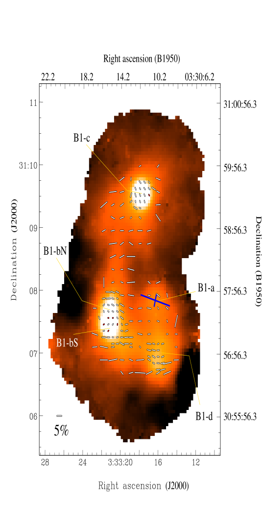
Figure 1: 850 µm polarization pattern toward the “main core” of Barnard 1 is overlaid on the Stokes’ $I$ map. The greyscale range is $-1\sigma$ to $3\sigma$. Polarization data were sampled at 3″ and have been binned to 6″ (approximately half the JCMT beamwidth of 14″) on the bright cores where signal-to-noise ($\sigma_{p}$) is high and 12″ in the fainter regions. All vectors are associated with Stokes’ $I$ values greater than 20% the B1-d peak flux, $\sigma_{p}>3$, and an uncertainty in polarization percentage, $dp$, $<1$%. Red vectors have polarization percentage, $p$, $<1$% and were not included in any analysis of the polarization pattern. The vectors are accurate in position angle to better than 10^∘. The peaks B1-a, B1-bN and B1-bS have been labeled according to the designations of Hirano et al. (1999). We have designated the other two peaks B1-c and B1-d. The position of IRAS 03301+3057 is marked in blue where the lines denote the extent of the uncertainty in the IRAS position. The mean polarization percentage of the plotted vectors is 3.6% with a standard deviation of 2.2%. Coordinates in J2000 and B1950 are shown.

Figure 1 illustrates the polarization pattern detected across the B1 “main core” region as identified in CS and NH₃ by Bachiller et al. (1990). The polarization data are plotted on a colored greyscale Stokes’ $I$ map estimated by summing together the fluxes detected at all waveplate positions. Table 2 contains the data (with $p>1$%) in tabular form. Four peaks are distinguishable, these are labelled B1-a to B1-d. B1-a and B1-b (N and S) follow the classification of Hirano et al. (1999) as identified in H¹³CO⁺ and 850 µm SCUBA emission. The presence of two sources within B1-b was confirmed by 3.0 mm observations with the Nobeyama interferometer (Hirano et al., 1999). NH₃ (1,1) and (2,2) emission was observed from peaks corresponding to B1-a, B1-b and B1-c by Bachiller et al. (1990). The B1-d 850 µm peak lies approximately 1′ south of the B1-a molecular peak (Bachiller et al., 1990) which is likely associated with IRAS 03301+3057 (marked by a blue cross on Figure 1). No ammonia emission is concentrated at the B1-d position (Bachiller et al., 1990), although a very low signal-to-noise peak exists near this position in the H¹³CO⁺ map of Hirano et al. (1999).

3.1 Polarization Position Angles

Polarized emission is detected both on the bright cores and in regions of lower column density between them. The degree of alignment across the region is evidence for the presence of ordered magnetic fields within the main core of the B1 cloud. The data in high intensity regions have been binned to 6″ sampling, while data in fainter regions are binned to 12″ to improve the signal-to-noise ratio. The distributions of polarizations associated with faint emission and bright emission are plotted separately on Figure 2.

The distribution for faint $I$ (dashed line) is approximately Gaussian. A fit to these data yields a mean of 91.3° with a distribution width of 19.0°. Polarization position angles are measured such that values increase east of north. A goodness of fit measure to the data yields $\chi^{2}_{red}=0.6$. The statistical mean of the distribution is 88.3° (east of north) with a standard deviation of 27.7°. The distribution of vectors in regions of bright emission, however, cannot be fit effectively by a Gaussian (or even a series of Gaussians). The solid line of Figure 2 shows several peaks, each of which corresponds roughly to one of the bright peaks. We have indicated the peak sampled on the distribution.

Therefore, the polarization pattern in the ambient cloud material around the cores is defined by a mean polarization direction where the vectors are distributed about 90° (east of north), while the cores each exhibit different mean position angles. The core B1-b shows systematic variation in position angle. The northern core has $<\theta>\sim 65$°, while the southern core exhibits $<\theta>\sim 120$°. The B1-c core has $<\theta>\sim 35$°, and the B1-d core peaks around 90° east of north, in alignment with the fainter material in the cloud. This could indicate that this core is not strongly differentiated from the ambient cloud yet.

On Figure 2, we have also plotted the position angles associated with the two peaks observed in the optical absorption polarization data of Goodman et al. (1990a), taking into account the 90^∘ offset expected for emission polarimetry. These positions ($55^{\circ}$ and 161^∘) are not coincident with any of the peaks in the 850 µm distribution, either at high or low intensity.

3.1.1 Correlations between Adjacent Vectors

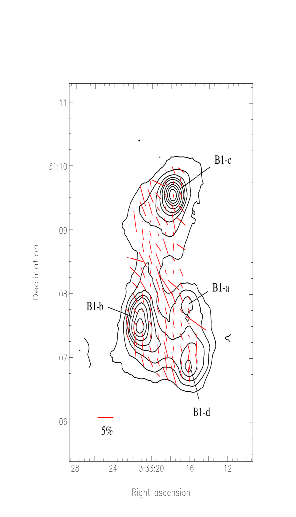
Figure 3: Core positions and the variation between neighbouring vectors. The positions of the cores are shown with contours of the Stokes’ $I$ emission. Contours plotted are: 0.2 to 1.0 Jy beam^-1 in steps of 0.2 Jy beam^-1, and 1.4 to 2.6 Jy beam^-1 in steps of 0.4 Jy beam^-1. (These correspond to visual extinction magnitude contours of 20 to 100 in steps of 20 magnitudes, and 140 to 260 in steps of 40 magnitudes.) We have compared each polarization vector shown in Figure 1 to its nearest neighbours in eight directions to a maximum radial separation of 17″. The data were then smoothed to 12″ sampling. The length of the vectors plotted is the mean change $\Delta p$ in the smoothed grid point, while the vector orientations indicate the mean change in direction $\Delta\theta$. Zero change in angle is indicated by 0^∘ (east of north). These data reveal that within cores, and between them, the position angles are strongly consistent, while the large vectors offsets from $0^{\circ}$ at the boundaries show where the changes in vector character occur. Coordinates are J2000.

To better examine the changes in the nature of the polarization data across the map, we have compared each vector to its closest eight neighbours, calculating the differences in polarization percentages and position angles for each pair of values. All the data of Figure 1 were used, except those values for which $p<1$% (shown in red). Next, the results were smoothed onto 12″ grid, by calculating the mean changes in polarization percentage and position angle. The resulting map is shown in vector form in Figure 3, where the vector magnitude is the mean change in polarization percentage in a grid unit and the vector angle is the mean change in orientation. No significant change in orientation is indicated by a vector at $0^{\circ}$ east of north.

Total intensity contours illustrate the positions of the cores on Figure 3. Only one peak is distinguishable in B1-b, but it is clear this core is elongated. As expected, the changes within the cores are relatively small. The position angles (and even polarization percentages) are consistent with relatively little change. Based on the histogram of the polarization data toward fainter regions shown in Figure 2, the vectors in this regime were also expected to be well aligned, and the data of Figure 3 show that this is indeed the case. The large variations in adjacent grid units are confined to the edge of the map and the boundaries between the B1-b and B1-c cores and the fainter material.

3.2 Continuum Fluxes Toward Cores in B1

Of the four dense cores detected in our polarization map, two have not been observed previously in continuum emission. These are B1-c and B1-d, although the latter may have been confused with B1-a in large beams (i.e., IRAS) particularly if they are at similar evolutionary stages. The brightest source in our map is B1-c, as revealed by the Stokes’ $I$ contours of Figure 3. We do not detect both peaks toward B1-b although Hirano et al. (1999) do in an earlier SCUBA map; their interferometic observation with the Nobeyama Millimeter Array clearly resolves two peaks toward this source. The slightly enhanced emission coincident with IRAS 03301+3057 is the faintest distinguishable peak at 850 µm. Table 3 summarizes the peak fluxes toward each of the four cores (for B1-b, the peak flux is that of B1-bS) and positions of these peaks.

For a cloud at a distance of 330 pc and assuming $\kappa_{850\micron}=0.01$ cm² g^-1, a mean molecular weight of 2.33 and a dust temperature of 20 K, we find that the column density $N(H_{2})=10^{23}S_{850}$[Jy beam^-1] cm^-2. The B1-c peak has a flux of 3 Jy beam^-1, which implies $N(H_{2})=3\times 10^{23}$ cm^-2, or 300 magnitudes of visual extinction. Toward B1-bS, we estimate $N(H_{2})=2.5\times 10^{23}$ cm^-2, which is within 50% of the estimate of Hirano et al. (1999). Assuming a core depth comparable to the FWHM of 30″ for B1-c yields a volume density of $2\times 10^{6}$ cm^-3 which is typical of prestellar and protostellar core densities.

3.3 Depolarization in Barnard 1

Figure 3 suggests that changes in polarization percentage are small within the cores of B1. The statistical means of the low intensity and high intensity vector populations are 4.5% and 2.6% in 81 and 74 values respectively. The standard deviations in these populations are 2.3% and 1.4%. In this case, the depolarization effect, declining polarization percentage with increasing intensity, may be weak within parts of B1. The easiest way of examining the depolarization effect is to plot $p$ versus $I$ for all vectors on the polarization map.

In Figure 4, we plot the data for the B1 region as presented in Figure 1 excluding only those data values with $p<1$% (plotted in red). The data exist in two populations, where the data at low intensities are binned to 12″ (shown as crosses) and the data at high intensities are binned to 6″ (shown as circles). Although these plots are shown in log-log space, the fits to the data were done to profiles of $p$ versus $I$ by minimizing $\chi^{2}$. This is a more effective treatment of the uncertainties since those for low values of $p$ are exaggerated in log space. The fits to these two populations produce completely consistent slopes, indicating that both can be characterized by power laws of the form: $p=AI^{\gamma}$ with an index of $\gamma\approx-0.8$. At high values of $I$ however, there is a slight thresholding of polarization percentage.

To better illustrate this, in Figure 5 we show the same style plot for three cores: B1-b (north and south combined), B1-c and B1-d. Vectors toward the cores B1-b and B1-c exhibit higher values of $p$ than expected given the declining trend below 1 Jy beam^-1. In fact, the distribution of $p$ versus $I$ flattens at high intensities. In the case of B1-b, this flattening could be the result of our lack of sensitivity to values of $p<1$%. However, for the B1-c core, this constraint removes only a single vector (which has a value of $0.99\pm 0.25$%). Thus, in B1-c, the depolarization effect does not follow the usual trend of declining polarization percentage as intensity increases. (The B1-d core does exhibit depolarization to its peak, which is significantly lower in intensity than B1-b and B1-c.) The B1-c core is well sampled (with only one vector missing) and definitely exhibits a flat dependence of $p$ on $I$ down to 30% of that core’s peak. The omitted vector (shown in red on Figure 1) does not correspond to the intensity peak of the core, but is associated with an intensity just 2/3 of the peak observed. To our knowledge, this is the first case of a bright core which does not exhibit depolarization over its whole observed intensity range. The observed threshold is not the effect of optical depth. We estimate that the optical depth at the B1-c peak is $\sim 0.015$ which is $<<1$.

4 Discussion

4.1 Interpreting the Polarization Pattern

Optical polarimetry using absorption of light from background stars was used to probe the magnetic field structure through dust at low extinctions in the Perseus cloud complex by Goodman et al. (1990a). They found a bimodal distribution of polarization vector orientations toward the complex such that the vectors lie roughly parallel and perpendicular to the major axis of $\sim 60^{\circ}$. They fit two Gaussians to their data set with means $71^{\circ}$ and $145^{\circ}$ east of north and 1 $\sigma$ dispersions of $12^{\circ}$ and $8^{\circ}$, respectively. Since there is no spatial distinction between the two populations and evidence in observations of molecular gas that two different clouds could lie along the same line of sight, they conclude that the two polarization populations are representative of two distinct clouds at different distances. The foreground cloud was predicted to have a low extinction ($A_{V}<1$ mag). Bimodal distributions in polarization vectors had been previously noted by studies toward the Perseus clouds NGC 1333 (Turnshek et al. (1980); Vrba, Strom & Strom (1976)) and Barnard 5 (Joshi et al., 1985).

In the process of generating an evolutionary model for the B1 cloud, Crutcher et al. (1994) adopt a mean plane-of-sky field direction along the minor axis of the Perseus (and hence B1) cloud which corresponds to the polarization distribution centered on $145^{\circ}$ east of north. In this case, the Goodman et al. (1990a) vectors centered on $71^{\circ}$ east of north would most likely be associated with the foreground cloud, at 200 pc distance (Cernicharo et al., 1985). If the interior of the dense B1 main core is threaded with the same field geometry as measured on the periphery of the B1/Perseus cloud, then a field of mean direction $145\pm 12^{\circ}$ should produce polarized emission from dust at a position angle of $55\pm 12^{\circ}$. Figure 2 demonstrates that there is no peak in the polarization data at 850 µm at $55^{\circ}$, although polarization vectors of B1-c and B1-bN fall roughly in the range of the optical polarization dispersion value. The second distribution measured by Goodman et al. (1990a) peaked at $71^{\circ}$, which corresponds to an emission polarization angle of $161^{\circ}$. Thus, there is no component of position angle in our data set which corresponds directly to either population of the optical polarization data. Hence, based on our emission polarimetry, which is believed to arise only in the regions of dense, cold dust, we cannot conclude which optical polarization direction is more likely associated with the Perseus complex.

4.1.1 Complete Depolarization of the Cores?

The polarization vectors across the B1-d peak are aligned with the faint emission polarization angles of $90^{\circ}$, but the brighter peaks, B1-b and B1-c, both exhibit different position angles. Given the previous observations of depolarization in bright peaks and the polarization plateau across these two cores, it would be tempting to think that the cores themselves are completely depolarized and that one might thus measure the polarization toward a different cloud along the line of sight at their positions. There are several reasons why this is unlikely to be the case.

In most well-sampled cores, depolarization is a non-linear function of intensity, so the polarization percentage rarely reaches zero (e.g. Henning et al. (2001); Ward-Thompson et al. (2000); Greaves et al. (1999); Greaves, Murray & Holland (1994); Minchin & Murray (1994)), and if it does become unmeasurably small, as it does at places in B1-b, then it does so at the highest intensities. Therefore, one might expect to see a varying position angle across cores that reflects the varying contribution of the core’s polarized intensity to the vector sum with the second cloud, revealing the second cloud’s position angle only toward the peak of the core. Furthermore, even in the case where the depolarization might atypically be complete across a core, this would effectively create a steeper than usual depolarization effect rather than a flat distribution of $p$ with $I$ as we particularly observe toward B1-c (see Figure 5). The reason is that if the polarized emission arose in a cloud other than B1 and were unassociated with the B1-c core (which we know to be in B1 through its associated molecular emission), the increasing contribution to the total intensity from the core (despite its contribution of zero polarized intensity) should produce a variation in $p$ with $I$ which varies exactly as the increase in intensity across the core. The only way this could be avoided would be if, as the intensity across the B1-c core increased, so did the polarized intensity in the second cloud. These increases would have to match each other exactly to produce the flat pattern we see. We dismiss this scenario as far-fetched.

In B1, we see not just a single core which exhibits a different position angle orientation than the ambient cloud, but instead there are two such cores, where B1-b includes systematic variation in $\theta$ from north to south. In order to see the optical polarizations from a foreground and background cloud in absorption, Goodman et al. (1990a) point out that the extinction of the nearer cloud must be low ($A_{V}\leq 1$ mag) or have significant fluctuations in order to see through to the background cloud. If the extinction in the cloud is on the order of 1 mag, then the cloud is not self-gravitating and hence is an unlikely source of 850 µm emission (and certainly 850 µm polarized emission, which is at most on the order of 10% of the total flux). This leaves the possibility of a denser cloud with significant fluctuations in column density across its projected surface.

The angular distance between the B1-b and B1-c cores is approximately 2 arcminutes. At a distance of 200 pc, which is the most probable location of a foreground cloud given previous molecular line observations, this corresponds to 0.12 pc, or about the scale of a self-gravitating core in a molecular cloud. Since we observe different position angles in the two bright cores (and a change in position angle within the B1-b core itself), this would suggest that fields of varying orientations are exhibited in the foreground fluctuations in the nearby cloud. This implies that the fluctuations in the foreground cloud are comparable to or smaller than the scale of a starless core. Since the two bright cores are associated with NH₃ emission (and hence known to be within the B1 cloud), the fluctuations would have to vary on an angular scale similar to the separation of cores in B1, despite being at a distance nearly a factor of two smaller. We conclude that attributing the polarization seen against the bright cores B1-b and B1-c to a foreground cloud suggests an unlikely configuration for a nearby cloud not detected in any dense tracers such as CS and NH₃.

However, the flattening of the $p$ versus $I$ relation in B1-c does suggest that this core is unusual in some way. Depolarization within cores is usually attributed to either changing grain or alignment physics with increasing density or varying (ordered or disordered) magnetic field geometry. It is possible that no stellar condensation has formed at the center of B1-c, in which case a field with a straight geometry may thread this core. Also, if no outflow is present, then theory suggests there should be no disk either, which means the field is unlikely to be tangled on small scales. Further study of this source to search for evidence of outflow or a protostellar condensation could provide some support for the suggestion that this is a starless core. However, this would not completely explain the pattern, since all the starless cores observed thus far with SCUBA do exhibit depolarization toward their intensity peaks (Ward-Thompson et al., 2000). The cores observed by Ward-Thompson et al. (2000) are all significantly closer than B1 (140-170 pc). The total flux from one of these cores (L183) is 2.8 Jy at 800 µm (Ward-Thompson et al., 1994). Therefore, cores of comparable brightness, both closer and further (i.e., LBS 23’s cores, Matthews, Fiege & Moriarty-Schieven (2002), hereafter Paper III) than B1, do exhibit depolarization to the highest intensities. The $p$ versus $I$ relation of B1-c is thus not easily explained purely by differing resolutions.

4.1.2 Polarization in Individual Cores

It is worth noting that the degree of alignment across the B1-a, B1-c, and B1-d cores is particularly strong. Figure 3 shows that these three cores are not significantly asymmetric, so the polarization patterns cannot be said to align with any preferred axes of the cores. The elongated core B1-b is the only one which exhibits systematic variation in polarization postion angle. Since this core is composed of two sources, the polarization patterns could be different within each core and then we observe their vector sum where the cores overlap.

Several models exist which predict the polarization patterns across cores depending on various physical interpretations. A recent publication by Padoan et al. (2001) predicts the continuum polarization for protostellar cores assembled via supersonic magnetized turbulent flows in models of molecular clouds. They find that the universally observed trend of declining polarization percentage with increasing intensity in star-forming cores can be reproduced by their model if grains are aligned only up to a threshold extinction ($A_{V}\sim 3$ mag in their simulation). Several of the resulting $p$ versus $I$ plots do suggest a flattening in the distribution at high values of intensity. However, one difference between their simulations (see Figs. 6 and 7 of Padoan et al. (2001)) and Figure 4 is the population of the bottom left quadrant (low $p$ and low $I$); vectors exist in this region in the simulations, whereas this region is devoid of vectors in Figure 4, despite complete sampling down to the intensity threshold. Measurement of low levels of polarized emission toward lower intensities will become possible with the next generation of detectors (e.g. SCUBA-2).

The fact that there is a potential for confusion between two clouds along the line of sight makes interpretation of the polarization data more complicated in Perseus. However, constraints on the column density and spatial scale of potential variations in extinction of a second cloud suggest that the overwhelmingly predominant source of polarized emission is the B1 cloud and its associated cores. The models of Padoan et al. (2001) and Fiege & Pudritz (2000) relate to cores forming from lower density, filamentary structures. B1 is not a significantly elongated cloud (although the Perseus complex itself appears elongated on very large scales), and its cores appear to be forming from density enhancements in its cold interior. A recent model of magnetized cores predicts a relation between the geometry of a core and the measured polarization position angles (e.g. Basu (2000)). However, the B1 cores are not significantly elongated; the only asymmetry is in B1-b, which is resolved into two sources with separate extended envelopes by Hirano et al. (1999).

4.2 An Estimate of the Total Field Strength and Direction in B1

Myers & Goodman (1991) describe a method by which the total field strength and direction can be estimated in a cloud toward which a series of independent Zeeman measurements of $B_{los}$ and polarization measurements to infer the orientation of $B_{pos}$ have been made. Their formalism is described for absorption polarimetry, but is easily adapted to emission polarimetry if simple assumptions are made about the relation between the orientations of polarization vectors and the plane-of-sky magnetic field.

A distribution of polarization data which can be fit by a single Gaussian is a good approximation to the precise function described in Myers & Goodman (1991) in the case where the nonuniform field is relatively small and the three dimensional random case can be assumed. As described in $\S$ 3.1 above, the polarization vectors associated with the faint lower density gas off the B1 cores can be fit with a single Gaussian distribution which has a mean of 91^∘ (east of north) and a width of 19^∘. At 12″ sampling, these vectors are not completely independent (since the JCMT beamwidth is 14″), but we use them to get a rough estimate of the field properties.

The Myers & Goodman model is based on the presence of both a uniform ($B_{0}$) and non-uniform ($B_{n}$) component to the field in the region. Non-uniform in this case refers to a disordered, possibly turbulent, field component (as opposed to an ordered, but not unidirectional field). Given a distribution of polarization data with mean polarization angle, $\Theta$, (in degrees) and dispersion, $s$, (in radians) and a series of Zeeman measurements with mean uniform component $\overline{B}_{0_{z}}$ and dispersion $\sigma_{B_{z}}$, the following quantities can be estimated: the inclination,

$$i=\arctan\left(\frac{\sigma_{B_{z}}}{s\overline{B}_{0_{z}}}\right);$$ (1)

the total uniform mean field strength,

$$B_{0}=\frac{\overline{B}_{0_{z}}}{\cos{i}};$$ (2)

and the dispersion in $\bf{B}$,

$$\sigma_{B}=\sigma_{B_{z}}N^{1/2}$$ (3)

where $N$ is the number of correlation lengths of the non-uniform field component through the cloud. The correlation length is an expression of how quickly the non-uniform component of the field changes through the depth of the cloud. Values of $B_{n}$ separated by less than a correlation length are likely to be correlated, while those more spatially separated than a correlation length are independent. Myers & Goodman (1991) derive the relation:

$$N_{max}=69\left(\frac{A_{V}}{\rm{mag}}\right)\left(\frac{B}{\mu\rm{G}}\right)^{-1}.$$ (4)

The maximum number of correlation lengths can be estimated under the assumption that the magnetic and gravitational energy densities are equal. Under this condition, $A_{V}/B\approx 0.17$ mag $\mu$G^-1, where $B$ is the total field strength (Chandrasekhar & Fermi, 1953; Myers & Goodman, 1988). This estimate yields $N_{max}\approx 12$.

The r.m.s. field strength and the relative strengths of the non-uniform to uniform magnetic field energy densities can then be calculated according to the relations:

$$<B^{2}>^{1/2}=\left(B_{0}^{2}+3\sigma_{B}^{2}\right)^{1/2};$$ (5)

and

$$\frac{M_{n}}{M_{u}}=\frac{3\sigma_{B}^{2}}{B_{0}^{2}}$$ (6)

where we have assumed a three-dimensional non-uniform field component.

We use the detection of $-27\pm 4$ $\mu$G toward the position of IRAS 03301+3057 (Goodman et al., 1989) as an estimate of the $B_{0_{z}}$ value. In the absence of other independent detections, there is no estimate of the dispersion in the line-of-sight field strength. Thus, we adopt a parameterized approach to combining the Zeeman and dust polarization data to estimate the three-dimensional field, where the ratio of $\sigma_{B_{z}}/B_{0_{z}}$ takes on a range of values (0.2, 0.4, 0.6 and 0.8). Table 4 then summarizes properties of the magnetic field in B1 based on equations (1), (2), (3), (5), and (6) for $N=1$ and $N=10$.

Finally, the direction of the uniform component of the magnetic field can be estimated:

$$\hat{B}_{0}=(\hat{N}\cos\Theta_{B}+\hat{E}\sin\Theta_{B})\sin i+\cos i\hat{z}.$$ (7)

For emission polarization data, we assume the mean magnetic field direction, $\Theta_{B}$, is related to $\Theta$ by $\pm 90^{\circ}$. Emission local to each dust grain should be related to the local field direction in this manner (Hildebrand, 1988), but for this to be the case in the vector averaged sum of all polarizations through the cloud (which is what we measure at the telescope) is to assume that the magnetic field orientation does not substantially vary through the depth of the cloud. This has been shown to be a poor assumption in some regions, where the polarization data support a more complex field geometry (i.e., OMC-3 in Orion A, Paper II; NGC 2024 in Orion B, Paper III; and NGC 2068, Paper IV). However, B1 is a dark cloud and not part of a giant molecular cloud complex like Orion; therefore, a uniform field structure (at least away from the cores) is not an unreasonable first-order assumption here. We note however that in utilizing this relation in B1, we are also assuming that all the polarized emission is arising in the B1 core, as opposed to in a second cloud as discussed above.

Using equation (7) and $\sigma_{B_{z}}/B_{0_{z}}=0.2$ (hence $i=31^{\circ}$ from the line of sight),

$${\bf B}_{0}=31\mu G\left[\pm(0.52\hat{N}+0.01\hat{E})-0.86\hat{z}\right].$$ (8)

We note that the direction of the field along the line of sight is toward the observer.

The field components can also be expressed in terms of two dimensions, $\hat{x}$ and $\hat{z}$, where $\hat{x}$ lies along the plane-of-sky mean field direction, as estimated from the mean polarization direction. In this case,

$$B_{0_{x}}=B_{0_{z}}\tan{i}$$ (9)

and substitution of $B_{0_{z}}$ and $i$ gives:

$${\bf B}_{0} = B_{0_{x}}\hat{x}+B_{0_{z}}\hat{z}$$ (10)

$$= \pm 19\ \mu\rm{G}\ \hat{x}-27\ \mu\rm{G}\ \hat{z}.$$ (11)

Based on comparisons with theoretical predictions based on the assumptions of equality of magnetic fields and kinetic energy and equivalence of magnetic and gravitational energies, Crutcher et al. (1993) found that the $\hat{z}$-field component measured in B1 agreed well with predicted values if the inclination of the field to the line of sight are close to zero. Furthermore, because B1 was the only cloud with a detected magnetic field out of 12 in their survey, there was a concern that B1 might have an atypically strong field. Based on statistical analysis, Crutcher et al. (1993) concluded that this need not be the case if the magnetic field in B1 lies nearly along the line of sight. The $B_{0_{z}}$ value of $-27\pm 4$ $\mu$G may be substantially higher than the magnetic field strength at locations away from the dense cores. Therefore, our analysis represents upper limits to the field strenghths in low column density gas.

However, our detection of ordered polarization vectors from dust associated with the main core of molecular gas in B1 indicates that at least some of the magnetic field in the region lies in the plane of the sky. Unfortunately, there is no way to unambiguously determine the plane-of-sky field strength from polarization data alone, since the degree of polarization may depend on grain size, shape, composition and degree of alignment or spin, as well as field strength (Hildebrand et al., 2000). We note that the OH Zeeman measurements can effectively probe regions with densities as high as $n(H_{2})\sim 10^{4}$ cm^-3 (Crutcher et al., 1994), quite comparable to the densities associated with the dust emission. Assuming a temperature of 20 K for the main core, the 850 µm flux density (at a level of 0.2 Jy) implies a column density of $N(H_{2})\sim 2\times 10^{22}$ cm^-2, which corresponds to a density of $n(H_{2})\sim 3\times 10^{4}$ cm^-3 if the emitting dust extends over the main core diameter of 0.8 pc (Bachiller et al., 1990). In reality, the emitting region of dust may be more confined along the line of sight, which would imply even higher densities. This is certainly the case where flux densities are high. The column density toward B1-c is $N(H_{2})\sim 3\times 10^{23}$ cm^-2. Since Zeeman data have been obtained toward regions of high density, it is possible that the OH Zeeman data and the dust emission polarimetry do not arise in precisely the same spatial regions of the cloud. They could, therefore, be sampling different field geometries, or at least different total field strengths. However, we have applied the Myers & Goodman (1991) method over a size scale comparable to the Arecibo beam at the frequency of the OH Zeeman measurements of Goodman et al. (1989), making our calculation quite reasonable for the lower column density dust.

5 Summary

We have detected polarized emission at 850 µm arising from the dense interior of the Barnard 1 dark cloud. Our observations are centered on the molecular “main core” observed by Bachiller et al. (1990), in which three ammonia peaks were identified. Submillimeter emission is detected coincident with each of the ammonia peaks. In total four dust cores are identified, one of which has been resolved into two sources (Hirano et al., 1999). Two of the dust condensations, B1-c and B1-d, have not been previously observed in continuum. The B1-a core is likely the 850 µm counterpart of IRAS 03301+3057. This source appears quite faint at long wavelengths. We note that the detection of two new dense dust condensations, plus the B1-b binary sources identified as young Class 0 sources by Hirano et al. (1999), increases the number of YSOs or pre-protostellar objects in B1 by almost a factor of 2. This indicates that the star formation efficiency in B1 is likely much larger than the 0.5% estimate by Bachiller et al. (1990) since there may be other as yet unobserved pre-protostellar or protostellar cores in the cloud of which we have observed only a fraction.

The polarized emission can be separated somewhat arbitrarily into two sub-groups by the coincident flux levels. Strong polarizations are measured toward faint dust emission regions where the mean polarization percentage is 4.5% (standard deviation 2.3%). The position angles are distributed about 90^∘ (east of north) and can be fit by a Gaussian of mean 91.3^∘ and dispersion $19^{\circ}$. The polarizations associated with high intensities (i.e., the cores) show smaller polarization percentages, with a mean of 2.6% and standard deviation 1.4%. The vectors show alignment across the cores, but each core does not exhibit the same mean position angle. A comparison of each vector to adjacent values shows that vectors are strongly aligned with their neighbours in position angle. The largest discrepencies are observed at the “boundaries” between the dense cores and the lower column density dust emission in which they are embedded.

Over the whole mapped area, we see evidence of the depolarization observed toward many star-forming cores. Interestingly, when the polarization percentages are plotted against intensity for individual cores, the $p$ versus $I$ relation flattens out at 30% and 40% of the peak emission from the B1-c and B1-b cores, respectively. The B1-c core exhibits only one vector with a value of $p<1$%, and thus the flattening in that core is real and not just an artifact of a lower limit on detectable polarizations or increasing optical depth. The observation of depolarization at the highest intensities of cores closer (Ward-Thompson et al., 2000) and further (Paper III) than B1 makes it unlikely that this effect is directly related to our resolution of B1 at 330 pc.

None of the orientations of polarization vectors measured by SCUBA are directly related to the two mean magnetic field directions detected with optical polarimetry of the Perseus complex (Goodman et al., 1990a). In the case where the B1 dense cores could be completely depolarized, the polarized emission along the line of sight to those cores would arise completely in the foreground cloud (proposed to be at 200 pc). If such a cloud contains fluctuations in extinction, those fluctuations must be on scales similar to the separation of cores in B1 at approximately half the distance. This is required to account for the differing orientations measured in the two bright cores, B1-b and B1-c. We dismiss this scenario as unlikely since, unless the polarized emission from the foreground cloud rises in such a way as to offset the increasing intensity toward the B1-c core peak, we should see a steeper depolarization toward B1-c than in typical cores, not the threshold we observe.

Finally, following the method of Myers & Goodman (1991), we have estimated the net field geometry in the B1 main core using our polarized emission data toward faint regions (centered on $90^{\circ}$ east of north) and the line-of-sight field strength toward B1 measured by Goodman et al. (1989). We find that the total uniform field component is described by:

$${\bf B}_{0}=31\mu G\left[\pm(0.52\hat{N}-0.01\hat{E})-0.86\hat{z}\right],$$

under the assumption of $\sigma_{B_{z}}/B_{0_{z}}=0.2$. The ratio of the magnetic energy of the non-uniform component of the field to the uniform component ranges from 0.09 to 0.9 for this case, depending on the number of correlation lengths of the non-uniform component through the cloud. This result is roughly consistent with the theoretical predictions based on virial and magnetic equilibrium in the cloud, for which the line-of-sight field was comparable to the total predicted field. The high degree of ordering in the polarization data itself suggests that some component (possibly a significant amount) of the magnetic field could lie in the plane of the sky.

Table 1: Observing Parameters for Jiggle Mapping of B1

Pointing Center		Number of
R.A. (J2000)	Dec. (J2000)	Times Observed
$03^{\rm h}33^{\rm m}$17$\fs$9	$+$31°09′32$\farcs$3	16
$03^{\rm h}33^{\rm m}$19$\fs$6	$+$31°08′28$\farcs$25	12
$03^{\rm h}33^{\rm m}$18$\fs$3	$+$31°07′03$\farcs$8	30

Note. — The chop throw used for all observations was 120″ at a chop position angle of 65^∘ (east of north).

Table 2: Barnard 1 850 µm Polarization Data

$\Delta$ R.A.	$\Delta$ Dec.	$p$	$dp$	$\sigma_{p}$	$\theta$	$d\theta$
(″)	(″)	(%)	(%)		(∘)	(∘)
Vectors associated with $I>$ 720 mJy beam-1
$-58.5$	$-136.5$	3.74	0.56	6.7	$-85.3$	4.3
$-64.5$	$-136.5$	5.24	0.83	6.3	$-78.3$	4.5
$-52.5$	$-130.5$	1.86	0.50	3.7	$68.1$	7.7
$-58.5$	$-130.5$	2.36	0.46	5.2	$85.0$	5.6
$-64.5$	$-130.5$	3.85	0.59	6.5	$-80.9$	4.4
$-70.5$	$-130.5$	9.06	0.76	11.9	$-80.6$	2.4
$-46.5$	$-124.5$	2.49	0.63	3.9	$67.3$	7.3
$-52.5$	$-124.5$	3.10	0.46	6.7	$64.0$	4.3
$-58.5$	$-124.5$	1.79	0.44	4.1	$85.4$	7.1
$-64.5$	$-124.5$	2.29	0.61	3.7	$-72.8$	7.6
$-46.5$	$-118.5$	4.10	0.52	7.9	$79.3$	3.6
$-52.5$	$-118.5$	3.68	0.41	9.0	$79.8$	3.2
$-58.5$	$-118.5$	2.25	0.43	5.2	$-87.8$	5.5
$1.5$	$-112.5$	2.50	0.51	4.9	$-89.0$	5.9
$-4.5$	$-112.5$	2.47	0.46	5.4	$-88.7$	5.3
$-10.5$	$-112.5$	4.79	0.43	11.0	$66.7$	2.6
$-16.5$	$-112.5$	4.52	0.48	9.5	$89.1$	3.0
$-22.5$	$-112.5$	1.74	0.50	3.5	$85.6$	8.2
$-46.5$	$-112.5$	4.25	0.55	7.7	$84.6$	3.7
$-52.5$	$-112.5$	2.25	0.47	4.8	$78.3$	6.0
$-58.5$	$-112.5$	1.46	0.48	3.0	$-66.1$	9.5
$-64.5$	$-112.5$	2.13	0.54	3.9	$-80.1$	7.3
$13.5$	$-106.5$	4.00	0.50	8.0	$89.8$	3.6
$7.5$	$-106.5$	2.59	0.35	7.5	$89.2$	3.8
$1.5$	$-106.5$	1.05	0.32	3.3	$81.9$	8.7
$-4.5$	$-106.5$	1.57	0.32	4.8	$-82.1$	5.9
$-10.5$	$-106.5$	2.75	0.38	7.2	$-86.7$	4.0
$-16.5$	$-106.5$	4.26	0.44	9.7	$-86.8$	3.0
$-22.5$	$-106.5$	3.99	0.43	9.3	$-89.1$	3.1
$13.5$	$-100.5$	1.28	0.32	4.0	$-80.5$	7.2
$-10.5$	$-100.5$	2.08	0.33	6.4	$83.2$	4.5
$-16.5$	$-100.5$	2.86	0.41	7.0	$-78.2$	4.1
$7.5$	$-94.5$	1.13	0.16	7.2	$-63.3$	4.0
$1.5$	$-94.5$	1.01	0.15	6.6	$-49.0$	4.4
$-10.5$	$-94.5$	1.28	0.36	3.5	$47.2$	8.1
$-16.5$	$-94.5$	2.53	0.45	5.6	$-82.8$	5.1
$19.5$	$-88.5$	2.38	0.41	5.8	$33.8$	4.9
$-4.5$	$-88.5$	1.18	0.24	5.0	$46.4$	5.8
$-10.5$	$-88.5$	3.40	0.41	8.4	$58.5$	3.4
$13.5$	$-82.5$	1.09	0.28	3.9	$28.0$	7.4
$7.5$	$-82.5$	1.15	0.18	6.5	$58.9$	4.4
$1.5$	$-82.5$	1.35	0.18	7.4	$67.5$	3.9
$-4.5$	$-82.5$	1.52	0.26	5.8	$68.0$	4.9
$-10.5$	$-82.5$	4.02	0.46	8.8	$66.9$	3.3
$13.5$	$-76.5$	1.53	0.37	4.1	$-50.2$	6.9
$7.5$	$-76.5$	1.50	0.22	6.8	$73.7$	4.2
$1.5$	$-76.5$	2.35	0.20	11.9	$66.6$	2.4
$-4.5$	$-76.5$	1.91	0.27	7.0	$71.2$	4.1
$-10.5$	$-76.5$	4.48	0.51	8.8	$65.5$	3.2
$13.5$	$-70.5$	3.00	0.64	4.7	$-80.1$	6.1
$7.5$	$-70.5$	4.50	0.37	12.1	$-87.4$	2.4
$1.5$	$-70.5$	1.98	0.28	7.2	$76.8$	4.0
$-4.5$	$-70.5$	1.35	0.34	3.9	$64.7$	7.3
$7.5$	$-64.5$	5.30	0.65	8.2	$87.8$	3.5
$1.5$	$-64.5$	4.13	0.45	9.3	$77.1$	3.1
$-4.5$	$-64.5$	2.98	0.51	5.9	$71.7$	4.9
$-28.5$	$13.5$	3.56	0.42	8.5	$61.2$	3.4
$-34.5$	$13.5$	1.25	0.37	3.4	$72.4$	8.4
$-22.5$	$19.5$	2.04	0.47	4.4	$-56.5$	6.5
$-28.5$	$19.5$	1.22	0.33	3.7	$9.7$	7.8
$-34.5$	$19.5$	1.41	0.25	5.6	$27.9$	5.1
$-40.5$	$19.5$	1.45	0.22	6.5	$19.8$	4.4
$-22.5$	$25.5$	3.12	0.43	7.2	$-24.0$	4.0
$-28.5$	$25.5$	2.62	0.31	8.3	$24.8$	3.4
$-34.5$	$25.5$	1.77	0.19	9.1	$31.6$	3.1
$-40.5$	$25.5$	1.69	0.17	9.9	$31.9$	2.9
$-28.5$	$31.5$	1.83	0.31	5.8	$30.0$	4.9
$-34.5$	$31.5$	1.34	0.18	7.4	$44.9$	3.9
$-40.5$	$31.5$	1.86	0.20	9.4	$47.0$	3.0
$-46.5$	$31.5$	1.88	0.30	6.3	$50.3$	4.5
$-52.5$	$31.5$	4.29	0.48	9.0	$64.6$	3.2
$-34.5$	$37.5$	2.15	0.29	7.4	$47.1$	3.9
$-40.5$	$37.5$	1.77	0.30	5.9	$46.9$	4.9
$-46.5$	$37.5$	1.58	0.38	4.1	$40.6$	6.9
Vectors associated with $I<$ 720 mJy beam-1
$-10.5$	$-139.5$	3.44	0.81	4.2	$47.8$	6.8
$-22.5$	$-139.5$	4.58	0.87	5.3	$-78.7$	5.5
$-34.5$	$-139.5$	11.66	0.93	12.6	$88.1$	2.3
$-46.5$	$-139.5$	6.88	0.52	13.2	$-70.8$	2.2
$-58.5$	$-139.5$	4.05	0.38	10.6	$-65.0$	2.7
$-70.5$	$-139.5$	8.00	0.64	12.4	$-73.1$	2.3
$13.5$	$-127.5$	8.54	0.96	8.9	$89.9$	3.2
$1.5$	$-127.5$	9.42	0.57	16.5	$-81.3$	1.7
$-10.5$	$-127.5$	3.99	0.41	9.7	$87.1$	3.0
$-22.5$	$-127.5$	3.64	0.44	8.2	$73.3$	3.5
$-34.5$	$-127.5$	8.27	0.45	18.5	$-86.2$	1.5
$-46.5$	$-127.5$	2.94	0.33	8.9	$67.2$	3.2
$-82.5$	$-127.5$	5.19	0.68	7.7	$-88.7$	3.7
$25.5$	$-115.5$	5.15	0.64	8.0	$-87.1$	3.6
$13.5$	$-115.5$	8.13	0.43	18.7	$82.0$	1.5
$1.5$	$-115.5$	2.91	0.30	9.6	$-85.2$	3.0
$-22.5$	$-115.5$	2.37	0.28	8.3	$84.0$	3.4
$-34.5$	$-115.5$	1.18	0.32	3.7	$56.5$	7.7
$-82.5$	$-115.5$	1.77	0.58	3.1	$86.0$	9.4
$25.5$	$-103.5$	6.52	0.46	14.1	$74.8$	2.0
$-34.5$	$-103.5$	4.63	0.31	15.1	$81.2$	1.9
$-46.5$	$-103.5$	2.64	0.30	8.7	$-85.3$	3.3
$-70.5$	$-103.5$	1.46	0.42	3.5	$-89.6$	8.2
$-82.5$	$-103.5$	2.14	0.63	3.4	$87.1$	8.4
$-22.5$	$-91.5$	3.11	0.31	10.2	$89.5$	2.8
$-34.5$	$-91.5$	3.41	0.36	9.4	$-87.3$	3.0
$-46.5$	$-91.5$	1.16	0.34	3.4	$84.4$	8.3
$-58.5$	$-91.5$	2.03	0.32	6.2	$79.1$	4.6
$-70.5$	$-91.5$	1.65	0.46	3.6	$22.2$	7.9
$-82.5$	$-91.5$	9.54	0.92	10.4	$-17.0$	2.7
$25.5$	$-79.5$	3.43	0.62	5.5	$88.8$	5.2
$-22.5$	$-79.5$	3.92	0.51	7.7	$75.4$	3.7
$-34.5$	$-79.5$	3.78	0.46	8.3	$-85.8$	3.4
$-46.5$	$-79.5$	4.09	0.36	11.5	$80.9$	2.5
$-58.5$	$-79.5$	1.67	0.32	5.3	$35.8$	5.5
$-70.5$	$-79.5$	3.06	0.43	7.2	$54.1$	4.0
$-10.5$	$-67.5$	3.89	0.31	12.7	$83.2$	2.3
$-22.5$	$-67.5$	6.48	0.62	10.5	$83.5$	2.7
$-46.5$	$-67.5$	2.37	0.41	5.7	$82.5$	5.0
$-58.5$	$-67.5$	4.19	0.33	12.8	$57.9$	2.2
$-70.5$	$-67.5$	3.29	0.49	6.7	$15.0$	4.3
$13.5$	$-55.5$	7.64	0.86	8.9	$0.1$	3.2
$1.5$	$-55.5$	2.23	0.43	5.2	$-76.8$	5.5
$-10.5$	$-55.5$	2.71	0.41	6.6	$70.5$	4.4
$-22.5$	$-55.5$	8.82	0.72	12.2	$-85.7$	2.3
$-46.5$	$-55.5$	3.04	0.98	3.1	$56.5$	9.2
$-58.5$	$-55.5$	4.43	0.81	5.4	$-72.3$	5.3
$1.5$	$-43.5$	2.54	0.72	3.5	$74.5$	8.1
$-10.5$	$-43.5$	2.53	0.59	4.3	$86.9$	6.7
$-22.5$	$-43.5$	7.08	0.90	7.8	$78.9$	3.7
$1.5$	$-31.5$	6.44	0.70	9.2	$-70.8$	3.1
$-10.5$	$-31.5$	5.43	0.59	9.1	$-67.9$	3.1
$-22.5$	$-31.5$	9.13	0.94	9.7	$90.0$	3.0
$1.5$	$-19.5$	8.57	0.79	10.9	$-84.0$	2.6
$-10.5$	$-19.5$	4.18	0.68	6.1	$-60.5$	4.7
$-22.5$	$-19.5$	4.86	0.79	6.1	$61.7$	4.7
$-34.5$	$-19.5$	2.73	0.67	4.1	$-84.6$	7.0
$-46.5$	$-19.5$	4.25	0.76	5.6	$-78.6$	5.1
$13.5$	$-7.5$	3.89	0.78	5.0	$-68.9$	5.7
$1.5$	$-7.5$	3.95	0.76	5.2	$-80.3$	5.5
$-10.5$	$-7.5$	3.63	0.58	6.3	$-89.6$	4.6
$-22.5$	$-7.5$	4.78	0.54	8.9	$-79.0$	3.2
$-34.5$	$-7.5$	4.93	0.45	11.0	$-88.6$	2.6
$-46.5$	$-7.5$	4.13	0.62	6.7	$-79.5$	4.3
$1.5$	$4.5$	4.15	0.74	5.6	$66.9$	5.1
$-10.5$	$4.5$	4.05	0.55	7.3	$-74.2$	3.9
$-22.5$	$4.5$	1.25	0.36	3.5	$-51.8$	8.2
$-34.5$	$4.5$	1.86	0.30	6.2	$54.0$	4.6
$-58.5$	$4.5$	7.14	0.87	8.2	$42.9$	3.5
$13.5$	$16.5$	8.55	0.93	9.2	$-58.2$	3.1
$1.5$	$16.5$	3.23	0.65	5.0	$-63.8$	5.8
$-10.5$	$16.5$	4.10	0.45	9.1	$-59.4$	3.2
$-58.5$	$16.5$	4.97	0.63	7.9	$-86.8$	3.6
$1.5$	$28.5$	7.91	0.73	10.8	$-84.6$	2.6
$-10.5$	$28.5$	4.22	0.47	9.0	$-77.2$	3.2
$-58.5$	$28.5$	3.48	0.43	8.0	$68.6$	3.6
$-10.5$	$40.5$	5.84	0.76	7.7	$-61.6$	3.7
$-22.5$	$40.5$	2.24	0.39	5.8	$-3.1$	5.0
$-58.5$	$40.5$	4.96	0.54	9.1	$72.1$	3.1
$-34.5$	$52.5$	2.08	0.69	3.0	$-71.1$	9.5
$-58.5$	$52.5$	2.88	0.72	4.0	$-47.1$	7.2

Table 3: Peak flux densities at 850 µm

Core	R.A.	Dec.	$S_{peak}$	Notes
	(J2000)	(J2000)	(Jy beam-1)
B1-a	$03^{\rm h}33^{\rm m}$16$\fs$4	$+$31°07′51″	0.68	IRAS 03301+3057 (B1-IRS)
B1-bS	$03^{\rm h}33^{\rm m}$21$\fs$3	$+$31°07′28″	2.5	Hirano et al. (1999)
B1-c	$03^{\rm h}33^{\rm m}$17$\fs$7	$+$31°09′31″	3.0	first continuum detection
B1-d	$03^{\rm h}33^{\rm m}$16$\fs$2	$+$31°06′49″	1.1	first continuum detection

Table 4: Magnetic Properties of Barnard 1

$\sigma_{B_{z}}$	$i$	$B_{0}$	$N$	$\sigma_{B}$	$<B^{2}>^{-1/2}$	Mn/Mu
($\mu$G)	(degrees)	($\mu$G)		($\mu$G)	($\mu$G)
5.4	31	31	1	5.4	32.4	0.09
			10	17.1	42.9	0.91
10.8	50	42	1	10.8	46.0	0.20
			10	34.2	72.6	2.00
16.2	61	56	1	16.2	62.6	0.25
			10	51.3	105	2.50
21.6	68	71	1	21.6	80.3	0.28
			10	68.4	138	2.80

Figure 2: Distributions of position angle in B1 are shown using histograms of the $\theta$ measured toward faint (dashed) and bright (solid) regions separately. The threshold used to discriminate between faint and bright regions was a Stokes’ $I$ value of 720 mJy beam^-1, as discussed in §3.2. The vectors associated with lower column densities exhibit a Gaussian distribution with a mean of $91^{\circ}$ and dispersion of $19^{\circ}$. The distribution of vectors toward the cores is not Gaussian, with each core dominating a different part of the total histogram. The position angles are labeled with the core dominating each peak. The dotted lines show the emission polarization position angles which correspond to the peaks observed in the Goodman et al. (1990a) distribution of optical absorption polarimetry (i.e., they are rotated by 90^∘).

Figure 4: Depolarization in regions of low and high column density. Polarization is plotted against intensity on a log-log scale for our two populations of vectors. Low column density data are plotted with crosses while circles illustrate vector magnitudes associated with the cores. The slopes derived from fits to the $p$ versus $I$ profiles yield the same power law index, $\gamma$ (where $p=AI^{\gamma}$), plotted as the slope on the logarithmic scale. We note, however, that despite the scatter in the plot, the vectors at higher intensities seem to flatten in $p$. This can be seen more clearly in Figure 5.

Figure 5: Depolarization toward individual cores. To better examine the change in polarization percentage at high intensities, we plot log $p$ versus log $I$ for individual cores. Essentially, we take all vectors around each core above the intensity threshold discussed in Figure 1. By plotting the three bright cores separately, it is clear that B1-b and B1-c show higher values of $p$ than expected given the slope of the relation below 1 Jy beam^-1. The threshold corresponds to $\sim 30$% of the peak of B1-c and $\sim 40$% of B1-b. In the text, we discuss possible systematic effects which could explain this flattening (i.e., the truncation of the data set below 1% and optical depth). We conclude that the threshold is a real effect for the B1-c core.

References

- André et al. (1993) André, P., Ward-Thompson, D., & Barsony, M. 1993, ApJ, 406, 122
- Bachiller & Cernicharo (1984) Bachiller, R., & Cernicharo, J. 1984, A&A, 140, 414
- Bachiller & Cernicharo (1986) Bachiller, R., & Cernicharo, J. 1986, A&A, 166, 283
- Bachiller et al. (1990) Bachiller, R., Menten, K.M., & del Rio-Alvarez, S. 1990, A&A, 236, 461
- Basu (2000) Basu, S. 2000, ApJ, 540, 103
- Bohlin, Savage & Drake (1978) Bohlin, R.C., Savage, B.D., & Drake, J.F. 1978, ApJ, 224, 132
- Borgman & Blaauw (1964) Borgman, J., & Blaauw, A. 1964, Bull. Astron. Inst. Netherlands, 17, 358
- Chandrasekhar & Fermi (1953) Chandrasekhar, S., & Fermi, E. 1953, ApJ, 118, 113
- Cernicharo et al. (1985) Cernicharo, J., Bachiller, R., & Duvert, G. 1985, A&A, 149, 273
- Cohen & Kuhi (1979) Cohen, M., Kuhi, L.V. 1979, ApJS, 41, 743
- Coppin et al. (2000) Coppin, K.E.K., Greaves, J.S., Jenness, T., & Holland, W.S. 2000, A&A, 356, 1031
- Crutcher (1999) Crutcher, R.M. 1999, ApJ, 520, 706
- Crutcher et al. (1994) Crutcher, R.M., Mouschovias, T.Ch., Troland, T.,H., & Ciolek, G.E. 1994, ApJ, 427, 839
- Crutcher et al. (1993) Crutcher, R.M., Troland, T.H., Goodman, A.A., Heiles, C., Kazès, I., & Myers, P.C. 1993, ApJ, 407, 175
- Draine & Weingartner (1996) Draine, B.T., & Weingartner, J.C. 1996, ApJ, 470, 551
- Fiege & Pudritz (2000) Fiege, J.D., & Pudritz, R.E. 2000, ApJ, 534, 291
- Goodman et al. (1989) Goodman, A.A., Crutcher, R.M., Heiles, C., Myers, P.C., & Troland, T.H. 1989, ApJ, 338, L61
- Goodman et al. (1990a) Goodman, A.A., Bastien, P., Myers, P.C., & Ménard, F. 1990a, ApJ, 359, 363
- Goodman et al. (1990b) Goodman, A.A., Myers, P.C., Bastien, P., Crutcher, R.M., Heiles, C., Kazès, I., & Troland, T.H. 1990b, in Galactic and Intergalactic Magnetic Fields, eds. Beck, R. et al. , IAU, 140, 319
- Greaves et al. (2002) Greaves, J.S., Holland, W.S., Jenness, T., Moriarty-Schieven, G., Chrysostomou, A., Berry, D.S., Murray, A.G., Nartallo, R., Ade, P.A.R., Gannaway, F., Haynes, C.V., Tamura, M., Momose, M., & Morino, J.-I. 2002, MNRAS, submitted
- Greaves et al. (1999) Greaves, J.S., Holland, W.S., Minchin, N.R., Murray, A.G., & Stevens, J.A. 1999, A&A, 344, 668
- Greaves et al. (2000) Greaves, J.S., Jenness, T., Chrysostomou, A.C., Holland, W.S., & Berry, D.S. 2000, in Imaging at Radio through Submillimeter Wavelengths, eds. J.G. Mangum & S.J.E. Radford, ASP-CS 217, 18
- Greaves, Murray & Holland (1994) Greaves, J.S., Murray, A.G., & Holland, W.S. 1994, A&A, 284, L19
- Henning et al. (2001) Henning, Th., Wolf, S., Launhardt, R., & Waters, R. 2001, ApJ, 561, 871
- Hildebrand (1988) Hildebrand, R.H. 1988, QJRAS, 29, 327
- Hildebrand et al. (2000) Hildebrand, R.H., Davidson, J.A., Dotson, J.L., Dowell, C.D., Novak, G., & Vaillancourt, J.E. 2000, PASP, 112, 1215
- Hirano et al. (1999) Hirano, N., Kamazaki, T., Mikami, H., Ohashi, N., & Umemoto, T. 1999, in Star Formation 1999, 181
- Hirano et al. (1997) Hirano, N., Kameya, O., Mikami, H., Saito, S., Umemoto, T., & Yamamoto, S. 1997, ApJ, 478, 631
- Jenness, Lightfoot & Holland (1998) Jenness, R., Lightfoot, J.F., & Holland, W.S. 1998, Proc. SPIE, 3357, 548
- Joshi et al. (1985) Joshi, U.C., Kulkarni, P.V., Bhatt, H.C., Kulshrestha, A.K., & Deshpande, M.R. 1985, MNRAS, 215, 275
- Lang & Willson (1979) Lang, K.R., & Willson, R.F. 1979, ApJ, 227, 163
- Lynds (1969) Lynds, B.T., 1969, PASP, 81, 496
- Matthews, Fiege & Moriarty-Schieven (2002) Matthews, B.C., Fiege, J.D., & Moriarty-Schieven, G. 2002, ApJ, in press (Paper III)
- Matthews & Wilson (2002) Matthews, B.C., & Wilson, C.D. 2002, ApJ, accepted (Paper IV)
- Matthews, Wilson & Fiege (2001) Matthews, B.C., Wilson, C.D., & Fiege, J.D. 2001, ApJ, 562, 400 (Paper II)
- Minchin & Murray (1994) Minchin, N.R., & Murray, A.G. 1994, A&A, 286, 579
- Myers & Goodman (1988) Myers, P.C., & Goodman, A.A. 1988, ApJ, 326, L27
- Myers & Goodman (1991) Myers, P.C., & Goodman, A.A. 1991, ApJ, 373, 509
- Onishi et al. (1998) Onishi, T., Mizuno, A., Kawamura, A., Ogawa, H., & Fukui, Y. 1998, ApJ, 502, 296
- Padoan et al. (2001) Padoan, P., Goodman, A.A., Draine, B., Juvela, M., Nordlund, Å., & Rögnvaldsson, Ö. 2001, ApJ, 559, 1005
- Padoan & Nordlund (1999) Padoan, P., & Nordlund, Å. 1999, ApJ, 526, 279
- Purcell (1979) Purcell, E.M. 1979, ApJ, 231, 404
- Sargent (1979) Sargent, A.I., 1979, ApJ, 233, 163
- Turnshek et al. (1980) Turnshek, D.A., Turnshek, D.E. & Craine, E.R. 1980, AJ, 85, 1638
- Vrba, Strom & Strom (1976) Vrba, F.J., Strom, S.E., & Strom, K.M. 1976, AJ, 81, 958
- Ward-Thompson et al. (2000) Ward-Thompson, D., Kirk, J.M., Crutcher, R.M., Greaves, J.S., Holland, W.S., & André, P. 2000, ApJ, 537, 135
- Ward-Thompson et al. (1994) Ward-Thompson, D., Scott, P.F., Hills, R.E., & André, P. 1994, MNRAS, 268, 276