The small-scale structure of the Magellanic Stream

Abstract

We have mapped two regions at the northern tip of the Magellanic Stream in neutral hydrogen 21-cm emission using the Arecibo telescope. The new data are used to study the morphology and properties of the Stream far away from the Magellanic Clouds, as well as to provide indirect constraints on the properties of the Galactic Halo. We investigate confinement mechanisms for the Stream clouds and conclude that these clouds cannot be gravitationally confined or in free expansion. The most likely mechanism for cloud confinement is pressure support from the hot Galactic Halo gas. This allows us to place an upper limit on the Halo density: $n_{\rm h}(15~{}{\rm kpc})=10^{-3}$ cm^-3 and/or $n_{\rm h}(45~{}{\rm kpc})=3\times 10^{-4}$ cm^-3 depending on the distance. These values are significantly higher than predicted for an isothermal stratified Halo.

1 Introduction

The Magellanic Stream (MS) is a thin, $\sim$ 10^∘ wide (Putman & Gibson, 1999), tail of neutral hydrogen (HI), emanating from the Magellanic Clouds (MCs: the Large Magellanic Cloud, LMC, and the Small Magellanic Cloud, SMC) and trailing away for almost 100^∘ across the sky ($-60$^∘$<$ Dec $<+15$^∘). This huge HI structure is the most fascinating signature of the wild past interaction of our Galaxy with the MCs, and the MCs with each other. At the same time, streaming so far away from the MCs into the Galactic Halo, the MS is an excellent probe of the properties of the outer Galactic Halo, for which otherwise we have very few observational clues.

For many years the MS was viewed as a complex of six discrete concentrations (Mathewson et al., 1974). The new HI Parkes All-Sky Survey (Putman & Gibson 1999) reveals the more complex nature of the MS, with a fascinating network of filaments and clumps. No stars have been found so far in the MS, making it the closest medium to a primordial environment that exists in the Local Group today.

H_α emission appears to be routinely detected throughout the MS (Weiner et al., 2002), suggesting that the MS is being ionized by photons escaping from the Galaxy (Bland-Hawthorn & Maloney, 1999). While this mechanism is in accord with the H$\alpha$ observations of many high velocity clouds (HVCs), the predicted H$\alpha$ flux for the MS is significantly lower than what is found observationally (Weiner et al., 2002; Bland-Hawthorn & Maloney, 2002), suggesting that an additional source of ionization must be invoked. Several possible mechanisms have been suggested, including an interaction between the MS gas and the hot Galactic Halo gas, turbulent mixing, the existence of young massive stars embedded in the MS (Bland-Hawthorn & Putman, 2001), shocks, self-interaction of the MS gas, and magnetic fields (Konz et al., 2001).

The MS appears to be the result of interaction between the Galaxy and the MCs, but there is no consensus as to the exact form of this interaction (Putman, 2000b). Theories have swung back and forth on the relative importance of tidal stripping (Murai & Fujimoto, 1980; Gardiner & Noguchi, 1996) and various kinds of gas dynamical interactions (Mathewson et al., 1987). The recent discovery by Putman et al. (1998) of a counter HI stream, leading the MCs, lends weight to the tidal origin theory.

The work presented in this paper was motivated by the following two questions.

(1) Is the MS dissipating into the Halo?
The most fundamental issue about the origin and structure of the MS is to what extent interaction with the Galactic Halo determines or influences the MS gas. This problem becomes particularly important at the extreme northern end of the MS, because without pressure from an external medium the MS clouds should dissipate on a short time scale. However, if the external pressure is sufficient to confine the MS clouds, then the gaseous Galactic Halo has a much higher scale height than most theories predict. This paper addresses several issues in relation to this particular question.

(2) Is a hierarchy of structures present in this almost primordial environment?
In the Galaxy, a hierarchy of structure is present in the diffuse interstellar medium (ISM), down to very small scales. This is mainly ascribed to interstellar (IS) turbulence. This process is seen both in the ionized medium, traced by pulsar scintillation and dispersion variations, and in the atomic gas, traced by the spatial power spectrum of HI emission and absorption fluctuations (Fiedler et al., 1994; Green, 1993; Lazarian & Pogosyan, 2000; Dickey et al., 2001). Recently it has become possible to extend these studies to other galaxies, at least to our neighbors (Westpfahl et al., 1999; Stanimirovic et al., 1999; Elmegreen et al., 2001). The results suggest that the processes we see at work in the solar neighborhood are quite general. As the IS turbulence is driven, at least partially, by stellar processes such as winds and supernova remnants, it would be quite a surprise if the same turbulence spectrum was seen in an environment without any stars at all, like the MS. We have addressed this question briefly in Stanimirovic et al. (2002) and will concentrate on it further in a subsequent paper.

This paper is organized as follows: In Section 2 we summarize previous HI observations of the MS, and especially its northern part. As parameters such as the MS age and its distance come up often throughout this paper, a brief description of various theories for the MS formation is also outlined here. Section 3 describes new HI observations of two regions at the tip of the MS conducted with the Arecibo telescope. The HI data and observational results obtained are presented in Section 4. Several clumps and their properties are shown in Section 5. In Section 6 we discuss clump confinement issues and the constraints they place on the density of the Galactic Halo. Expected Halo densities, as well as several theoretical approaches for considering interactions between an MS cloud and the ambient medium, are discussed. An alternative explanation for the velocity field of one of the regions is also presented. We summarize our results in Section 7.

2 Previous HI observations and theoretical models

Figure 1: [f1.jpeg] The HI distribution of the MS from Mathewson & Ford (1984) is shown in the upper panel. The lower panel shows clouds MS III through MS VI of the MS as seen by the Parkes HIPASS survey (Putman et al. 2002). The two regions observed with the Arecibo telescope and presented in this paper are outlined with dashed lines.

2.1 Lower resolution observations

First HI detections of the MS were obtained by Dieter (1965) and Wannier & Wrixon (1972), however Mathewson et al. (1974) were the first to discover a coherent large-scale structure which they named the Magellanic Stream. Observations with better resolution and sensitivity followed by Cohen & Davies (1975), Mirabel et al. (1979), Erkes et al. (1980), Mirabel (1981) and Mathewson & Ford (1984). These observations revealed the large-scale morphology of the MS, that is traditionally viewed as a long filament, containing a bead-like sequence of six discrete clouds: MS I, near the MCs at Dec $\sim-60$^∘, to MS VI at the very northern tip at Dec $\sim+15$^∘ (Mathewson et al., 1977), see the top panel in Fig. 1. Mirabel (1981) in particular focused on the tip of the MS, searching for evidence of its disintegration. Wayte (1989) used the Parkes 64-m dish to uncover complex and chaotic motions right at the MS tip.

The most recent HI observations of the MS, with spatial resolution of 15 arcmin and velocity resolution of 26 km s^-1, were undertaken with the Parkes Multibeam system (Putman, 2000b; Putman et al., 2002). These, as well as the recent observations obtained with the same instrument but with higher velocity resolution of 1 km s^-1 by Brüns et al. (2000), revolutionized the classical picture of the MS. Instead of six concentrations of gas, two striking, long and distinct filaments are seen that run together for most of the length of the MS but merge in several places, giving the appearance of a double-helix structure. North of Dec $\sim 0$^∘, the two filaments break into a network of clumps and smaller filaments (see the bottom panel in Fig. 1). A global velocity gradient is observed along the MS, from $\sim+350$ km s^-1 (LSR) near the MC’s to $\sim-450$ km s^-1 (LSR) at the very northern tip.

2.2 Theoretical models

The two leading hypotheses for explaining the origin of the MS are based on tidal interaction versus ram pressure stripping, and are applied in several models. These two families of models predict different ages and distances for the MS. As the predicted parameters are important for the calculations in Sections 5 and 6 we carry out calculations for both sets of model predictions.

The tidal hypothesis (Murai & Fujimoto, 1980; Lin & Lynden-Bell, 1982; Gardiner et al., 1994; Gardiner & Noguchi, 1996; Yoshizawa & Noguchi, 1999) — invokes the idea of gravitational stripping of the SMC gas by the Galaxy. According to N-body simulations, the MS was formed 1.5 Gyr ago in a tidal encounter between the LMC and the SMC at their perigalactic passage. This encounter drew gas out of the SMC that later evolved into a leading bridge and a trailing tail. The MS follows the MCs on an almost polar orbit with a transverse velocity of 220 km s^-1 (LSR). Simulations show that the MS gas occupies a range of distances, from 45 kpc in the vicinity of MS III, to 60 – 70 kpc at MS VI.

One of the main drawbacks of the tidal model used to be the observation of only one tail of gas behind the MCs. Recent Parkes observations (Putman et al., 1998) have discovered the ‘Leading Arm Feature’ (LAF), a counter-stream that leads the direction of motion of the MCs, as expected in the tidal models. The absence of stars in the MS is another troubling issue for tidal models, as both stars and gas should be affected equally by tides. However, the most recent N-body simulations by (Yoshizawa & Noguchi, 1999) show that a very compact initial configuration of the SMC stellar disk could result in only gas being disrupted, while the stars are left unaffected.

The ram-pressure hypothesis (Moore & Davis, 1994; Heller & Rohlfs, 1994; Sofue, 1994) — invokes the idea of ram-pressure stripping of gas from the MCs by an extended halo of diffuse gas around the Galaxy. Here, the MCs entered the extended ionized halo of the Galaxy some 500 Myr ago at a galactocentric distance of 65 kpc. Material was then stripped from the SMC and the intercloud region and began to fall toward the Galaxy. In this model, the gas with the lowest column density, that lost the most orbital angular momentum, has fallen the furthest toward the Galaxy. This gas is currently located at the tip of the MS, at a galactocentric radius of 25 kpc. The model requires that the diffuse Galactic Halo has densities of $\sim 5\times 10^{-5}$ cm^-3 at distance of 65 kpc in order to strip gas, but not decelerate it too much.

The tidal $+$ drag model (Gardiner 1999; Moore & Davis, in preparation) The recent observational confirmation of the LAF provides a new set of parameters for theoretical models. In order to better constrain the observational characteristics of the LAF, Gardiner (1999) introduced a weak non-gravitational term (a drag term) into the classical tidal model. The new simulations show interesting results: while the LAF is reproduced, simulated particles form a complete ring from the LAF, connecting the LAF to two trailing streams. These streams have different galactocentric velocities starting from MS I to MS V, and then meet together again around MS VI (see Fig. 4 from Gardiner 1999). This simulation predicts that large-scale velocity splitting should be seen throughout most of the MS. The success of this model, based on both gravitational and non-gravitational forces, encourages further developments in the field that are eagerly anticipated (Moore, in preparation; Maddison, Kawata, & Gibson 2002).

3 Observations and data reduction

The observations were obtained with the 305-m Arecibo telescope in June and July of 2000 and June of 2001. The Gregorian feed was used with the narrow 21-cm (L-band) receiver. The illuminated part of the 305-m dish covers an area of about 210$\times$240 m, giving a beam FWHM of approximately 3^′.1 $\times$ 3^′.4 arcmin (Heiles et al., 2001). Two observing bandwidths of 12.5 and 6.25 MHz were used simultaneously on two correlator boards, each with 1024 channels, for each circular polarization. The resultant velocity resolution is 2.6 and 1.3 km s^-1, respectively.

Data were taken in the on-the-fly mapping mode, by driving in RA, at a rate of 4 arcsec per sec, and stepping in Dec by 2 arcmin between strips. The correlator was set to make one scan per strip by recording data continuously every 30 sec, which is effectively every 2 arcmin on the sky. As a result the data were slightly undersampled. At the beginning of each scan, a noise diode of known temperature was fired for 3 sec for calibration.

Two regions of interest were selected from Mirabel et al. (1979): one centered at the northern tip of the MS, $(l,b)=(86.7,-42.8)$, and the other in the MS V region, $(l,b)=(94.4,-50.6)$ (Fig. 1, these regions are outlined in the lower panel). Below we refer to these areas as MS VI and MS V, with the understanding that our maps do not cover the full extents of those clouds. Both regions were mosaiced with many small, overlapping maps, each of 10$\times$10 arcmin, which take $\sim$ 1 h to observe. The mosaic pieces were combined during the gridding process.

We removed a linear baseline by fitting ranges of emission-free channels on both sides of the line. The gain correction, as a function of both azimuth and zenith angle, was then applied. All spectra were subsequently convolved onto a sky grid using a Gaussian convolution function with FWHM of 2.6 arcmin, broadening the angular resolution to $\sim$ 4 arcmin. A gridding correction factor of 1.45 (Sramek & Schwab, 1989) was applied to account for the new beam size (S. Stanimirovic 2002, in preparation).

The relationship between flux density and brightness temperature is given by $S({\rm Jy~{}beam^{-1}})=0.11T_{\rm b}(\rm{K})$. The noise level is 0.04 K per 1.3 km s^-1 wide channel, which is equivalent to a column density of $\sim$ 10¹⁷ cm^-2. The peak brightness temperature is 1.5 K in the MS VI region, and 1.1 K in MS V. For comparison, Mirabel et al. (1979) obtained a maximum column density of $\sim$ 4$\times$10¹⁹ cm^-2 in the MS VI region using the Jodrell Bank telescope. In the same region we derive a maximum column density of 4.3$\times$10¹⁹ cm^-2.

4 Observational Results

4.1 Morphology and velocity field of the MS VI region

Figure 2: [f2.jpeg]The RA–Dec images of the MS VI region for different LSR velocities given in the top-left corner. The grey-scale intensity range is $-0.05$ to 0.3 K with a linear transfer function.

Figure 3: [f3.jpeg] Position–velocity diagrams of the MS VI region taken at different Dec values, given in the top-left corner. The grey-scale intensity range is 0.05 to 0.7 K with a linear transfer function.

Figure 4: [f4.jpeg](a) An HI column density image of MS VI overlaid with contours. The grey-scale range is 0 to 2.4$\times 10^{19}$ cm^-2. Contour levels are from 7 to 30$\times 10^{18}$ cm^-2, with a contour step of 6$\times 10^{18}$ cm^-2. The maximum column density is 3.9$\times$ 10¹⁹ cm^-2 at RA 23^h 07^m 52^s, Dec 11^∘ 31^′ 28^′′. (b) The first moment map of the MS VI region overlaid with contours. Contours range from $-400$ to $-360$ km s^-1, with a step of 10 km s^-1. The grey-scale range is $-391$ to $-364$ km s^-1 with a linear transfer function. Two prominent velocity ridges are shown with dashed lines: the east ridge with a mean velocity of $-397$ km s^-1, indicated with points labeled with A and B; the west velocity ridge with a mean velocity of $-370$ km s^-1, indicated with points labeled with C, D and E. An increase in noise toward map edges is noticeable.

The MS VI data is shown in Fig. 2 where several velocity channels through the spectral-line data cube are presented. Fig. 3 shows position-velocity cuts. Fig. 4 shows maps of the HI column density and the intensity-weighted velocity field (panels a and b). This region has several elongated clumps, inter-connected and forming a long curved filament. Often, sub-clumps are found nested inside larger clumps. We identify individual clumps and describe their properties in Section 5.1. Several interesting features appear in the data.

A large loop-like feature, centered at RA 23^h 07^m 26^s, Dec 12^∘47^′ 30^′′, with radius of 50 arcmin, is visible between $v_{\rm LSR}=-360$ and $v_{\rm LSR}=-385$ km s^-1. The loop is present through $\sim$15 velocity channels but its size appears to stay the same from channel to channel. Although at first glance this loop is reminiscent of HI holes associated with expanding shells of gas seen in many galaxies, because no systematic change of the radius with velocity is found this cannot be interpreted as an expanding shell. Velocity profiles along the loop are broad but always single peaked.

It is interesting to note that the most prominent clumps have a dominant orientation, from south-west to north-east, with position angle of $\sim-40$^∘ (measured counter-clock wise from north). This corresponds to a position angle of $\sim 90$^∘ in the Magellanic coordinate system, defined by Wakker (2001) and is parallel to the main axis of the MS (Putman, 2000a). Similar orientation of clumps in MS VI was noted previously by Mirabel et al. (1979).

The total HI mass in the mapped region is 3.7$\times$ 10⁵ M_⊙, if the distance of 60 kpc is assumed, and it comprises about 28% of the HI mass in the whole MS VI region estimated by Putman (2000a).

The velocity profiles in this region are single-peaked but quite broad with the dispersion being $\sim$ 15 km s^-1. Several RA-velocity diagrams are shown in Fig. 3. At about Dec 13^∘05^′ an interesting velocity gradient of almost 40 km s^-1 (LSR) is obvious. This gradient stays almost the same in the galactocentric velocity system, meaning that a spatial variation of the projection of the LSR velocity relative to the Galactic Center cannot explain the velocity field in this relatively small, 40$\times$40 arcmin, field.

The velocity field shown in Fig. 4 is the first moment map of the HI cube. The two prominent features in this map are north-south ridge-lines at velocity $-365$ to $-375$ km s^-1 in the east, and velocity $-395$ to $-400$ km s^-1 in the west. The points labeled A and B in Fig. 4 indicate the extent of the east ridge which may continue beyond the edge of our map. Points labeled C, D and E indicate the extent of the west ridge. The steep velocity gradient evident in the middle panels of Fig. 3 is in the region bounded by points A, B, C and D in Fig. 4. This region alone resembles the velocity pattern of a rotating disk, however the velocity field of the larger area does not fit this interpretation. We discuss this further in Section 6.6.

The velocity field in Fig. 4 is most likely caused by a combination of blending of smaller clumps along the line of sight and an interaction between the MS clouds and the ambient medium. With the Arecibo beam we are able to resolve several clumps blended together and forming a velocity gradient, see Fig. 3, especially around Dec 13^∘ 08^′. Some of these clumps show tails in velocity and sharp edges. This may be due to interaction with the surrounding medium. We discuss clump morphology in Section 6.7. Mirabel et al. (1979) saw a similar phenomenon in another MS VI region, while Wayte (1989) attributed broad velocity profiles to the breaking of the MS clouds into sub-clouds with different velocities.

4.2 Morphology and velocity field of the MS V region

Velocity channel maps presented in Fig. 5 show the general morphology of the MS V region. Several dominant large-scale features are visible. In the $-320$ km s^-1 plane there is a round cloud centered around RA 23^h 39^m, Dec 07^∘35^′ 00^′′. This region shows single-peaked velocity profiles. A long, straight filament stretches north-south for almost one degree, at RA 23^h 38^m 30^s from Dec 8^∘ to 9^∘, at velocity of $\sim-327$ km s^-1. At higher velocities of $-340$ to $-355$ km s^-1, the most prominent feature is a curved filament, centered at RA 23^h 39^m 30^s, Dec 07^∘40^′. This consists of a core superposed on an arc that extends for almost 1.3^∘.

North of Dec = 07^∘20^′ all line profiles show double peaks. This is shown in the position-velocity diagrams, Fig. 6, where a single velocity component is present only in the upper left panel. All other panels show double profiles. The two velocity peaks are roughly centered at $\sim-320$ and $\sim-360$ km s^-1 and run almost in parallel.

Double-peaked velocity structure has been seen previously in MS V by Mirabel et al. (1979) at very similar central velocities. Wayte (1989) also noted this velocity bifurcation in several regions in the MS. The most recent HIPASS data, with very coarse velocity resolution of about 26 km s^-1, show that spatially different filaments are common throughout the whole MS and most likely have different origins (Putman, 2000a). Similar line-splitting is found in several compact HVCs by Braun & Burton (2000), who suggest that this structure is caused by organized outflows or inflows.

Figure 5: [f5.jpeg]The RA–Dec images of the MS V region for different LSR velocities given in the top-left corner. The grey-scale intensity range is $-0.01$ to 0.9 K with a linear transfer function.

Figure 6: [f6.jpeg]Position–velocity diagrams of the MS V region taken at different Dec values, given in the top-left corner. The grey-scale intensity range is 0 to 1.3 K with a linear transfer function.

What causes the dual velocity structure seen in MS V? The velocity separation between the two peaks of $\sim 40$ km s^-1 is reminiscent of velocity features seen in the SMC. This was formerly interpreted as a signature of the SMC being ripped into two clouds which began during its last close encounter with the LMC some 200 Myr ago (Mathewson & Ford 1984). Recently, high spatial and velocity resolution observations of the SMC (Staveley-Smith et al., 1997; Stanimirovic et al., 1999) discovered more complex velocity profiles and numerous expanding shells of gas. This line-splitting in the SMC is now attributed primarily to the effect of expanding shells. Multiple structures in velocity are also seen in the Magellanic Bridge region (McGee & Newton, 1986). No evidence for shells has been found in the MS.

We have fitted overlapping Gaussians to the blended velocity components, and the results show that their velocity separation is quite constant over the area of MS V, as seen in Fig. 6.

4.2.1 Gaussian decomposition

Figure 7: An example of Gaussian decomposition at RA 23^h 39^m 46^s, Dec 08^∘01^′ 00^′′. Two different fitted components are shown as dashed and dot-dashed lines, while their sum is shown as a solid line.

To model the velocity profiles with one or a superposition of two Gaussian functions, the data cube was binned spatially in squares of 5 by 5 pixels. As an example, Fig. 7 shows one velocity profile, its decomposition into two Gaussian functions, and the residuals after subtracting the fit from the data. The mean rms value of the residuals in the whole region is close to the noise level, with its maximum below the 2-$\sigma$ level. The two separate components are centered around $-350$ km s^-1, the ‘higher’ velocity component (‘H’), and $-320$ km s^-1, the ‘lower’ velocity component (‘L’). The integrated intensity for each velocity component is shown in Fig. 8. The higher velocity component is the core-arc feature described above, plus a diffuse feature to the north-west. The lower velocity component is the round cloud and the north-south filament. The HI mass of the higher velocity component is 2.3$\times 10^{5}$ M_⊙. The HI mass of the lower velocity component is 3.2$\times 10^{5}$ M_⊙ (if the distance of 60 kpc is assumed). These together make up only 15% of the HI mass of the entire MS V region, 3.9$\times 10^{6}$ M_⊙ (Putman, 2000a).

A slight gradient in velocity of about 10 km s^-1 is seen from the north to the south and is shown by the slight tilt of the ridge lines in Fig. 6. These trace roughly $\sim-360$ to $\sim-350$ km s^-1 for the higher velocity component, and $\sim-325$ to $\sim-315$ km s^-1 for the lower velocity component, from right to left on the lower middle panels of Fig. 6. The dispersion of the lower velocity component has everywhere a value of about 10 km s^-1. The dispersion of the higher velocity component shows a significant variation with position. In the north, the velocity profiles are very narrow, with typical velocity dispersion of about 6 km s^-1. The dispersion increases towards the south reaching about 13 km s^-1 along the core-arc feature.

We have experimented with fitting more than two velocity components to the data, however the resultant fits did not improve the residuals significantly. Neither MS V nor MS VI regions show narrow line components indicative of cold HI (with temperature of 30 – 300 K). This is in agreement with theoretical predictions by Wolfire et al. (1995), that no cold cores should be found in clouds in the Galactic Halo at heights above 20 kpc.

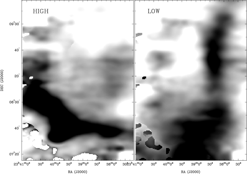
Figure 8: An integrated intensity image of two Gaussian components fitted to MS V velocity profiles. The grey-scale intensity range is 1 to 4 $\times 10^{19}$ cm^-2 for the higher velocity component, and 1.2 to 4 $\times 10^{19}$ cm^-2 for the lower velocity component.

5 Clump analyses

5.1 Clump identification

Figure 9: [f9.jpeg]Three fully mapped and well isolated clumps in the MS V region. For each clump, the left-hand side shows an HI intensity image overlaid with contours of the total column density, while the right-hand side shows a velocity profile at the clump’s center.

Figure 10: f10.jpeg] Four fully mapped and well isolated clumps in the MS VI region, from the top to the bottom. For each clump, the left-hand side shows an HI intensity image overlaid with contours of the total column density, while the right-hand side shows a velocity profile at the clump’s center.

Table 1: A summary of clump properties.

Clump ID	RA (J2000)	Dec (J2000)	LSR Velocity	Radius	FWHM	$T_{\rm peak}$
	(hh:mm:ss)	(dd:mm:ss)	(km s-1)	(arcmin)	(km s-1)	(K)
Small clumps
MS V:
1	23:40:23	07:58:45	$-354.5$	13	21.1	0.8
2	23:38:55	07:38:45	$-318.3$	18	18.6	0.7
3	23:38:07	07:36:45	$-344.2$	15	24.2	0.7
MS VI:
1	23:07:07	11:55:45	$-371.1$	13	20.7	1.0
2	23:07:55	13:03:45	$-363.3$	11	16.7	0.8
3	23:07:23	11:37:45	$-373.7$	12	16.3	0.8
4	23:06:19	12:23:45	$-391.8$	13	16.4	0.6
Large clumps
MS VH	23:40	08:10	$\sim-320$	64$\times$28	23.5	0.9
MS VL	23:39	08:19	$\sim-350$	54$\times$30	20.6	1.2
MS VI	23:07	12:22	$\sim-370$	65$\times$31	35.5	1.7

In order to study the properties of the MS clumps and the indirect clues they can provide about the properties of the Galactic Halo, we have attempted to identify individual clumps. We used two different approaches.

(i) To identify smaller clumps and sub-clumps within larger clumps, the three-dimensional clump-finding algorithm, ‘clfind’ coded in IDL (Williams et al., 1994) was applied to both data sets. A spatial binning by 4 pixels, and a velocity binning by 2 pixels was applied to reduce the computing time. ‘Clfind’ views data as a set of contour levels. It locates local maxima and defines clumps by tracing them by connecting pixels, at each contour level, that are within one resolution element of each other. The algorithm does not assume any particular geometry for the clumps. The most important input parameter for ‘clfind’ is the contour increment. This was set to twice the noise level, as recommended in Williams et al. (1994). All selected clumps were further vigorously inspected by eye by overlaying the ‘clfind’ output on the original data using the karma visualization package (Gooch, 1995). Only a few (seven) clumps that are isolated and fully inside the edges of our map were considered for further analysis. Those clumps, three in MS V and four in MS VI, are shown in Figs. 9 and 10. For each clump the central position, central velocity, clump size ($R_{\rm c}$) measured from the integrated intensity map, FWHM velocity line width ($\Delta v$), and peak brightness temperature were estimated and are listed in Table 1.

(ii) The clumps found by ‘clfind’ may or may not be distinct physical structures. On larger scales, all of MS VI and the ‘L’ and ‘H’ components of MS V could be considered as clumps themselves. The corresponding quantities for these three largest clumps are also listed in Table 1.

5.2 Observed and derived properties

Figure 11: Clump angular radius ($\theta_{\rm c}$) vs FWHM ($\Delta v$) for clumps in the MS VI region (filled circles), and in the MS V region (open circles). The whole MS VI region is shown as a star, and MS V ‘L’ and MS V ‘H’ components with downward and upward pointing triangles, respectively. Larson’s scaling law for the line width and cloud size, $\Delta v\propto\left[D\times\tan\left(\theta_{\rm c}\right)\right]^{0.5}$, is overlaid for the assumed distance $D=60$ kpc.

Fig. 11 shows the angular size and line width for all the clumps. A correlation between line width and cloud size has been found for interstellar clouds in a number of surveys (references in Vazquez-Semadeni et al. 1997). This is one of the famous Larson scaling laws: $\Delta v\propto R_{\rm c}^{\beta}$. For the case of self-gravitating molecular clouds $\beta=0.5$ (Myers & Goodman, 1988), a slightly flatter slope of 0.4 was found by Falgarone et al. (1992) in molecular clouds that are very little contaminated by star formation. We overlay the Larson relation in Fig. 11 for the assumed distance of 60 kpc. While all sub-clumps and one of the largest clumps (the whole of MS VI) appear to follow the correlation, two other large clumps have $\Delta v$ lower by about 10 km s^-1 than the predicted values.

We now derive several important clump properties. These properties depend on the assumed distance of the MS. Figs. 12 through 16 have double axes corresponding to the extreme distances of 60 and 20 kpc (see Section 2.2). For all these figures, the left-hand and bottom axes correspond to the far distance, and the right-hand and top axes correspond to the near distance.

The total HI mass is derived by integrating the brightness temperature over the entire line width. The HI mass is plotted as a function of cloud size in Fig. 12. For a given size our noise level sets a minimum detectable cloud mass. Using the narrowest measured clump line widths of $\sim$ 10 km s^-1  we get the threshold indicated by the dashed line on Fig. 12. Fig. 12 suggests that there may be many more structures like our clumps in MS V and MS VI which could be found by a more sensitive survey.

Assuming that clouds are spherically symmetric, using their HI mass and radius we can estimate an average HI volume density, $n_{\rm c}$. We find the values of $n_{\rm c}$ shown in Fig. 13, where the 3-$\sigma$ detection threshold is again shown by the dashed line. A typical value for the small clumps is 0.05 cm^-3 and for the large clumps 0.02 cm^-3, for the 60 kpc distance assumption. For the 20 kpc distance the volume density increases by a factor of three, as shown by the right-hand scale on Fig. 13.

Figure 12: The total HI mass ($M_{\rm HI}$) as a function of cloud size ($R_{\rm c}$) on a log–log scale. As previously, clumps in the MS VI region are shown as filled circles, and in the MS V region as open circles. The whole MS VI region is shown as a star, and MS V ‘L’ and MS V ‘H’ components with downward and upward pointing triangles, respectively. The dashed line shows our 3-$\sigma$ detection limit. The left-hand and bottom axes correspond to values derived assuming distance of 60 kpc, the right-hand and top axes correspond to the near distance of 20 kpc.

Figure 13: The average HI volume density ($n_{\rm c}$) as a function of cloud size ($R_{\rm c}$). The symbols and axes have the same meanings as in the preceding plots. The dashed line represents the 3-$\sigma$ detection limit.

6 Discussion

6.1 Cloud confinement

We now turn to cloud stability issues and the survival of the MS so far away from the MCs. There are several questions to ask about the HI structures which we find.

(1) Are the MS clumps gravitationally confined?
In order to be gravitationally confined, a clump’s escape velocity must be larger than $\Delta v$/2. This requires that the clump’s total mass is $M_{\rm grav}\geq R\Delta v^{2}/8G$. Fig. 14 compares the measured HI masses of our clumps with this hypothetical gravitational mass. For all our points $30<M_{\rm grav}/M_{\rm HI}<250$, if the distance of 60 kpc is assumed, and $120<M_{\rm grav}/M_{\rm HI}<750$, for the 20 kpc distance assumption. Thus gravitational confinement would require unreasonable amounts of dark matter.

Figure 14: The hypothetical gravitational mass ($M_{\rm grav}$) as a function of measured HI mass ($M_{\rm HI}$) on a log–log scale.

(2) Are the MS clumps unbound and freely expanding?
In the tidal model the MS age is 1.5 Gyr, while in the ram pressure model the age is 500 Myr. If the clouds are freely expanding their expansion time is given by: $t_{\rm exp}=2R/{\Delta v}$. These numbers are much less than the MS age. Fig. 15 plots the expansion age as a function of clump radius. The expansion age as a fraction of the MS age is indicated by the horizontal lines which apply to either model. This huge discrepancy between the expansion time and the age is the fundamental problem of the gas dynamics of the MS, as pointed out first by Mirabel et al. (1979). Barring the unreasonable dark matter halos required for gravitational confinement the simplest explanation is that the MS clouds are confined by a hot gaseous Galactic Halo.

Figure 15: Cloud expansion age ($t_{\rm exp}$) as a function of cloud size ($R_{\rm c}$). Dashed lines show $t_{\rm exp}$ as a fraction of the MS age.

6.2 Density of the Milky Way Halo

If the MS is confined by the Galactic Halo, then the external pressure, $P_{\rm h}=kn_{\rm h}T_{\rm h}$, must equal the clouds’ internal pressure $P_{\rm c}=kn_{\rm c}T_{\rm c}$: $P_{\rm c}\leq P_{\rm h}$. The relevant value of $T_{\rm c}$ is not the microscopic kinetic temperature but the total random motion of the atoms which we describe as a temperature defined by the line-width:

$$T_{\rm c}=\frac{\Delta v^{2}}{8\ln 2}\frac{k}{m_{\rm H}}=21.9~{}{\rm K}\times\left(\frac{\Delta v}{\rm km~{}s^{-1}}\right)^{2}.$$ (1)

Assuming a halo temperature of 10⁶ K and using $\Delta v$ for the clumps in Table 2 and the densities $n_{\rm c}$ illustrated on Fig. 13, we get Halo densities $n_{\rm h}$ shown in Fig. 16 as a function of distance from the Galactic Plane, $z$. Typical values for the near distance ($z\approx 15$ kpc) are $n_{\rm h}=10^{-3}$ cm^-3 and for the far distance ($z\approx 45$ kpc) are $n_{\rm h}=3\times 10^{-4}$ cm^-3. Note that these estimates are upper limits on the Halo density as magnetic, turbulent or ram pressure contributions were not included.

Figure 16: The logarithm of the Galactic Halo density ($n_{\rm h}$) as a function of distance from the Galactic Plane ($z$).

6.3 Expected Halo density

Current theories of galaxy formation predict the existence of a hot Galactic Halo containing the leftover gas which was unable to cool since the formation of the Galaxy. However, the density structure of the Halo is still very uncertain, especially at large distances from the Galactic Plane. Here we compare our results with several previous estimates, both observational and theoretical.

6.3.1 Observational constraints

The only direct observations of the hot Halo gas come from measurements of the soft X-ray background (Snowden et al., 1997). These X-ray maps reveal hot gas with a temperature $\sim 10^{6.6}$ K, a scale-height of 1.9 kpc and an electron density of $\sim$ 3.5$\times 10^{-3}$ cm^-3. Indirect observational constraints on the Halo density are more common. These are based on dispersion measure measurements of pulsars in globular clusters, or on the observational properties of HVCs, including the MS clouds.

Mirabel et al. (1979) estimate that $n_{\rm h}=7\times 10^{-4}$ – $7\times 10^{-5}$ cm^-3 for the distance range 10 – 100 kpc from HI observations of the MS and under similar confinement considerations as discussed in this paper. Similar values, $n_{\rm h}\geq 10^{-4}$ cm^-3, were suggested from H_α observations along the MS by Weiner & Williams (1996). Quilis & Moore (2001) applied the terminal velocity model by Benjamin & Danly (1997) for HVCs moving at $\sim 300$ km s^-1, at distances 10 – 100 kpc and with HI column density of $10^{20}$ cm^-2. This results in the requirement that $n_{\rm h}(10~{}{\rm kpc})<3\times 10^{-3}$ cm^-3 and $n_{\rm h}(100~{}{\rm kpc})<3\times 10^{-4}$ cm^-3, under the assumption that these are pure gas clouds. Our results agree well with the estimates from these three studies.

Another constraint for the Halo density at the distance of 130 kpc of $\sim 10^{-5}$ cm^-3 comes from HI observations of HVC 125$+$41$-$207 by Brüns et al. (2001). A significantly lower value for the upper limit on the Halo density, $n_{\rm h}(50~{}{\rm kpc})<10^{-5}$ cm^-3, was imposed by Murali (2000) by allowing the whole MS VI cloud to survive at the tip of the MS for about 500 Myr. We look more closely into this approach in Section 6.4.

6.3.2 Theoretical predictions

Benjamin & Danly (1997) considers a Galactic Halo consisting of three components: the warm ionized layer of HII parameterized by Reynolds (1993); the mean HI density distribution given by Dickey & Lockman (1990); and the hot Halo component with $T_{\rm h}=10^{6}$ K prescribed by Wolfire et al. (1995). While the first two components were parameterized observationally, the third component was constructed theoretically assuming an idealized isothermal halo in hydrostatic equilibrium, with the mid-plane density matching X-ray emission data by Garmire et al. (1992). The combination of all three components results in the analytic representation for $n_{\rm h}$ as a function of $z$ given by Benjamin & Danly (1997):

$$n_{\rm h}(z)=1.1\times 10^{-3}\left[1+\left(z^{2}_{\rm kpc}/19.6\right)\right]^{-1.35}{\rm cm}^{-3}.$$ (2)

At $z=15$ kpc the expected density is $n_{\rm h}=4\times 10^{-5}$ cm^-3, and at $z=45$ kpc $n_{\rm h}=2\times 10^{-6}$ cm^-3. These values are 25 – 150 times lower than those found in Section 6.2.

The ram-pressure model for the MS origin by Moore & Davis (1994) requires slightly higher values for the Halo density in order to match the kinematics of MS clouds:

$$n_{\rm h}=0.002/\left[1+\left(R/12~{}{\rm kpc}\right)\right]^{2}~{}{\rm cm^{-3}}.$$ (3)

Hence, at a distance of 20 kpc this yields a gaseous halo with $n_{\rm h}=3\times 10^{-4}$ cm^-3, while at a distance of 60 kpc $n_{\rm h}=6\times 10^{-5}$ cm^-3. Our estimates are much closer to the values predicted by this model but still several times higher.

6.4 Nature of Galactic infall

There are (at least) three different approaches present in the literature concerning the dynamics of clouds moving through an ambient medium. As understanding of the nature of this interaction can in turn provide clues about the properties of the Halo, here we discuss these approaches briefly.

(1) The mass loading approach
As the MS moves through the hot ambient Halo gas its clouds are subject to a drag force. Murali (2000) showed that this motion is actually dominated not by drag but by strong heating from accretion. If the Halo density is too high, heating due to accretion can cause cloud evaporation. This process is usually referred to as mass-loaded flow and it is common in comet interactions with the solar wind (Flammer, 1991). The Halo gas ionizes the cloud’s leading edges and picks up the ‘new material’ in a very asymmetric way that is constrained by the magnetic field: magnetic field lines slip past the cloud therefore allowing ablation of material only from the poles. Murali (2000) accounted for these effects and estimated that for the survival of the whole MS IV region for 500 Myr, at a distance of 50 kpc, $n_{\rm h}<10^{-5}$ cm^-3 is required. The key factor in this approach is the cooling resulting from a cloud’s mass-loss.

Following Murali’s calculations (their equation 1) for the MS V and MS VI clouds studied here, drag and accretion set a very low upper limit for the Halo gas density: $n_{\rm h}\sim 10^{-7}$ cm^-3 at $z=45$ kpc, and $n_{\rm h}\sim 10^{-6}$ cm^-3 at $z=15$ kpc, if mass-loss is not included. These values are significantly lower than theoretical predictions. Unless a significant cooling due to mass-loss is introduced, it is very hard for the hot Halo gas to exist in this model.

If the mass-loss rate, Ṁ$=2.5\times 10^{-2}$ M_⊙ yr^-1 (Murali 2000) is included, the requirements are comparable to our estimates: $n_{\rm h}\sim 3\times 10^{-4}$ cm^-3 at $z=45$ kpc and $n_{\rm h}\sim 3\times 10^{-3}$ cm^-3 at $z=15$ kpc. A slightly lower rate of Ṁ$=10^{-3}$ M_⊙ yr^-1 results in ten times lower Halo densities. However, the mass-loss rates of Ṁ$=10^{-3}$ or few$\times 10^{-2}$ M_⊙ yr^-1 throughout the whole cloud life-time are too high in comparison with the cloud HI masses discussed in Section 5.2. Such mass-loss rates would imply that cloud HI masses were 10 – 1000 times higher at the time of the MS formation. Smaller rates that are in agreement with the current HI masses are not sufficient to allow the existence of the Halo gas. Detailed simulations of the mass-loaded mechanism may help to constrain parameters such as mass-loss rate.

(2) Ballistic approach
Gregori et al. (1999) showed results of a 3-D study of a ballistic interaction of a moderately supersonic dense cloud with a warm magnetized medium. Since clouds are supersonic, their motion leads to the formation of a forward bow shock and a reverse crushing shock propagating through the cloud. As the cloud moves, its surface is subject to several instability mechanisms, the most disruptive of these being the Rayleigh-Taylor instability (R-T) that develops at the interface between two fluids when the lighter fluid accelerates the heavier one. These instabilities slowly disrupt the entire cloud and can dramatically change its morphology. In contrast to the mass-loaded flows, magnetic field lines here stay trapped, causing the development of strong magnetic pressure at the leading edge of the cloud.

The time-scale over which this dramatic change occurs is several times the so called ‘crushing time’, $\tau_{\rm CR}=2R_{\rm c}\chi^{1/2}/Mc_{\rm s}$, with $M$ being the Mach number, $\chi$ being the ratio of cloud to ambient density, and $c_{\rm s}$ being the sound speed. During a time shorter than $\tau_{\rm CR}$, the magnetic pressure is comparable to the ram pressure, while afterwards ram pressure dominates. For the MS clouds, $M\sim 2$, and assuming $\chi=100$ from Section 6.2, $\tau_{\rm CR}\sim 10$ – 30 Myr, depending on whether the near or far distance to the clouds is assumed. As ${\rm a~{}few}\times\tau_{\rm CR}$ is a significant fraction of the MS age this suggests that during a large fraction of a cloud’s life-time magnetic pressure may play a significant role. Inclusion of magnetic pressure in the calculations in Section 6.2 may somewhat reduce the required values for the Halo density.

(3) Hydrodynamical approach
Full hydrodynamical, 3-D simulations of HVCs moving through a diffuse hot gaseous component were performed recently by Quilis & Moore (2001). They investigated both pure gas clouds, being in pressure equilibrium with the external hot medium, and dark matter dominated clouds with an additional potential field that maintains their dynamical equilibrium. Particular cometary morphology, seen in the case of many HVCs as well as in many MS clouds, was reproduced for both cloud types but under the condition that the diffuse medium has density $n_{\rm h}>10^{-4}$ cm^-3.

6.5 Terminal velocity and neutral gas fraction

At the tip of the MS, clouds have had plenty of time to decelerate by a drag force (Murali 2000). The present velocity of the MS clouds is moderately supersonic (220 km s^-1 vs. sound speed c_s of $\sim 100$ km s^-1) suggesting that clouds are most likely now at the terminal velocity (Benjamin and Danly 1997). This means that clouds have stopped decelerating and that their boundary layers are subject to Kelvin-Helmholtz instabilities, while Rayleigh-Taylor instabilities are not important at this stage. Benjamin & Danly (1997) show that for a population of clouds with known distances, terminal velocities and column densities, it is possible to constrain the mean density of the gaseous halo and cloud neutral fraction $f_{\rm c}=N_{\rm HI}/(N_{\rm HI}+N_{\rm HII})$:

$$C_{\rm D}f_{\rm c}n_{\rm h}=\frac{2N_{\rm HI}g(z)}{v_{\rm T}^{2}},$$ (4)

here $C_{\rm D}$ is the drag coefficient, $g(z)$ is the gravitational acceleration, and $v_{\rm T}$ is the cloud’s terminal velocity. The mean column density for the MS V and MS VI clouds is $\langle\log N_{\rm HI}\rangle\approx 19$ cm^-3. Assuming that $v_{\rm T}=220$ km s^-1, the right-hand side of the equation does not depend on distance and has a mean value of $\langle C_{\rm D}f_{\rm c}\rho_{\rm h}\rangle\approx 6\times 10^{-4}$ cm^-3. If we assume $C_{\rm D}=1$ and apply Halo densities from Section 6.2, an estimate of the cloud’s neutral fraction can be obtained: at $z=15$ kpc $f_{\rm c}=0.6$, while at $z=45$ kpc $f_{\rm c}\geq 1$.

6.6 An alternative, gravitational confinement

An alternative explanation for cloud confinement is that they are gravitationally bound. This paradigm has been proposed for several compact HVCs (CHVCs) which are in some respects similar to MS V and MS VI clouds. An additional hint for this is provided by the peculiar velocity field seen in the MS VI region (Figs. 3 and 4), and discussed in Section 4.1, that may be interpreted as being due to differential rotation. In the case of three CHVCs, Braun & Burton (2000) found evidence for such orbital motion. In order to compare the MS VI cloud with these CHVCs we have attempted to model the velocity field north of Dec 12^∘30^′ using the tilted ring algorithm. The derived rotation curve has a quick and almost linear rise to $\sim$ 15 km s^-1, and then flattens out with large uncertainties.

This curve was used to obtain an estimate of the dynamical mass: $M_{\rm dyn}=1.5\times 10^{7}$ M_⊙ or $M_{\rm dyn}=5\times 10^{6}$ M_⊙, depending whether the far or near distance is assumed. This further implies dark-to-visible mass ratios of 50 to 180, respectively, after including a contribution by helium of 40% by mass to the observed HI mass. Therefore, if interpreted as a rotating HI cloud, this would require a very dark matter halo.

No model for the formation of the MS has ever predicted the existence of dark-matter dominated clouds in this gas filament. Even the parent galaxies, the MCs, are not rich in dark matter. It is therefore hard to believe that rotational support is realistic. This was the conclusion of Section 6.1. However the derived rotation curve is very similar to the rotation curves of CHVCs derived by Braun & Burton (2000). Dynamical masses of these CHVCs are about 10 times higher than the dynamical mass of the MS VI region, while the dark-to-visible mass ratio of the MS VI region is a few times higher than that for CHVCs. As the velocity field of MS VI is most likely the result of clump blending along the line-of-sight, it is interesting to note how well this effect can mimic differential rotation.

6.7 On the clump morphology

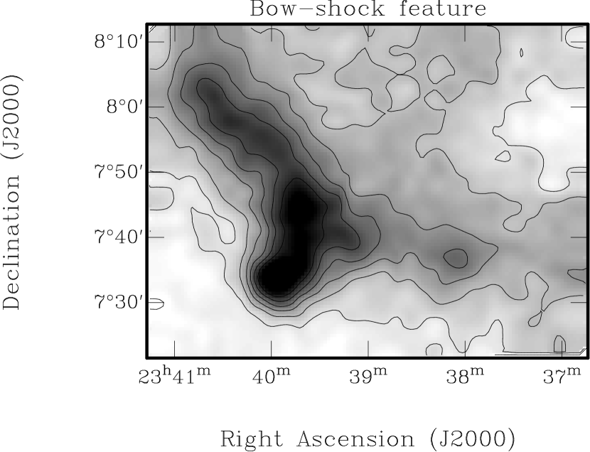
Figure 17: An HI intensity image of the bow-shock-like feature in the MS V region at the LSR velocity of $-351$ km s^-1.

Several clumps in the MS data cube show gradients in the brightness and velocity distribution, exhibiting a cometary or head-tail morphology. The best example is the south-eastern side of the MS V cloud at $-340$ to $-355$ km s^-1, see Fig. 17. This bow-shock-like feature may be a strong compression front, centered at RA 23^h 40^m, Dec 07^∘34^′ with two tails swept back on either side. This is strongly suggestive of a supersonic interaction between the HI cloud and an external, low density, ionized medium.

Similar cometary morphology is seen in many HVCs in surveys of Meyerdierks (1991) and Brüns et al. (2000). Putman (2000a) found many such clouds in the MS, which she speculated may be in the process of evaporation. The 3-D hydrodynamical simulations of an HVC moving through a diffuse hot medium by Quilis & Moore (2001) show a bow shock in front of the cloud, gas compression at the front edge of the cloud, and visible or invisible tails behind the cloud, depending on the density of the ambient medium. The double-tail morphology seen here is more similar to the simulations of the interaction between a disk-like structure with the surrounding medium by Quilis et al. (2000). These simulations were the first successful attempt to incorporate complex turbulent and viscous stripping at the interface of the cold and hot gaseous components. They predict a compression front and two tails folding on both sides. The similarity of the bow-shock-like feature with the simulations by Quilis et al. (2000) demonstrates the importance of turbulent and viscous mixing at the boundary layers when considering cloud – ambient medium interactions and should be fully explored in the future.

7 Conclusions

In this paper, we have presented new HI observations of two regions, MS V and MS VI, at the northern tip of the MS using the Arecibo telescope. The new data sets show the complex morphology of the MS with numerous inter-connected clumps. We have found double velocity structures in the MS V region. This region also contains an interesting bow-shock-like feature that is strongly suggestive of an interaction between the MS and an external medium. The MS VI data set shows a large velocity gradient, caused most likely by blending of small clumps along the line of sight. This region resembles the velocity field of a rotating disk, but we find that rotation is not a likely explanation.

Several MS clumps have been isolated to investigate their confinement mechanism. We show that unreasonably large amounts of dark matter are required in order for clumps to be gravitationally confined. Clumps do not seem to be in free expansion either. The easiest way to explain the clump properties is with external pressure confinement by the hot Galactic Halo. In this scenario we place an upper limit on the Halo density: $n_{\rm h}=10^{-3}$ cm^-3 at $z\approx 15$ kpc, and $n_{\rm h}=3\times 10^{-4}$ cm^-3 at $z\approx 45$ kpc. These values agree well with several previous indirect observations of the Halo, but are significantly higher than the values predicted theoretically for an isothermal hot Halo by Wolfire et al. (1995). Our results are closer to the expected Halo densities of the Moore & Davis model.

Although cloud evaporation is most likely an important process at the tip of the MS, the mass-loaded approach for cloud interaction with the ambient medium requires very high mass-loss rates to enable the existence of the hot Halo gas. The ballistic consideration of clouds in the Halo suggests that during a large fraction of the cloud lifetime magnetic pressure may have a significant role in cloud evolution. Inclusion of magnetic pressure would reduce somewhat the required values for the Halo density.

Hydrodynamical modeling of cloud interaction with the ambient medium also requires high Halo densities to reproduce cometary features commonly seen in HI observations of HVCs. If we assume that MS clouds are at their terminal velocity, the cloud’s neutral fraction can be estimated at $z=15$ kpc $f_{\rm c}=0.6$, while at $z=45$ kpc $f_{\rm c}\geq 1$.

References

- Benjamin & Danly (1997) Benjamin, R. A. & Danly, L. 1997, ApJ, 481, 764
- Bland-Hawthorn & Maloney (1999) Bland-Hawthorn, J. & Maloney, P. R. 1999, ApJ, 510, L33
- Bland-Hawthorn & Maloney (2002) —. 2002, in Extragalactic Gas at Low Redshift, ed. J. M. . J. Stocke, ASP Conference Series (San Francisco: Astronomical Society of the Pacific), in press
- Bland-Hawthorn & Putman (2001) Bland-Hawthorn, J. & Putman, M. E. 2001, in ASP Conf. Ser. 240: Gas and Galaxy Evolution, 369
- Braun & Burton (2000) Braun, R. & Burton, W. B. 2000, A&A, 354, 853
- Brüns et al. (2001) Brüns, C., Kerp, J., & Pagels, A. 2001, A&A, 370, L26
- Brüns et al. (2000) Brüns, C., Kerp, J., & Staveley-Smith, L. 2000, in ASP Conf. Ser. 218: Mapping the Hidden Universe: The Universe behind the Mily Way - The Universe in HI, 349
- Cohen & Davies (1975) Cohen, R. J. & Davies, R. D. 1975, MNRAS, 170, 23P
- Dickey & Lockman (1990) Dickey, J. M. & Lockman, F. J. 1990, A&AR, 28, 215
- Dickey et al. (2001) Dickey, J. M., McClure-Griffiths, N. M., Stanimirović, S., Gaensler, B. M., & Green, A. J. 2001, ApJ, 561, 264
- Dieter (1965) Dieter, N. H. 1965, AJ, 70, 552
- Elmegreen et al. (2001) Elmegreen, B. G., Kim, S., & Staveley-Smith, L. 2001, ApJ, 548, 749
- Erkes et al. (1980) Erkes, J. W., Philip, A. G. D., & Turner, K. C. 1980, ApJ, 238, 546
- Falgarone et al. (1992) Falgarone, E., Puget, J.-L., & Perault, M. 1992, A&A, 257, 715
- Fiedler et al. (1994) Fiedler, R., Dennison, B., Johnston, K. J., Waltman, E. B., & Simon, R. S. 1994, ApJ, 430, 581
- Flammer (1991) Flammer, K. R. 1991, in ASSL Vol. 167: IAU Colloq. 116: Comets in the post-Halley era, 1125–1144
- Gardiner (1999) Gardiner, L. T. 1999, in IAU Symp. 190: New Views of the Magellanic Clouds, Vol. 190, 480
- Gardiner & Noguchi (1996) Gardiner, L. T. & Noguchi, M. 1996, MNRAS, 278, 191
- Gardiner et al. (1994) Gardiner, L. T., Sawa, T., & Fujimoto, M. 1994, MNRAS, 266, 567
- Garmire et al. (1992) Garmire, G. P., Nousek, J. A., Apparao, K. M. V., Burrows, D. N., Fink, R. L., & Kraft, R. P. 1992, ApJ, 399, 694
- Gooch (1995) Gooch, R. 1995, in ASP Conference Series, Vol. 77, Astronomical Data Analysis and Software Systems V, ed. R. A. Shaw, H. E. Payne, & J. J. E. Hayes (San Francisco: Astronomical Society of the Pacific), 144
- Green (1993) Green, D. A. 1993, MNRAS, 262, 327
- Gregori et al. (1999) Gregori, G., Miniati, F., Ryu, D., & Jones, T. W. 1999, ApJ, 527, L113
- Heiles et al. (2001) Heiles, C., Perillat, P., Nolan, M., Lorimer, D., Bhat, R., Ghosh, T., Howell, E., Lewis, M., O’Neil, K., Salter, C., & Stanimirovic, S. 2001, PASP, 113, 1247
- Heller & Rohlfs (1994) Heller, P. & Rohlfs, K. 1994, A&A, 291, 743
- Konz et al. (2001) Konz, C., Lesch, H., Birk, G. T., & Wiechen, H. 2001, ApJ, 548, 249
- Lazarian & Pogosyan (2000) Lazarian, A. & Pogosyan, D. 2000, ApJ, 537, 720L
- Lin & Lynden-Bell (1982) Lin, D. N. C. & Lynden-Bell, D. 1982, MNRAS, 198, 707
- Maddison et al. (2002) Maddison, S. T., Kawata, D., & Gibson, B. K. 2002, in The Evolution of Galaxies II: Basic Building Blocks, ed. M. S. et al. (Kluwer), in press
- Mathewson et al. (1974) Mathewson, D. S., Cleary, M. N., & Murray, J. D. 1974, ApJ, 190, 291
- Mathewson & Ford (1984) Mathewson, D. S. & Ford, V. L. 1984, in Structure and Evolution of the Magellanic Clouds, ed. S. van der Bergh & K. de Boer, I.A.U. Symposium No. 108 (Reidel, Dordrecht), 125
- Mathewson et al. (1977) Mathewson, D. S., Schwarz, M. P., & Murray, J. D. 1977, ApJ, 217, L5
- Mathewson et al. (1987) Mathewson, D. S., Wayte, S. R., Ford, V. L., & Ruan, K. 1987, Proceedings of the Astronomical Society of Australia, 7, 19
- McGee & Newton (1986) McGee, R. X. & Newton, L. M. 1986, Proceedings of the Astronomical Society of Australia, 6, 471
- Meyerdierks (1991) Meyerdierks, H. 1991, A&A, 251, 269
- Mirabel (1981) Mirabel, I. F. 1981, ApJ, 250, 528
- Mirabel et al. (1979) Mirabel, I. F., Cohen, R. J., & Davies, R. D. 1979, MNRAS, 186, 433
- Moore & Davis (1994) Moore, B. & Davis, M. 1994, MNRAS, 270, 209
- Murai & Fujimoto (1980) Murai, T. & Fujimoto, M. 1980, PASJ, 32, 581
- Murali (2000) Murali, C. 2000, ApJ, 529, L81
- Myers & Goodman (1988) Myers, P. C. & Goodman, A. A. 1988, ApJ, 329, 392
- Putman (2000a) Putman, M. E. 2000a, Ph.D thesis (Mount Stromlo Observatory, Australia: The Australian National University)
- Putman (2000b) —. 2000b, Publications of the Astronomical Society of Australia, 17, 1
- Putman & Gibson (1999) Putman, M. E. & Gibson, B. K. 1999, Publications of the Astronomical Society of Australia, 16, 70
- Putman et al. (1998) Putman, M. E., Gibson, B. K., Staveley-Smith, L., Banks, G., Barnes, D. G., Bhatal, R., Disney, M. J., Ekers, R. D., Freeman, K. C., Haynes, R. F., Henning, P., Jerjen, H., Kilnborn, V., Koribalski, B., Knezek, P., Malin, D. F., Mould, J. R., Osterloo, T., Price, R. M., Ryder, S. D., Sadler, E. M., Stewart, I., Stootman, F., Vaile, R. A., Webster, R. L., & Wright, A. E. 1998, Nat, 394, 752
- Putman et al. (2002) Putman, M. E., Staveley-Smith, L., Freeman, K. C., Gibson, B. K., & Barnes, D. G. 2002, ApJ, submitted
- Quilis & Moore (2001) Quilis, V. & Moore, B. 2001, ApJ, 555, L95
- Quilis et al. (2000) Quilis, V., Moore, B., & Bower, R. 2000, Science, 288, 1617
- Reynolds (1993) Reynolds, R. J. 1993, in AIP Conf. Proc. 278: Back to the Galaxy, 156
- Snowden et al. (1997) Snowden, S. L., Egger, R., Freyberg, M. J., McCammon, D., Plucinsky, P. P., Sanders, W. T., Schmitt, J. H. M. M., Truemper, J., & Voges, W. 1997, ApJ, 485, 125
- Sofue (1994) Sofue, Y. 1994, PASJ, 46, 431
- Sramek & Schwab (1989) Sramek, R. A. & Schwab, F. R. 1989, in ASP Conference Series, Vol. 6, Synthesis imaging in radio astronomy, ed. R. Perley, F. Schwab, & A. Bridle (San Francisco: Astronomical Society of the Pacific), 117
- Stanimirovic et al. (2002) Stanimirovic, S., Dickey, J. M., & Brooks, A. M. 2002, in Gaseous Matter in Galaxies and Intergalactic Space, XVIIth IAP Colloquium, eds. R. Ferlet, M. Lemoine, J.-M. Desert, & B. Raban, 199
- Stanimirovic et al. (1999) Stanimirovic, S., Staveley-Smith, L., Dickey, J. M., Sault, R. J., & Snowden, S. L. 1999, MNRAS, 302, 417
- Staveley-Smith et al. (1997) Staveley-Smith, L., Sault, R. J., Hatzidimitriou, D., Kesteven, M. J., & McConnell, D. 1997, MNRAS, 289, 225
- Vazquez-Semadeni et al. (1997) Vazquez-Semadeni, E., Ballesteros-Paredes, J., & Rodriguez, L. F. 1997, ApJ, 474, 292
- Wakker (2001) Wakker, B. P. 2001, ApJS, 136, 463
- Wannier & Wrixon (1972) Wannier, P. & Wrixon, G. T. 1972, ApJ, 173, L119
- Wayte (1989) Wayte, S. R. 1989, Proceedings of the Astronomical Society of Australia, 8, 195
- Weiner et al. (2002) Weiner, B. J., Vogel, S. N., & Williams, T. B. 2002, in ASP Conference Series, Vol. 666, Extragalactic Gas at Low Redshift, ed. J. Mulchaey & J. Stocke (San Francisco: Astronomical Society of the Pacific), in press
- Weiner & Williams (1996) Weiner, B. J. & Williams, T. B. 1996, AJ, 111, 1156
- Westpfahl et al. (1999) Westpfahl, D. J., Coleman, P. H., Alexander, J., & Tongue, T. 1999, ApJ, 117, 868
- Williams et al. (1994) Williams, J. P., de Geus, E. J., & Blitz, L. 1994, ApJ, 428, 693
- Wolfire et al. (1995) Wolfire, M. G., McKee, C. F., Hollenbach, D., & Tielens, A. G. G. M. 1995, ApJ, 453, 673
- Yoshizawa & Noguchi (1999) Yoshizawa, A. M. & Noguchi, M. 1999, in IAU Symp. 186: Galaxy Interactions at Low and High Redshift, Vol. 186, 60