Short-Spacings Correction from the Single-Dish Perspective

Abstract

While, in general, interferometers provide high spatial resolution for imaging small-scale structure (corresponding to high spatial frequencies in the Fourier plane), single-dishes can be used to image the largest spatial scales (corresponding to the lowest spatial frequencies), including the total power (corresponding to zero spatial frequency). For many astrophysical studies, it is essential to bring ‘both worlds’ together by combining information over a wide range of spatial frequencies. This article demonstrates the effects of missing short-spacings, and discusses two main issues: (a) how to provide missing short-spacings to interferometric data, and (b) how to combine short-spacing single-dish data with those from an interferometer.

National Astronomy and Ionosphere Center, Arecibo Observatory, HC 3 Box 53995, Arecibo, Puerto Rico 00612, USA

1. Introduction

All radio telescopes can be classified as either filled or unfilled-aperture antennas. The simplest filled-aperture antennas are single-dish telescopes. The desired astronomical object to be observed and the particular scientific goals determine which type of radio telescope to use. In general, single-dishes are considered as tools for low spatial resolution observations, while interferometers are used for high resolution observations. While compact objects are more suited for interferometric observations, extended objects are commonly observed with single-dishes as interferometers cannot faithfully recover information on the largest spatial scales.

However, in many scientific cases it is essential to obtain high spatial resolution observations of large objects, and to accurately represent emission present over a wide range of spatial scales. A simple recipe you may follow in such cases is:

• observe (mosaic) your object with an interferometer,

• observe your object with a single-dish,

• cross-calibrate the two data sets, and then

• combine the single-dish and interferometer data.

This combination of single-dish and interferometer data, when observing extended objects, is referred to as the short-spacings correction.

This ‘simple’ recipe may be considered as an artistic touch to the interferometric images as it makes them look much nicer but still preserves their high spatial resolution. This results from: (a) inclusion of more resolution elements, those seen by a single-dish; and (b) reconstruction of image artifacts. At the same time, these images contain information about the total power, and can be used to measure accurate flux densities, column densities, masses, etc. From a pure historical perspective, the short-spacings correction bridges the gap between the two classes of radio telescopes, essentially obtaining the best of ‘both worlds’, that is the high spatial resolution information provided by interferometers, and the low spatial resolution, including the total power, information provided by single-dishes.

This article will explain what the short-spacing problem is, how it is manifested, and how we can, both theoretically and practically, solve this problem. Section 2 depicts very briefly the fundamentals of interferometry, defines the spatial frequency domain, and draws an analogy between a single dish and an interferometer. The effects of missing short spacings are demonstrated in Section 3, as well as prospects for solving the problem. Section 4 considers the cross-calibration of interferometer and single dish data which is a precursor to any combination method. Methods for data combination are discussed in Section 5 and Section 6, and compared in Section 7.

2. A Very Brief Introduction to Interferometry

Figure 1.: [fig1.jpeg]A schematic diagram of the spatial frequency and image coordinate systems. The spatial frequency domain, $(u,v,w)$, is used to express the interferometer baseline, and the image domain, $(l,m,n)$, is used to express the source brightness distribution. The direction to the center of the field of view is given by ${\bf s}_{0}$, and to any given position by ${\bf s}$. Hence, ${\bf s}={\bf s_{0}}+\mbox{\boldmath{$\sigma$}}$. (From Thompson 1994.)

A very brief review of the basics of interferometry is necessary right at the beginning of this article, in order to define and explain some terms that will be used further on. However, we do not want to go deeply into interferometry, as there is a vast literature available on this topic, starting with “Interferometry and Synthesis in Radio Astronomy” (Thompson, Moran, & Swenson 1986) and “Synthesis Imaging in Radio Astronomy” (Taylor, Carilli, & Perley 1999).

The fundamental idea behind interferometry is that a Fourier transform relation exists between the sky radio brightness distribution $I$ and the response of a radio interferometer. If the distance between two antennas (the baseline) is ${\bf d}$, then the so-called visibility function, $V({\bf d})$, is given by:

$$V({\bf d})=\int_{\rm source}A(\mbox{\boldmath{$\sigma$}})I(\mbox{\boldmath{$\sigma$}})\exp\left[-2\pi i~{}{\bf d}\cdot\mbox{\boldmath{$\sigma$}}/\lambda\right]d\Omega\;.$$ (1)

Here, $A(\mbox{\boldmath{$\sigma$}})$ is an antenna reception pattern, or primary beam, and $\sigma$ is the vector difference between a given celestial position and the central position of the field of view. The aperture synthesis technique is a method of solving Equation 1 for $I(\mbox{\boldmath{$\sigma$}})$ by measuring $V$ at suitable values of ${\bf d}$.

To simplify Equation 1, a more convenient, right-hand rectilinear, coordinate system is introduced in Fugure 1. Coordinates of vector ${\bf d}$ in this system are $(u,v,w)$, where the direction to the source center ${\bf s}_{0}$ defines the $w$ direction, and $u$ and $v$ are baseline projections onto the plane perpendicular to the ${\bf s}_{0}$ direction, towards the East and the North, respectively. A synthesized image in the $l-m$ plane represents a projection of the celestial sphere onto a tangential plane at the source center. In certain conditions, that is in the case of an Earth tracking, East-West interferometer array, with the $w$-axis lying in the direction of the celestial pole, further simplifications of Equation 1 are possible:

$$V(u,v)=\int\int A(l,m)I(l,m)\exp[-2\pi i(ul+vm)]\frac{dldm}{\sqrt{1-l^{2}-m^{2}}}\;.$$ (2)

Therefore, the visibility function $V(u,v)$ can be expressed as the Fourier transform of a modified brightness distribution $A(l,m)I(l,m)$. Coordinates $u$ and $v$ ($w=0$) are measured in units of wavelength and the $u-v$ plane is called the spatial frequency domain. These are effectively projections of a terrestrial baseline onto a plane perpendicular to the source direction. The $l-m$ plane is referred to as the image domain. To obtain $I(l,m)$, from Equation 2, an inverse Fourier transform of $V(u,v)$ is required, meaning that a complete sampling of the spatial frequency domain is essential. In practice however, a bit more than a simple inversion is needed as only limited sampling of the $u-v$ plane is available.

2.1. How do we ‘fill in’ the $u-v$ plane?

Figure 2.: [fig2.jpeg]The $u-v$ coverage for an 8 hr tracking observation with the VLA, for an object at declination of 30^∘ (from Burke & Graham-Smith 1997).

For a given configuration of antennas any interferometer array has a limited range of baselines, lying between a minimum, $d_{\rm min}$, and maximum, $d_{\rm max}$, baselines. As an example, 5 antennas of the Australia Telescope Compact Array (ATCA) form 10 baselines, with $d_{\rm min}=31$ m and $d_{\rm max}=459$ m for a particularly compact configuration. The final resolution ($\theta_{\rm int}$) is inversely related to the maximum baseline by $\theta_{\rm int}\approx\lambda/d_{\rm max}$. In the case of an Earth tracking interferometer, as the Earth rotates the baseline projections on the $u-v$ plane trace a series of ellipses. The parameters of each ellipse depend upon the declination of the source, the length and orientation of the baseline, and the latitude of the center of the baseline (Thompson et al. 1986). The ellipses are concentric for a linear array (e.g. ATCA). For a 2-dimensional array (e.g. the Very Large Array, VLA), the ellipses are not concentric and so can intersect.

As each baseline traces a different ellipse, the ensemble of ellipses indicates the spatial frequencies that can be measured by the array (see Thompson et al. 1986). At each sampling interval, the correlator measures the visibility function for each baseline, thus resulting in a number of samples being measured over elliptical tracks in the $u-v$ plane. Hence, the resultant interferometer $u-v$ coverage will always be, more or less, incomplete, having a hole in the center of the $u-v$ plane whose diameter corresponds to the minimum baseline, gaps between measured elliptical tracks, and gaps between each adjacent samples on each elliptical track. The ensemble of ellipses (loci) is known as the transfer or sampling function, $b_{\rm int}(u,v)$. An example of the sampling function obtained with the VLA is shown in Fugure 2.

Hence, if $V(u,v)$ is a true (ideal) visibility function, the measured (observed) visibilities ($V_{\rm int}^{\prime}$) can be expressed as:

$$V^{\prime}_{\rm int}(u,v)=V(u,v)b_{\rm int}(u,v)\;.$$ (3)

$b_{\rm int}$ is usually representable by a set of $\delta$-functions, between the lowest and the highest spatial frequency sampled by the interferometer (corresponding to the shortest and the longest baselines, respectively). The Fourier transform of Equation 3 gives the observed sky brightness distribution $I_{\rm int}^{\rm D}$ (so called ‘dirty’ image):

$$I_{\rm int}^{\rm D}(l,m)=I(l,m)*B_{\rm int}(l^{\prime},m^{\prime})\;,$$ (4)

where $B_{\rm int}$ is the synthesized or ‘dirty’ beam, which is the point source response of the interferometer. As usually, asterisks ($*$) are used to denote convolution. When imaging, incomplete $u-v$ coverage leads to severe artifacts, such as negative ‘bowls’ around emission regions and negative and positive sidelobes (Cornwell, Braun, & Briggs 1999). We return to this in Section 3. The determination of $I$ from $I_{\rm int}^{\rm D}$ in the deconvolution process, requires beforehand interpolation and extrapolation of $V_{\rm int}^{\prime}$ for missing data due to the discontinuous nature of $b_{\rm int}$ (Cornwell & Braun 1989). This process works well when a compact configuration of antennas is used and when the source is small enough, with angular size $\theta\leq 2\lambda/d_{\rm min}$ (Bajaja & van Albada 1979).

For imaging larger objects, with angular size $\theta>\lambda/d_{\rm min}$, a significant improvement in filling in the $u-v$ coverage can be achieved by using the ‘mosaicing technique’, where observations of many pointing centers are obtained and ‘pasted’ together (see Holdaway 1999). Mosaicing effectively reduces the shortest projected baseline to $d_{\rm min}-D/2$, where $D$ is the diameter of an individual antenna. Nevertheless, the center of the $u-v$ plane still suffers if significant large scale structure is present. This lack of information for very low spatial frequencies (around the center of the $u-v$ coverage) in an interferometric observation is usually referred to as the ‘short-spacings problem’.

2.2. A single-dish as an interferometer?

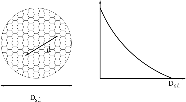
Figure 3.: A schematic representation of a single dish as an interferometer with a large number of elements and a monotonically decreasing distribution of baselines ($d$) from zero to $D_{\rm sd}$.

Extended objects with angular size $\theta>\lambda/d_{\rm min}$ can be observed with a single-dish. Let us now think of a single-dish in a slightly unusual way, imagining filled apertures consisting of a large number of small panels packed closely together. Then all these panels can act as interferometer elements with their signals being combined together at the focus, making a so called phased or adding array (see contribution by D. Emerson in this volume). The distance between each two panels corresponds to a baseline, as shown in Fugure 3. The baseline distribution then monotonically decrease from zero at the center up to the maximum baseline, determined by the single-dish diameter $D_{\rm sd}$. This is also shown in Fugure 3.

One observation with a single-dish provides a total flux density measurement, corresponding to the zero spacing, $(u,v)=(0,0)$. However, if a single-dish scans across an extended celestial object, it measures not only a single spatial frequency, but a whole range of continuous spatial frequencies all the way up to a maximum of $D_{\rm sd}$ (Ekers & Rots 1979). Hence, a single-dish behaves as an interferometer with an almost infinite number of antennas, and therefore has a continuous range of baselines, from zero up to $D_{\rm sd}$. The nice thing about this representation is that we can now use the same mathematical notation to describe both single-dishes and interferometers.

The observed sky brightness distribution $I_{\rm sd}^{\rm D}$ in the case of single-dish observations is then given by:

$$I_{\rm sd}^{\rm D}(l,m)=I(l,m)*B_{\rm sd}(l^{\prime},m^{\prime}),$$ (5)

with $B_{\rm sd}$ being the single-dish beam pattern. The Fourier transform of Equation 5 gives the observed single-dish ‘visibilities’, $V_{\rm sd}^{\prime}$:

$$V_{\rm sd}^{\prime}(u,v)=V(u,v)\times b_{\rm sd}(u,v)$$ (6)

where $b_{\rm sd}$ is the Fourier transform of the single-dish beam pattern which, unlike $b_{\rm int}$, is a continuous function between zero and the highest spatial frequency sampled by the single-dish. Determination of $I$ from $I_{\rm sd}^{\rm D}$ requires deconvolution, but no interpolation of $V_{\rm sd}^{\prime}$ is needed since this is a continuous function.

Figure 4.: [fig4.jpeg]An HI image of the SMC from Stanimirovic et al. (1999) is shown on the left. The observations were obtained as a mosaic of 320 different pointing centers with the ATCA. Positive intensity values are shown in black, while white represents negative pixel values. RA cuts through the image, at Dec $-72^{\circ}$ $02^{\prime}$ $54^{\prime\prime}$ and Dec $-73^{\circ}$ $05^{\prime}$, are shown on the right.

3. How is the Short-spacings Problem Manifested?

As shown in Equation 4, the sky brightness distribution can be reconstructed, in the case of interferometric observations, by deconvolving the ‘dirty’ image with the synthesized beam. As an example, Fugure 4 shows the result of the HI ‘mosaic’ observations of the Small Magellanic Cloud (SMC) with the ATCA. More information about these observations and data reduction is available in Stanimirovic et al. (1999). The two adjacent panels on the right side show right ascension (RA) cuts through the image. Negative bowls (shown in white on the image) are seen around emission peaks (shown in black), as well as in RA cuts. These are typical interferometric artifacts resulting from an incomplete $u-v$ coverage.

A simple graphical explanation of why this happens, borrowed from Braun & Walterbos (1985), is shown in Fugure 5 for the case of a point source. The solid vertical line in Fugure 5 distinguishes the spatial frequency (a) from the image domain (b). The distribution of measured spatial frequencies, or what we have already defined as a transfer (or sampling) function, $b_{\rm int}$, is given on the left side, while its Fourier transform, that is the synthesized beam, $B_{\rm int}$, is shown in the right. An exclusion of the central values from the spatial frequency domain, is equivalent to a subtraction of a broad pedestal in the image domain, resulting in the presence of a deep negative ‘bowl’ around the observed object, as seen in Fugure 4.

This demonstrates simply how severe the effects of missing short-spacings can be. The larger the object is relative to the reciprocal of the shortest measured baseline one tries to image, the more prominent the short-spacing problem becomes.

Figure 5.: [fig5.jpeg] A 1-dimensional cut through $(u,v)=(0,0)$ of the spatial frequency domain, (a), and its corresponding manifestation in the image domain, (b). An exclusion of the central values from the spatial frequency domain is equivalent to a subtraction of a broad pedestal in the image domain, resulting in the presence of a deep negative ‘bowl’ around the observed object. (From Braun & Walterbos 1985.)

3.1. How can we solve the short-spacings problem?

There are two main questions concerning the short-spacings problem:

1. how to provide (observe) missing short spacings to interferometric data;

2. how to combine short-spacing data with those from an interferometer.

In answering the first question, all solutions can be grouped into two array schemes: homogeneous, having all antennas of the same size, and heterogeneous, based on observations obtained with different-sized antennas. There are many possibilities concerning the heterogeneous arrays, such as using smaller arrays and even a hierarchy of smaller arrays. The simplest option, though, is a single-dish telescope with a diameter ($D_{\rm sd}$) larger than the interferometer’s minimum baseline.

We briefly touch here on some pros and cons for both array schemes. One of the difficulties in providing short-spacings with a single-dish is that it is hard to provide a large single-dish which would have the sensitivity equivalent to that of an interferometer (Holdaway 1999). Also, single-dish observations are complex (they require a lot of separate pointing centers to cover a large object) and very sensitive to systematic errors. Using theoretical analysis, numerical simulations and observational tests, Cornwell, Holdaway, & Uson (1993) show that a homogeneous array in which the short-spacings are obtained from single antennas of the array, allows high quality imaging. They find that a key advantage over the large single-dish scheme is pure simplicity, which is an important factor for the complex interferometric systems. As both interferometric and total power data are obtained with the same array elements, no cross-calibration is required in this case. Note that in this case total-power and interferometric observations have to be synchronized which is not a simple task because of different observing techniques involved (e.g. the single-dish observations require frequency or position switching modes!). This turns out to be an especially difficult task for the continuum observations.

However, to fully fill in the central gap in an interferometer $u-v$ coverage and preserve sensitivity at the same time, the heterogeneous array scheme appears more advantageous. This has been recently recognized in the planning of the future Atacama Large Millimeter/Submillimeter Array (ALMA). Imaging simulations have shown that antenna pointing errors of only a few percent of the primary beam width produce large errors in the visibilities in the central $u-v$ plane, causing a large degradation of image quality (see Morita 2001). To compensate for this problem, an additional, smaller array of 6 – 8 m dishes, the so called ALMA Compact Array (ACA), has been proposed to provide short baselines.

In answering the second question, methods for the combination of interferometer and single-dish data can be grouped into two classes: data combination in the spatial frequency domain (Bajaja & van Albada 1979; Vogel et al. 1984; Roger et al. 1984; Wilner & Welch 1994; Zhou, Evans, & Wang 1996), and data combination in the image domain (Ye & Turtle 1991; Stewart et al. 1993; Schwarz & Wakker 1991; Holdaway 1999). Each approach can be realized through a number of different methods. Both approaches are very common and are becoming a standard data processing step.

As the most common scheme of a heterogeneous array involves use of a large single-dish telescope, we proceed to consider this particular case further.

4. Cross-calibration of Interferometer and Single-dish Data

Before adding short-spacing data, it is necessary to be sure that both the interferometer and single-dish data sets have identical flux density scales. As calibration is never perfect, the calibration differences between the two sets of observations can be significant in some cases (e.g. observations spread over a long period of time, different data quality, use of different flux density scales for calibration, quality of calibrators, etc.). This results in a small but appreciable difference in the measured flux densities.

We define the calibration scaling factor, $f$, as the ratio of the flux densities of an unresolved source in the single-dish and interferometer maps:

$$f=\frac{S_{\rm int}}{S_{\rm sd}}\;.$$ (7)

In the case of perfect calibration, $f=1$. However, $f\neq 1$ otherwise, and needs to be determined very accurately. Unfortunately, it is hard to find suitable compact sources to directly determine $f$. Hence, the best way to estimate $f$ is to compare the surface brightness of the observed object in the overlap region of the $u-v$ plane, see Fugure 6. This region should correspond to angular sizes to which both telescopes are sensitive. For a source of brightness, $I$, both the interferometer and single dish should measure within this region the same, $I_{\rm sd}=I_{\rm int}$, and calibration errors will appear as:

$$f=\frac{I_{\rm int}}{I_{\rm sd}}\;.$$ (8)

For an extended source $I_{\rm int}$ and $I_{\rm sd}$ are often, for convenience, expressed in units of Jy beam^-1 not Jy sr^-1, and so will be different numbers because of the different beams considered (with beam areas $\Omega_{\rm int}$ and $\Omega_{\rm sd}$, respectively). For this purpose, an estimate of the resolution difference between the two data sets ($\alpha=\Omega_{\rm int}/\Omega_{\rm sd}$) is also needed.

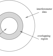
Figure 6.: A schematic diagram of the spatial frequency domain of an observation in a heterogeneous scheme when using a single-dish for providing short-spacings: the inner spatial frequencies are sampled by the single-dish only, the outer ones are sampled only by the interferometer, while the overlapping region contains spacings to which both the single-dish and interferometer are sensitive.

To determine $f$ the following steps are required:

1. scale the single-dish data by $\alpha$ to account for the difference in brightness caused only by different resolutions,

2. Fourier transform the interferometer and scaled single-dish images,

3. deconvolve the single-dish data (by dividing them by the Fourier transform of the single-dish beam), and

4. compare ‘visibilities’ in the overlapping region of spatial frequencies.

Several important issues should be considered here:

• When Fourier transforming in Step 2 watch for edge-effects! To avoid nasty edge-effects in some cases apodizing of both interferometer and single-dish images may be required in order to make the image intensities smoothly decrease to zero near the edges.

• Step 3 requires a very good knowledge of the single-dish beam! To make things even harder, the FWHM of the single-dish beam and the calibration scaling factor are highly coupled (Sault & Killeen 1998). Therefore, an error in the single-dish beam model has the same effect in the overlapping region as an error in the flux density scale. If the single-dish beam is poorly known, $f$ will be a quadratic function of distance in the Fourier plane, in the first approximation (see Stanimirovic 1999).

• A sufficient overlap in spatial frequency is required for Step 4. Assuming a Gaussian-tapered illumination pattern for a single-dish, and considering a cut-off level of 0.2 for reliable data, we can estimate the minimum diameter, $D$, of a single-dish necessary to provide all spacings shorter than $d_{\rm min}$ for a given interferometer:

  $$D>1.5\times d_{\rm min}\;.$$ (9)

  In order to have a reasonable overlap of spatial frequencies so that $f$ can be derived, a slightly larger single-dish is required with $D>2\times d_{\rm min}$. For example, for the ATCA shortest baseline of 31 m, the single-dish providing short spacings should have diameter of $D\geq 62$ m. Therefore, the 64 m Parkes telescope can do a really great job. Also, while the 100-m Green Bank Telescope will be able to provide short-spacing data for the VLA C and D arrays (with $d_{\rm min}=35$ m), only Arecibo could do so for the VLA B array (with $d_{\rm min}=210$ m).

5. Data Combination in the Spatial Frequency Domain

5.1. Theoretically…

As shown by Bajaja & van Albada (1979), the true missing short-spacing visibilities can be provided from the function $V(u,v)$ in Equation 6, if the single-dish is large enough to cover the whole central gap in the interferometer $u-v$ coverage. The deconvolution of the single-dish data gives the true single-dish visibilities, where $b_{\rm sd}(u,v)\neq 0$, by:

$$V(u,v)=\frac{V_{\rm sd}^{\prime}(u,v)}{b_{\rm sd}(u,v)}\;.$$ (10)

Function $V(u,v)$ can be then substituted in Equation 3, after rescaling by $f$, everywhere in the $u-v$ plane where Equation 10 holds. This would provide the resultant $u-v$ coverage having the inner visibilities from the single-dish data only (rescaled to match the interferometer flux-density scale due to the calibration differences), and the outer visibilities from just the interferometer data. This is effectively feathering or padding the interferometer visibilities with the single-dish data.

Depending on the type of input images used, and/or the type of weighting applied within the region of overlapping spatial frequencies, there are several applications of this technique (Roger et al. 1984; Vogel et al. 1984; Wilner & Welch 1994; Zhou et al. 1996). However, in all cases, for a good data combination the single-dish data set should fulfill the following two conditions.

• A sufficiently fine sampling of the single-dish data at the Nyquist rate (2.4 pixels across the beamwidth) is required to avoid aliasing during deconvolution (Vogel et al. 1984). The single-dish data must also have the same coordinate system as the interferometer data. Therefore, it is sometimes necessary to re-grid single-dish images.

• Visibilities derived from the single-dish data should have a signal-to-noise ratio comparable to those of the interferometer in the overlapping region in order not to degrade the combined map (Vogel et al. 1984).

5.2. Practically…

Figure 7.: The tapering of spatial frequencies sampled by a single-dish (dashed line), by an interferometer (dot-dashed line) and as merged together by the miriad task immerge (solid line). The ATCA interferometer and the Parkes single-dish are shown as an example (from Sault & Killeen 1998).

This linear data combination in the spatial frequency domain is very widely used and is implemented in several packages for radio data reduction, e.g. task imerg in aips, image tool in aips++ and task immerge in miriad. As an example we will discuss immerge here.

immerge takes as input a clean (deconvolved) high-resolution image, and a non-deconvolved, low-resolution image. These images are Fourier transformed (labeled as $V_{\rm int}(k)$ and $V^{\prime}_{\rm sd}$) and combined in the Fourier domain applying tapering functions, $w^{\prime}(k)$ and $w^{\prime\prime}(k)$, such that their sum is equal to the Gaussian function having a FWHM of the interferometer, $\theta_{\rm int}$:

$$V_{\rm comb}(k)=w^{\prime}(k)V_{\rm int}(k)+fw^{\prime\prime}(k)V_{\rm sd}^{\prime}(k)$$ (11)

$$w^{\prime}(k)+w^{\prime\prime}(k)=\frac{1}{\sqrt{2\pi}}\exp\left(-\frac{\theta_{\rm int}^{2}k^{2}}{4\ln 2}\right)\;.$$ (12)

Function $w^{\prime\prime}(k)$ is a Gaussian with the FWHM of the single dish. The low-resolution visibilities are multiplied by $f$ to account for the calibration differences. The final resolution is that of the interferometer image. The tapering functions $w^{\prime}$ and $w^{\prime\prime}$ are shown in Fugure 7, together with the tapering function of the merged data set, for the case of the ATCA interferometer and the Parkes single-dish telescope. immerge can also estimate the calibration scaling factor, $f$, by comparing single-dish and interferometer data in the region of overlapping spatial fequencies specified by the user.

As an example of how immerge works in practice, Fugure 8 shows a sequence of images at various stages of data processing: before merging, after Fourier transforming, and the final version.

Figure 8.: [fig8.jpeg]The first row: the ATCA and Parkes images of the SMC at heliocentric velocity 169 km s^-1. The second row: amplitudes of the Fourier transforms of the two input images (shown in the first row). Note how the Fourier transform of the clean interferometer image does not have a hole in the center, this is the result of extrapolation before deconvolution. However, the central visibilities are not correctly represented. The third row: the output of immerge obtained by weighting the distributions from the second row, combining them, and Fourier transforming the result back to the image domain.

6. Data Combination in the Image Domain

There are two distinct methods for data combination in the image domain. The first, the ‘linear combination’ method (Stanimirovic et al. 1999), merges data sets in a simple linear fashion before final deconvolution, while the second (Sault & Killeen 1998), the non-linear method, combines all data during the deconvolution process.

6.1. The ‘Linear combination’ approach

The theoretical basis for merging before deconvolution is the linear property of the Fourier transform: a Fourier transform of a sum of two functions is equal to the sum of the Fourier transforms of the individual functions. Therefore, instead of adding two maps in the Fourier domain and Fourier transforming the combined map to the image domain, one can produce the same effect (fill in missing short-spacings in an interferometer $u-v$ coverage) by adding maps in the image domain. This method was first applied by Ye & Turtle (1991), and Stewart et al. (1993).

As we have seen from Equations 4 and 5, the interferometer and single-dish data obey the convolution relationship. The dirty images and beams can be combined to form a composite dirty image ($I^{D}_{\rm comb}$) and a composite beam ($B_{\rm comb}$) with the following weighting:

$$I^{D}_{\rm comb}=(I^{D}_{\rm int}+\alpha fI_{\rm sd}^{\rm D})/(1+\alpha)$$ (13)

$$B_{\rm comb}=(B_{\rm int}+\alpha B_{\rm sd})/(1+\alpha),$$ (14)

where $\alpha=\Omega_{\rm int}/\Omega_{\rm sd}$ is an estimate of the resolution difference between the two data sets. The convolution relationship, $I^{D}_{\rm comb}=B_{\rm comb}*I$, still exists between the composite dirty image, $I^{D}_{\rm comb}$, and the true sky brightness distribution, $I$. Deconvolving the composite dirty image with the composite beam hence solves for $I$.

Figure 9.: [fig9.jpeg]The first row (top): the ATCA ‘dirty’ image of the SMC at 169 km s^-1, and the ATCA ‘dirty’ beam for a single pointing. The second row: the Parkes image of the SMC at the same heliocentric velocity, and the Parkes beam assumed to be a Gaussian function with the FWHM of 18.8 arcmin. The third row: $I^{D}_{\rm comb}=(I^{D}_{\rm int}+\alpha fI_{\rm sd}^{\rm D})/(1+\alpha)$ and $B_{\rm comb}=(B_{\rm int}+\alpha B_{\rm sd})/(1+\alpha)$, where $\alpha=7.5\times 10^{-3}$. The fourth row (bottom): the result of the MEM deconvolution of $I^{D}_{\rm comb}$ by $B_{\rm comb}$.

There is no single existing program (task) that employs this method, but a linear combination of maps can be easily obtained in any package for radio data reduction, followed by a favorite choice of a deconvolution algorithm. As an example, Fugure 9 shows the ‘linear combination’ method applied on the ATCA mosaic and Parkes telescope HI observations of the SMC at several stages of data processing. Note that $B_{\rm int}$ in the case of mosaic observations represents a whole cube of beams, one for each pointing in the mosaic. The combined dirty image was deconvolved using miriad’s maximum entropy algorithm (Sault, Staveley-Smith, & Brouw 1996). The model was finally restored with a 98-arcsec Gaussian function.

6.2. Merging during deconvolution

Figure 10.: [fig10.jpeg]A schematic example of the non-linear approach for adding short spacings performed by miriad’s program mosmem. In the ‘default’ image method the low-resolution Parkes image of the SMC is used to constrain missing spatial frequencies in the center of the ATCA-image $u-v$ plane. In the ‘joint’ deconvolution method, the model is found by fitting both data sets simultaneously while maximizing the entropy.

Besides the missing information in the center of the $u-v$ plane, an interferometer $u-v$ coverage suffers from spatial-frequency gaps. Since the missing information can be introduced in an infinite number of ways, the convolution equation ($I^{D}=I*B$) has a non-unique solution. Hence, the deconvolution has the task of selecting the ‘best’ image from all those possible (Cornwell 1988). Since deconvolution has to estimate missing information, a non-linear algorithm must be employed (Cornwell 1988; Sault et al. 1996). Cornwell (1988) and Sault et al. (1996) showed that the deconvolution algorithms implementing the so called ‘joint’ deconvolution scheme, whereby observations of many pointing centers are combined prior to deconvolution, produce superior results in the case of mosaicing, since more information is fed to the deconvolver. We expect that the same argument might apply for the addition of the single-dish data, resulting in the merging before and during deconvolution being more successful than the merging of clean images in the spatial frequency domain.

The maximum entropy method (MEM) is one of the non-linear deconvolution algorithms. It selects the deconvolution solution so it fits the data and, at the same time, has a maximum ‘entropy’. Cornwell (1988) explains this entropy as something which when maximised produces a positive image with a compressed range in pixel values. The compression criterion forces the final solution (image) to be smooth, while the positivity criterion forces interpolation of unmeasured Fourier components. One of the commonly used definitions of entropy is:

$$\aleph=-\sum_{i}I_{i}\ln\left(\frac{I_{i}}{M_{i}e}\right)$$ (15)

where $I_{i}$ is the brightness of $i$’th pixel of the MEM image and $M_{i}$ is the brightness of $i$’th pixel of a ‘default’ image incorporated to allow a priori knowledge to be used ($e$ is the base of the natural logarithms). The requirement that the final image fits the data is usually incorporated in a constraint such that the fit $\chi^{2}_{\rm int}$ of the predicted visibilities to those observed (Cornwell 1988) is close to the expected value:

$$\chi^{2}_{\rm int}\leq N\sigma_{\rm int}^{2},$$ (16)

with $N$ being the number of independent pixels in the map and $\sigma_{\rm int}^{2}$ being the noise variance of the interferometer data.

The single-dish data can be incorporated during the maximum-entropy deconvolution process in two ways.

1. The ‘default’ image
   The easiest way is to use the single-dish data as a ‘default’ image in Equation 15 since, in the absence of any other information or constraints, this forces the deconvolved image to resemble the single-dish image in the spatial frequency domain where the interferometer data contribute no information. Since this method puts more weight on the interferometer data wherever it exists, the size of the overlapping region plays a very important role (Holdaway 1999). As large an overlap of spatial frequencies as possible is required to provide good quality interferometer and single-dish data within this region, in order to retain the same sensitivity over the image.

2. The ‘joint’ deconvolution
   The second way maximizes the entropy while being subject to the constraints of fitting both data sets simultaneously:

   $$\aleph=-\sum_{i}I_{i}\ln\left(\frac{I_{i}}{e}\right)$$ (17)

   $$\sum_{i}\left\{I^{D}_{\rm int}-B_{\rm int}*I\right\}_{i}^{2}<N\sigma_{\rm int}^{2}$$ (18)

   $$\sum_{i}\left\{I^{D}_{\rm sd}-\frac{B_{\rm sd}*I}{f}\right\}_{i}^{2}<M\sigma_{\rm sd}^{2}\;.$$ (19)

   The ‘joint’ deconvolution method provides also an alternative way, completely performed in the image domain, for determining the calibration scaling factor. Maximizing the entropy, while fitting both data sets, a ‘joint’ deconvolution algorithm can iteratively solve for $I$ and $f$ simultaneously.

As a schematic example, Fugure 10 shows the non-linear approach for data combination performed by miriad’s program mosmem.

7. Comparison of the Different Methods

Figure 11.: [fig11.jpeg]The result of adding Parkes short-spacings into an ATCA HI mosaic of the SMC at heliocentric velocity 169 km s^-1. Four different methods are shown from top-left to bottom-right: data combination in the Fourier domain using immerge (panel A), the ‘linear combination’ (panel B), data combination during deconvolution using Parkes data as a ‘default’ image (panel C) and the ‘joint’ deconvolution of both Parkes and ATCA data (panel D). All images have grey-scale range $-11$ to 107 K with a linear transfer function.

The qualitative comparison of all four methods for the short-spacings correction addressed in Sections 5 and 6, is shown in Fugure 11 for the 169 km s^-1 velocity channel of the SMC data. All four images have the same grey-scale range ($-11$ to 107 K) and are remarkably similar. They all have the same resolution and show the same small and large scale features with only slightly different flux-density scales. No signs of interferometric artifacts are visible on any of the images. This demonstrates that all four methods for the short-spacings correction give satisfactory results in the first approximation, when an a priori determined calibration scaling factor is used. A similar conclusion was reached in Wong & Blitz (2000) where results of data combination using immerge and the ‘linear combination’ method (Section 6.1.) were compared for the case of BIMA and Kitt Peak 12-m telescope CO observations.

Table 1.: Total flux density, minimum and maximum brightness values and noise for the SMC ATCA image at 169 km s^-1 corrected for Parkes short-spacings. Results of four different methods are shown: data combination in the Fourier domain using immerge (labeled as method A), ‘linear combination’ (labeled as method B), data combination during deconvolution using Parkes data as a ‘default’ image (labeled as C) and the ‘joint’ deconvolution of both Parkes and ATCA data (labeled as D). The total flux density of the Parkes image alone is 6100 Jy.

Method	Total Flux	Min	Max	Noise
	(Jy)	(Jy beam-1)	(Jy beam-1)	(mJy beam-1)
A	5600	$-0.24$	1.97	30
B	6500	$-0.21$	2.16	32
C	6300	$-0.21$	2.00	28
D	5900	$-0.30$	2.00	29

The quantification of the quality of an image depends on the scientific questions we want to address (Cornwell et al. 1993) and is therefore case specific. Something that any short-spacings correction must fulfill, though, is that the resolution of the final image should be the same as for the interferometer data alone, while the integrated flux density of the final image should be the same as measured from the single-dish data alone. Table 1 shows measurements of the total flux density, minimum/maximum values and noise level in the four resultant images. All four images have very comparable noise levels, minimum values and maximum values. The last two images also have very comparable (within 3%) total flux density, relative to the Parkes value alone, while the first two have lower (by 8%) and higher (by 7%) flux densities, respectively. The differences come, most likely, from the different weighting of the single-dish data employed by the different methods. While immerge slightly over-weights very short interferometric spatial frequencies, the ‘linear combination’ method slightly over-weights single-dish data in the region of overlap. This results in the total flux density being slightly lower in the first case, and slightly higher in the second case.

A few (general) remarks on all four methods:

• The ‘feathering’ or Fourier method (A) is the fastest and the least computer intensive way to add short-spacings. It is also the most robust way relative to the other three methods which all require a non-linear deconvolution at the end.

• The great advantage of the ‘linear combination’ method is that it does not require either Fourier transformation of the single-dish data, which can suffer severely from edge effects, nor deconvolution of the single-dish data which is especially uncertain and leads to amplification of errors.

• The ‘default’ image method shows surprisingly reliable results when a significantly large single-dish is used.

• Adding during deconvolution when fitting both data sets simultaneously provides, theoretically, the best way to do the short-spacing correction. However, this method depends heavily on a good estimate of the interferometer and single-dish noise variances.

8. Summary

In this article the need for, and methods of combining interferometer and single-dish data have been explained and demonstrated. This combination is an important step when mapping extended objects and it is becoming a standard observing and data processing technique.

After a brief introduction to interferometry in Section 2 the short-spacings problem and general approaches for its solution were discussed in Section 3. To fully and accurately fill in the missing short-spacings to interferometric data, a heterogeneous array scheme seems to be preferable. A sufficiently large single-dish, with diameter at least 1.5 greater larger than the shortest interferometer baseline, provides the simplest option. In order to cross-calibrate single-dish and interferometer data sets, a significant overlap of spatial frequencies is required. Four different combination methods, two linear and two non-linear, for the short-spacings correction have been discussed and the results of applying these methods to the case of HI observations of the SMC presented. Linear methods are data combination in the spatial frequency domain and the ‘linear combination’ method, while data combination during deconvolution provides two non-linear methods. All four techniques yield satisfactory and comparable results.

Acknowledgments.

Many thanks to Darrel Emerson, Chris Salter and John Dickey for reading the article and providing valuable suggestions for improvement. I am also grateful to Matthew Wyndham for his help with figures, as well as assisting with last minute crises in organizing the meeting.

References

Bajaja, E., van Albada, G. D. 1979, A&A, 75, 251

Braun, R., Walterbos, R. A. M. 1985, A&A, 143, 307

Burke, B. F., Graham-Smith, F. 1997, Radio Astronomy (Cambridge: Cambridge University Press), 76

Cornwell, T. J. 1988, A&A, 202, 316

Cornwell, T. J., Holdaway, M. A., Uson, J. M. 1993, A&A, 271, 697

Cornwell, T., & Braun, R. 1989, in ASP Conf. Ser. Vol. 6, Synthesis Imaging in Radio Astronomy, ed. R. Perley, F. Schwab, & A. Bridle (San Francisco: ASP), 167

Cornwell, T., Braun, R., Briggs, D. S. 1999, in ASP Conf. Ser. Vol. 180, Synthesis Imaging in Radio Astronomy II, ed. G. B. Taylor, C. L. Carilli & R. A. Perley (San Francisco: ASP), 151

Ekers, R. D., Rots, A. 1979, in IAU Colloq. 49, Image Formation from Coherence Functions in Astronomy, ed. C. van Schooneveld (Dordrecht: Reidel), 61

Holdaway, M. A. 1999, in ASP Conf. Ser. Vol. 180, Synthesis imaging in radio astronomy II, ed. Taylor G. B., Carilli C. L., Perley R. A., (San Francisco: ASP), 401

Morita, K-I. 2001, ALMA Memo 374

Roger, R. S., Milne, D. K., Wellinton, K. J., Haynes, R. F., Kesteven, M. J. 1984, Publ. Astr. Soc. Australia, 5(4), 560

Sault, R. J., Staveley-Smith, L., Brouw, W. N. 1996, A&AS, 120, 375

Sault R. J., Killeen N. 1998, Miriad Users Guide, Australia Telescope National Facility

Schwarz, U. J., Wakker, B. P. 1991, in IAU. Colloq. 131, Radio Interferometry: Theory, Techniques and Applications, ed. T. J. Cornwell & R. A. Perley (San Francisco: ASP), 188

Stanimirovic, S. 1999, PhD thesis, University of Western Sydney Nepean

Stanimirovic, S., Staveley-Smith, L., Dickey, J. M., Sault, R. J., Snowden, S. L. 1999, MNRAS, 302, 417

Stewart, R. T., Caswell, J. L., Haynes, R. F., Nelson, G. J. 1993, MNRAS, 261, 593

Thompson A. R., Moran J. M., Swenson G. W. J. 1986, Interferometry and Synthesis in Radio Astronomy (New York: John Wiley & Sons), 265

Thompson A. R. 1994, in ASP Conf. Ser. 6, Synthesis Imaging in Radio Astronomy, ed. R. Perley, F. Schwab & A. Bridle, (San Francisco: ASP), 11

Vogel, S. N., Wright, M. C. H., Plambeck, R. L., Welch, W. J. 1984, ApJ, 283, 655

Wilner, D. J., & Welch, W. J. 1994, ApJ, 427, 898

Wong, T., & Blitz, L. 2000, ApJ, 540, 771

Ye, T., Turtle, A. J. 1991, MNRAS, 249, 722

Zhou, S., Evans, N. J., Wang, Y. 1996, ApJ, 466, 296