On the coorbital corotation torque in a viscous disk and its impact on planetary migration

Abstract

We evaluate the coorbital corotation torque on a planet on a fixed circular orbit embedded in a viscous protoplanetary disk, for the case of a steady flow in the planet frame. This torque can be evaluated just from the flow properties at the separatrix between the librating (horseshoe) and circulating streamlines. A stationary solution is searched for the flow in the librating region. When used to evaluate the torque exerted by the circulating material of the outer and inner disk on the trapped material of the librating region, this solution leads to an expression of the coorbital corotation torque in agreement with previous estimates. An analytical expression is given for the corotation torque as a function of viscosity. Lastly, we show that additional terms in the torque expression can play a crucial role. In particular, they introduce a coupling with the disk density profile perturbation (the ‘dip’ which surrounds the planet) and add to the corotation torque a small, positive fraction of the one-sided Lindblad torque. As a consequence, the migration could well be directed outwards in very thin disks (aspect ratio smaller than a few percent). This 2D analysis is especially relevant for mildly embedded protoplanets (sub-Saturn sized objects).

1 Introduction

The discovery of extra-solar planets in the last few years renewed interest in the description of the tidal interaction of a planet with a gaseous Keplerian disk. Indeed, many planets, the so-called ‘hot Jupiters’, have been found orbiting very close to their host star, and their formation is unlikely to have occurred at such short distances from the star. It is thought that these planets have formed further out in the disk and have undergone a significant orbital decay, or migration, as the result of the tidal interaction with the protoplanetary disk in which they were formed. Goldreich & Tremaine (1979, 1980) and Ward (1986, 1997) have shown that most of the tidal interaction between a protoplanet embedded in a protoplanetary disk can be accounted for by the so-called Lindblad torques, which correspond to the exchange of angular momentum between the planet and the disk at the position of the Lindblad Resonances (LR) of the planet, where the gravitationnal field of this latter excites in the disk spiral density waves which propagate away from the planet’s orbit. The Lindblad torque exerted by the outer disk (at the Outer Lindblad Resonances, OLR) on the planet is negative, whereas the Lindblad torque exerted by the inner disk (at the Inner Lindblad Resonances, ILR) on the planet is positive. Ward (1997) has shown that the absolute value of the Outer Lindblad torque is intrinsicly higher than the Inner Lindblad torque; hence the net torque (which we shall refer to hereafter as the differential Lindblad torque) is negative and leads to an orbital decay of the planet. Migration can roughly speaking be split into two regimes:

• The type I migration regime, in which the planet mass is small, and the disk response is linear, that is to say that the relative perturbed density in the planet’s wake is a small fraction of unity. In this regime, the migration velocity is proportional to the planet mass, and is independent of the viscosity, as long as one only considers the Lindblad torque and neglects the corotation torque (Meyer-Vernet & Sicardy 1987, Papaloizou & Lin 1984). The LR pile-up at high azimuthal wavenumber at $\pm\frac{2}{3}h$ (where $h$ is the disk thickness) from the planet’s orbit, and most of the torque acting on the planet comes from the pile-up region. The relative mismatch between the Outer and Inner Lindblad torques, which gives rise to migration, scales as the distance between the pile-up of the ILR and the pile-up of the OLR, and therefore scales as the disk aspect ratio $h^{\prime}=h/r$. Since the one-sided Lindblad torque scales as $h^{\prime-3}$ (see e.g. Ward 1997), the migration velocity scales as $h^{\prime-2}$.

• When the protoplanet mass is above a certain threshold (namely when its Hill radius is comparable to the disk thickness), the wake excited by the planet leads to a shock in the immediate vicinity of the excitation region, and therefore the wake is locally damped and gives its angular momentum to the disk. Hence the planet can open a gap, if the viscosity is below some threshold value (see e.g., Papaloizou & Lin 1984). In that case, the disk response is markedly non-linear, and most of the protoplanet Lindblad resonances fall in the gap and therefore cannot contribute to the planet-disk angular momentum exchange. This is the so-called type II migration regime. The migration rate slows down dramatically compared to the type I migration (Ward 1997). Furthermore, the tidal truncation splits the disk in two parts and, if the surrounding disk mass is comparable to the planet mass, the planet is locked in the disk viscous evolution. In this case the migration time is of the order of the disk viscous timescale (Nelson et al. 2000).

One of the problems raised by type I migration is that it is extremely fast. In particular, the build up of a single giant planet solid core, which has to reach a critical mass of about $15$ $M_{\oplus}$ (where $M_{\oplus}$ is the earth mass) before rapid gas accretion begins (Pollack et al. 1996), is a slow process, and can be longer by more than one order of magnitude than its migration timescale all the way to the central star (Papaloizou & Terquem, 1999). The planet can also exchange angular momentum with its coorbiting material. This corresponds to the so-called corotation torque, which is proportional to the vortensity gradient, i.e., to the quantity $\partial(B/\Sigma)/\partial r$, where $\Sigma$ is the disk surface density and $B$ the second Oort’s constant (Goldreich & Tremaine, 1979). On the contrary of what happens at the Lindblad resonances, the flux of angular momentum at corotation is not carried away by waves but accumulates there. Ward (1991, 1992) has shown how the corotation torque is due to the exchange of angular momentum between the planet and fluid elements as they jump on the other side of the planet orbit when they reach a hair-pin curve end of their horseshoe streamline, and that the dependence of this torque on the vortensity gradient arises from an unequal mapping of surface elements between the outer and inner parts of a horseshoe orbit. Estimates of this torque, both analytical (Ward 1992) and numerical (Korycanski & Pollack 1993) show that it is at most comparable to the differential Lindblad torque. Furthermore, in an inviscid disk, the libration of the coorbital material tends to remove the vortensity gradient after a time which is of the order of the turn-over time of the outermost horseshoe orbit (which contribute most to the coorbital corotation torque), thus switching off the corotation torque after a transient episode. In a viscous disk, the situation is different. On one hand, as suggested by Ward (1991), if the viscous diffusion timescale over the horseshoe region width is smaller than the turnover time of the horseshoe orbits, the gradient of vortensity will not be removed. On the other hand, the material of the outer disk, when it reaches the coorbital region during its drift towards the center, exchanges once angular momentum with the planet as it gets sent to the inner disk.

The purpose of this paper is to analyze such a situation. After introducing the problem set-up and the main notations in section 2, we describe the streamlines in stationary regime (section 3). We show that the introduction of a finite viscosity modifies the topology of the flow around the planet, but that there still exists a set of librating horseshoe streamlines, which correspond to material trapped in the coorbital region, and which therefore does not participate in the disk accretion onto the central star. We then show in section 4, assuming that the flow is stationary in the frame corotating with the planet, how the coorbital corotation torque can be expressed using only the flow properties at the boundary of the librating region (which we shall call hereafter the separatrix, as it separates the librating from the circulating streamlines). This simplifies greatly the torque expression and ‘hides’ any additional complexity arising from the flow properties interior to the separatrix, for instance, the “tadpole” streamlines around the Lagrange points $L_{4}$ and $L_{5}$.

In Appendix A, we give a simple steady state solution for the perturbed density in the coorbital region which neglects pressure effects. When used to evaluate the torque expression given in section 4, we recover the expression given by Ward (1991). We then give an analytical expression of the corotation torque as a function of viscosity, which exhibits two different regimes, depending on the ratio of the turnover to viscous timescales of the horseshoe region. A third regime is also mentioned, which corresponds to a cut-off at high viscosity when some of the streamlines originating from the outer disk arrive at the inner disk without having passed by the planet, i.e., when the viscous drift time over the horseshoe region is shorter than the horseshoe turnover time.

In section 6, we show that the full corotation torque expression as given in section 4 exhibits additional terms, which have potentially important effects. Indeed, they correspond to a small positive fraction of the one-sided Lindblad torque, and this fraction turns out to be independent both of viscosity and disk thickness. Since the relative mismatch between Inner and Outer Lindblad torques scales as $h^{\prime}$, this additional term can be larger in absolute value than the differential Lindblad torque in sufficiently thin disks. This term, which can be estimated only in order of magnitude, may therefore significantly slow down, or possibly reverse, type I migration in very thin disks.

2 Problem set-up and notations

We consider a non-accreting protoplanet on a fixed circular orbit of radius $r_{p}$ in a disk with uniform and constant aspect ratio $h^{\prime}=h/r$ and viscosity $\nu$. Since the planet is considered as non-accreting, its mass $M_{p}$ has to be below a threshold of about $15$ $M_{\oplus}$ (Papaloizou & Terquem, 1999). The disk surface density is denoted $\Sigma$, and the unperturbed disk surface density is uniform and is denoted $\Sigma_{\infty}$. It is also the value far from the planet. The viscosity is also given by: $\nu=\alpha\Omega h^{2}$, where $\Omega$ is the disk orbital frequency, and $\alpha$ is a dimensionless parameter (Shakura & Sunyaev 1973). The planet orbital frequency is denoted $\Omega_{p}$. A fluid element is labeled in the disk by its coordinates $r$ and $\theta$ in a frame corotating with the planet, where $r$ is the distance to the primary and $\theta$ the azimuth (the planet is at azimuth $0$), counted rotation-wise. The perturbed azimuthal velocity in the presence of the planet is denoted $v$, and $j=r^{2}\Omega+rv$ is the specific angular momentum of a fluid element. Its value in the unperturbed disk is $j_{0}=r^{2}\Omega$. We shall also make an extensive use of the distance to the orbit $x=r-r_{p}$, and its non-dimensional counterpart $\hat{x}=x/r_{p}$.

3 Streamline topology

3.1 Inviscid case

In an inviscid disk, the streamlines in the coorbital region of a planet on a fixed circular orbit have the aspect represented in Fig. 1a, 1b and 1c. The shaded region represents the horseshoe streamlines. The streamlines in the outer and inner disk, which are represented as dotted lines in Fig. 1b and 1c, are circulating, and closed in the case of a steady flow (as can be seen in Fig. 1a, where these streamlines appear as almost circular streamlines), since there is no radial drift (Lubow, 1990).

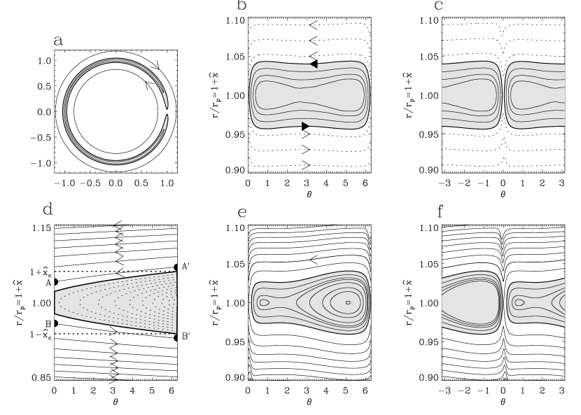
Figure 1: The figures $a$ to $c$ represent the same situation: a $15$ M_⊕ protoplanet embedded in a $4$ % aspect ratio disk, once a steady state has been reached. The details of the run are unimportant here, as these figures are for illustration purpose only, and closely resemble other runs presented elsewhere (see e.g. Masset & Snellgrove 2001, or Nelson et al. 2000). Figure $d$ shows streamlines which fulfill the prescriptions 1 to 3 of section  3.2. The figures $e$ and $f$ represent the same situation, except for a $\pi$-shift in azimuth. The run they are extracted from differs from the run of figures $a$ to $c$ only by the viscosity, which has been set this time to a very high value. In figures $d$ to $f$, the solid line in the outer and inner disk (outside of the shaded –librating– region) represents a unique streamline, which is also, as we are dealing with a steady flow, the path of a fluid element on its way to the central star.

The separatrix between the librating (horseshoe) and circulating (inner and outer disk) streamlines is represented as a thick solid line. The planet lies at $r/r_{p}=1$ and $\theta=0$ (mod. $2\pi$). The circulating streamlines always stay on the same side of the planet’s orbit, as is better seen in Fig. 1c. One can see that these circulating streamlines get deflected as they pass by the planet. This corresponds to the excitation of epicyclic motion and the exchange of angular momentum with the disk, which is carried away by pressure effects and gives rise to the wake, which can be clearly seen in Fig. 1b and 1c. The angular momentum transfer rate into this wake corresponds to the Lindblad torques.

3.2 Viscous case

In order to have a first idea of the streamline topology we approximate the action of the planet on the flow with the following prescription:

1. The planet acts on a fluid element at $\theta=0$ (mod. $2\pi$) only (i.e., at a conjunction).

2. If the distance $|x|$ of the fluid element to the orbit when it is in conjunction with the planet, is smaller than some threshold value $x_{c}$ (which corresponds to the half-width of the horseshoe region), then the fluid element is “reflected” with respect to the planet orbit and sent to $(\theta,-x)$. Otherwise no action is taken on the fluid element. This is meant to mimic the U-turn of the fluid element at the end of the horsestreamlines in the horseshoe region.

3. The fluid element velocity is assumed to be everywhere the velocity in the unperturbed disk.

Obviously this oversimple prescription reproduces in an inviscid case the main properties outlined at the previous section, i.e., it gives rectangular librating streamlines in the horseshoe region (the width of which is $2x_{c}$), and circulating circular streamlines in the outer and inner disk. However there is no wake. In a viscous disk with uniform viscosity and surface density, the fluid element velocity in the corotating frame is given by (if we assume the radial extend of the coorbital region to be small compared to the planet distance):

$$\dot{x}=-\frac{3}{2}\frac{\nu}{r_{p}}\mbox{~{}~{}~{}and~{}~{}~{}}\dot{\theta}=-\frac{3}{2}\frac{\Omega_{p}}{r_{p}}x$$ (1)

which integrates as:

$$\theta=\frac{1}{2}\frac{\Omega_{p}}{\nu}x^{2}+\theta_{0}$$ (2)

The streamlines are therefore arcs of parabola, and the sketch of the streamlines which respect the prescription given above is represented in Fig. 1d. If we follow the path of a fluid element along the solid streamline originating in the outer disk, we see that first this fluid element has a circulating trajectory and approaches progressively the planet coorbital zone. The distance between two successive intersections of the streamline with say the $\theta=0$ axis increases steadily, since the angular frequency mismatch between the planet and the fluid element decreases. When the fluid element reaches the point $A^{\prime}$, it is not sent on the other side of the orbit, since its distance to the planet is still larger than $x_{c}$. However, along the arc $A^{\prime}A$, it crosses the horseshoe region outer boundary, and when it reaches $A$, it is sent to $B$ and therefore gives to the planet, during this close encounter, the positive amount of angular momentum that it loses. It then follows its path along $BB^{\prime}$, which by construction is symmetric to $AA^{\prime}$, therefore when it reaches $B^{\prime}$, it is out of the horseshoe region, and therefore it keeps circulating in the inner disk, and eventually gets accreted onto the primary.

One can wonder how this schematic picture changes in a more realistic case. First it can be useful to notice that in a 2D steady flow defined on a compact domain, a streamline which does not intersect the domain boundaries is closed. Therefore one has to expect a region of closed streamlines behind the planet, which enclose the fixed point on the orbit where the negative viscous torque cancels out the positive torque from the planet, which goes from $0$ to an arbitrarily large value as $\theta$ goes from $\pi$ to $2\pi$, and, if the viscosity is small enough, this closed region should extend from one end to another of the horseshoe region. We represent in Fig. 1e and 1f a situation taken from a run similar to the run of Fig. 1a to 1c, except that the viscosity has been set to a very high value (corresponding to $\alpha\sim 0.1$, which is probably too high for a protoplanetary disk, but has the merit that it clearly shows the streamlines topology). We see on this figure that we have a closed streamlines region which resembles the one obtained with the oversimple prescription, and that material flows from the outer disk to the inner disk.

Therefore, in the case of a finite viscosity, we still have a set of closed librating streamlines in the coorbital region, enclosed by a closed separatrix, which corresponds to trapped material which will not be accreted onto the primary, but now the outer and inner disk communicate, and as material flows from the outer disk to the inner disk it exerts on the planet a positive torque. The smaller the viscosity, the more the librating region has a rectangular shape and resembles the horseshoe region of the inviscid case.

4 Coorbital corotation torque expression

The material enclosed within the separatrix is trapped and therefore its angular momentum is constant with time, since the planet is on a fixed circular orbit. Hence the net torque on the librating region $L$ vanishes. This torque can be decomposed as the gravitational torque exerted by the planet $\Gamma_{p\rightarrow L}$ and the viscous torque $\Gamma^{vis}_{S}$ exerted by the inner and outer disk on $L$ at the separatrix $S$, hence:

$$\Gamma_{p\rightarrow L}+\Gamma^{vis}_{S}=0$$ (3)

In what follows we make the following assumptions:

1. the viscosity is small enough so that the separatrix distance to the orbit is almost constant when one stands far from the horseshoe U-turn regions;

2. the outer and inner separatrices lie at the same distance $x_{s}$ from the orbit. This neglects in particular the mismatch between the orbit and the corotation, due to the fact that the disk is slightly sub-Keplerian (due to the partial support of the central object gravity by a radial pressure gradient). For an aspect ratio of a few percents, this mismatch is typically $10^{-3}r_{p}$, while for the protoplanet masses we consider, $x_{s}\sim$ a few $10^{-2}r_{p}$, and therefore assumption 2 is reasonable. However, when considering disks with aspect ratios $>0.1$, and/or smaller mass planets, this mismatch can no longer be neglected.

3. the perturbed quantities in the librating region are independent of $\theta$, and thus are only function of $x$.

Experience from numerical simulations shows that this last assumption is reasonable; for instance, the shallow ‘dip’ profile that is observed when the mass is sufficiently large and the viscosity is sufficiently low can be considered as independent of $\theta$ with a very good approximation as long as one excludes the U-turn ends of the horseshoe region. We neglect the torque exerted by the inner and outer disk on $L$ at the U-turn ends of the librating region, and we neglect the torque of the pressure forces on $L$. The coorbital corotation torque on the planet, which is the torque exerted by the disk material during the close encounters with the planet, can therefore be expressed, using Eq. (3) as:

$$\Gamma_{C} = \Gamma_{L\rightarrow p}+\Gamma_{R}=\Gamma^{vis}_{S}+\Gamma_{R}{}$$

$$= {}\Gamma^{vis}_{S^{+}}+\Gamma^{vis}_{S^{-}}+\Gamma_{R}$$

where $\Gamma_{L\rightarrow p}=-\Gamma_{p\rightarrow L}$ is the gravitational torque exerted by the librating region on the planet, $\Gamma_{R}$ is the torque exerted on the planet by the circulating material when it flows from the outer disk to the inner disk, $\Gamma^{vis}_{S^{+}}$ is the torque exerted by the outer disk on the librating region at the outer separatrix, and $\Gamma^{vis}_{S^{-}}$ is the torque exerted by the inner disk on the librating region at the inner separatrix. We can write:

$$\Gamma^{vis}_{S^{\pm}}=\mp 2\pi\nu(r_{p}\pm x_{s})^{2}\Sigma_{S^{\pm}}\left[-\frac{3}{2}\Omega+\left(\frac{\partial v}{\partial r}\right)\right]_{r_{p}\pm x_{s}}$$ (5)

and:

$$\Gamma_{R}=\dot{M}[j(r_{p}+x_{s})-j(r_{p}-x_{s})]$$ (6)

where $\dot{M}$ is the mass flow from the outer disk to the inner disk, which would be $3\pi\nu\Sigma_{\infty}$ in a strictly stationary regime, and where we have assumed: $|\partial v/\partial r|\gg|v/r|$. To lowest order in $x_{s}/r_{p}$, Eq. (6) can be recast as:

$$\Gamma_{R}=\dot{M}[\Omega_{p}r_{p}x_{s}+2(r_{p}+x_{s})v_{+}-2(r_{p}-x_{s})v_{-}]$$ (7)

where $v_{\pm}$ is the perturbed azimuthal velocity at the outer (resp. inner) separatrix. Therefore, the use of Eqs. (4), (5) and (7) enables one to estimate the corotation torque only from the knowledge of the unperturbed disk characteristics and the flow properties at the separatrix, provided a steady flow solution is known, since the steady flow assumption is necessary to write Eq. (3).

5 Steady state solution

In order to find a steady state solution, we write a radial viscous iffusion equation for the surface density. This equation needs to include the turnover of the horseshoe orbits. One simple way to do that is to include source and sink terms for $|x|<x_{s}$. This is detailed in Appendix A.

When this steady flow solution is used to evaluate the torque expression given by Eqs. (4), (5) et (7), in which we neglect the perturbed azimuthal velocity profile and the even part in $x$ of the density profile perturbation (the ‘dip’ which surrounds the orbit), one obtains:

$$\Gamma_{C}=\frac{9}{2}x_{s}^{4}\Omega_{p}^{2}\Sigma_{\infty}{\cal F}(z_{s})$$ (8)

where:

$${\cal F}(z_{s})=\frac{1}{z_{s}^{3}}-\frac{g(z_{s})}{z_{s}^{4}g^{\prime}(z_{s})}$$ (9)

where $g$ is a linear combination of the Airy functions Ai and Bi defined by Eq. (A18) and where:

$$z_{s}=x_{s}\left(\frac{\Omega_{p}}{2\pi\nu r_{p}}\right)^{1/3}$$ (10)

In particular, in the highly viscous case ($z_{s}\ll 1$), we have:

$$\Gamma_{C}=\frac{9}{8}x_{s}^{4}\Omega_{p}^{2}\Sigma_{\infty}$$ (11)

where we use the fact that (Abramowitz & Stegun, 1972):

$$\frac{g(t)}{g^{\prime}(t)}=t-\frac{1}{4}t^{4}+o(t^{4})$$ (12)

Eq. (11), with our notations, is the same as the expression given by Ward (1992):

$$\Gamma_{C}^{\prime}=\frac{3}{4}x_{s}^{4}\Omega_{p}^{2}\Sigma_{\infty}\left(\frac{3}{2}-\beta\right)$$ (13)

in which we have to set the slope $\beta=-d\log\Sigma/d\log r$ to $0$ since we are in the very viscous regime in a uniform surface density disk.

In the general case, at lower viscosities, there is an ambiguity in the choice of the slope of $\beta$ that has to be used in Eq. (13). Indeed, if we choose:

$$\beta_{1}=-\frac{d\Sigma}{dx}\frac{r_{p}}{\Sigma_{\infty}}\mbox{~{}~{}~{}at $\hat{x}=0$}$$ (14)

then we get the expression:

$$\Gamma_{C_{1}}^{\prime}=\frac{9}{8}x_{s}^{4}\Omega_{p}^{2}\Sigma_{\infty}\frac{g(z_{s})}{z_{s}g^{\prime}(z_{s})}$$ (15)

whereas if we choose:

$$\beta_{2}=-\frac{\Sigma(x_{s})-\Sigma(-x_{s})}{2x_{s}}\frac{r_{p}}{\Sigma_{\infty}}$$ (16)

then we get:

$$\Gamma_{C_{2}}^{\prime}=\frac{9}{8}x_{s}^{4}\Omega_{p}^{2}\Sigma_{\infty}\frac{g^{\prime}(0)}{g^{\prime}(z_{s})}$$ (17)

The graphs of $\Gamma_{C}$, $\Gamma_{C_{1}}^{\prime}$ and $\Gamma_{C_{2}}^{\prime}$ are represented in Fig. 2. $\Gamma_{C_{1}}^{\prime}$ is always smaller than $\Gamma_{C}$, and $\Gamma_{C_{2}}^{\prime}$ is always larger than $\Gamma_{C}$. This means that it is always possible to find a value for $\beta$ between $\beta_{1}$ and $\beta_{2}$ for which Eqs. (8) and (13) give the same value.

Figure 2: Coorbital corotation torque as a function of viscosity. The solid curve is a plot of expression (8), while the dashed and dotted ones represent respectively Eqs. (15) and (17). Here $\Gamma_{C}^{max}$ stands for $\frac{9}{8}\Omega_{p}^{2}x_{s}^{4}\Sigma_{\infty}$.

The ambiguity in the choice of $\beta$ for Eq. (13) comes on one hand from the fact that this equation has been derived by an integration of the torque on all the librating streamlines of the horseshoe region, and on the other hand from the fact that the solution of Eq. (A17) does not lead to a constant slope over the whole horseshoe region. Such an ambiguity does not exist in Eq. (8) since this latter has been derived taking into account only the disk perturbation at the separatrix. What happens in the interior of the librating region does not need to be known, provided we are dealing with a steady flow.

The ratio ${\cal R}=\nu r_{p}/(\Omega_{p}x_{s}^{3})=1/(2\pi z_{s}^{3})$ is also $\frac{1}{8\pi}\frac{\tau_{HS}}{\tau_{visc}}$, where:

$$\tau_{HS}=\frac{4\pi r_{p}}{\frac{3}{2}\Omega_{p}x_{s}}$$ (18)

and:

$$\tau_{visc}=\frac{x_{s}^{2}}{3\nu}$$ (19)

are respectively the turnover time of the outermost horseshoe orbit and the viscous diffusion time across the horseshoe region. From Fig. 2 we see that the coorbital corotation torque reaches half of its maximum value at ${\cal R}=\hat{\nu}/\hat{x}_{s}^{3}\sim 0.05$, that is to say for $\tau_{HS}\sim\tau_{visc}$. When the turnover time is much larger than the viscous time, i.e. when ${\cal R}\gg 0.05$, the corotation torque reaches its maximal value, since libration is inefficient at removing the vortensity gradient. On the contrary, when the viscous time is much larger than the turnover time (i.e., when ${\cal R}\ll 0.05$) libration can remove the vortensity gradient and the corotation torque has a negligible value.

5.1 Cut-off at high viscosity

As discussed in section 3.2, the outer separatrix can be approximated as a branch of parabola in the $\theta,r$ plane, and so far we have assumed that the viscosity is small enough so that we can approximate the separatrix by a line of constant distance to the orbit. However, if the viscosity is very high this is no longer true, and the separatrix can reach the orbit before having described a complete revolution in the planet frame. From Eq. (2), we can give an estimate of the critical value for the viscosity above which this will happen, by setting $\theta_{0}=0$, $x=x_{s}$ and $\theta=2\pi$. This leads to:

$$\nu_{c}=\frac{x_{s}^{2}\Omega_{p}}{4\pi}$$ (20)

The 2D analysis we have developed here is mainly valid for mildly embedded protoplanets, for which the Hill radius is a sizable amount of the disk thickness; this would correspond to values of the $\alpha$-parameter of about $\alpha\sim 0.1$, probably too high for protoplanetary disks, and therefore this regime is not very relevant for the analysis described in this paper.

6 Additional terms and Lindblad torque coupling

The coorbital corotation torque general expression in a steady regime, which we have given in Eqs. (4), (5) and (7), contains additional terms that we have so far neglected. In the following we still neglect the terms linked to the perturbed azimuthal velocity $v$, the analysis of which will be found in Appendix B, but we do not neglect, as we have done before, the perturbation of the density profile in the vicinity of the planet orbit. Indeed, as is seen frequently in numerical simulations, the mildly embedded planets, which are not massive enough to fulfill the gap opening criteria, are nevertheless surrounded by a shallow axisymmetric depletion of their coorbital region. As a consequence, a new term arises in the torque expression, which reads:

$$\Gamma_{C}^{I}=3\pi\nu(\Sigma_{\infty}-\Sigma_{s})\cdot\Omega_{p}r_{p}x_{s}$$ (21)

where $\Sigma_{s}$ is the average of the surface density at the outer and inner separatrices (in different words it is the value of the even part in $\hat{x}$ of the perturbed density, sampled at any separatrix). If we assume that this value is the same as the value at the orbit (which means that the dip edges lie further from the orbit than the separatrix), then we can write:

$$\Sigma_{\infty}-\Sigma_{S}=\frac{\Gamma_{LR}}{3\pi\nu\Omega_{p}r_{p}^{2}}$$ (22)

where $\Gamma_{LR}>0$ is the one-sided Lindblad torque. Eq. (22) is obtained by equating the viscous torque and the torque given by the wake damping, and integrating it between the orbit and an outer radius where most of the wave angular momentum has been transfered to the disk (i.e., it is obtained by integrating twice the even part in $x$ of Eq. (A) in the steady state case). Because of this integration, the assumption of local damping is not necessary in writing Eq. (22). However, the damping must occur over a radial range smaller than the planet orbital radius for this expression to be accurate. Recent work by Goodman & Rafikov (2000) shows that this may be indeed the case even for relatively small planet masses. Using Eq. (22), the torque expression of Eq. (21) can be recast as:

$$\Gamma_{C}^{I}=\frac{x_{s}}{r_{p}}\Gamma_{LR}$$ (23)

It can be argued that this result has been obtained assuming a strictly steady flow, and in particular that the mass flow from the outer disk to the inner disk across the planet orbit is exactly $3\pi\nu\Sigma_{\infty}$. A higher mass rate than this value (which is $3\pi\nu\Sigma_{\infty}$ either far from the planet or in the unperturbed disk) would lead to a value for $\Gamma_{C}^{I}$ higher than the one given by Eq. (23). The analytical work for an inviscid disk by Lubow (1990), and Goodman & Ravikov (2000), as well as numerical evaluation of the mass flow rate accross the orbit of a non-accreting protoplanet (Masset and Snellgrove, 2001, in their Fig. 4) suggest that the actual mass flow rate across corotation is higher than $3\pi\nu\Sigma_{\infty}$, and that the difference between the actual value and $3\pi\nu\Sigma_{\infty}$ scales with $\Sigma_{\infty}M_{p}^{2}$. This issue definitely requires further work, as it could provide another positive additional term to the corotation torque.

The other terms which appear in the general torque expression are evaluated in B. They all correspond to the difference between the outer and the inner separatrix of quantities involving the perturbed azimuthal velocity $v$. The perturbed azimuthal velocity can be split in two parts: the part which corresponds to the disk axisymmetric profile perturbation under the action of the Lindblad torques, which is odd in $x$ to lowest order in the disk aspect ratio, and an even part in $x$ (to lowest order in $\hat{x}_{s}$), which corresponds to the odd perturbation density due to libration that we have analyzed at Appendix A. However in the analysis of Appendix A we have neglected the perturbation of the azimuthal velocity, and therefore we cannot estimate the additional terms linked to the even component of the perturbed azimuthal velocity. Taking this latter into account would have led to a higher order diffusion equation in Eq. (A) which would have involved the disk thickness, which has not been considered in the simple analysis of Appendix 5. This will be done in a forthcoming work. We note that the additional term linked to this even component of the perturbed azimuthal velocity may play a non negligible role and significantly modify the viscosity dependent part of the corotation torque given by Eq. (8).

The additional term linked to the odd component of the perturbed azimuthal velocity depends only on the value of this latter at the separatrix. However, one can only give a rough estimate of the maximal value of these terms. Their actual value will depend on the exact position at which the separatrix samples the perturbed velocity profile. It turns out that the maximal value of this term is of the same order of magnitude as the additional term of Eq. (23):

$$\Gamma_{C}^{II}\leq\frac{2}{3}\frac{x_{s}}{r_{p}}(2-\beta)\Gamma_{LR}$$ (24)

Hence we see that the main effect of the additional terms (both $\Gamma_{C}^{I}$ and $\Gamma_{C}^{II}$) is to introduce a coupling with the one-sided Lindblad torque, as they add a small, positive fraction of this latter to the coorbital corotation torque. Now, the differential Lindblad torque is a small, negative fraction of the one-sided Lindblad torque, which scales with the aspect ratio (for instance in the disk we consider, with a uniform surface density and a constant aspect ratio $h^{\prime}$, $\Delta\Gamma_{LR}\approx-8h^{\prime}\Gamma_{LR}$). Therefore this additional term plays against the differential Lindblad torque and one has to expect that the migration is considerably slower than standard type I migration estimates, or even reversed, over a certain planet mass range, in very thin viscous disks. The exact determination of this mass range has to be achieved through numerical simulations, since the analytical determination of the exact perturbed density profile, of the exact azimuthal perturbed velocity profile, and of the exact separatrix position seems a hardly tractable task.

7 Discussion

We have derived the expression of the coorbital corotation torque exerted by a uniform viscosity and surface density disk on an embedded protoplanet on a fixed circular orbit, assuming a 2D steady flow in the planet frame. We have obtained the following expression for the torque:

$$\Gamma_{C}=\frac{9}{2}x_{s}^{4}\Omega_{p}^{2}\Sigma_{\infty}{\cal F}(z_{s})+\frac{x_{s}}{r_{p}}{\cal G}(x_{s})\Gamma_{LR}$$ (25)

where ${\cal F}(z_{s})$ is given by Eq. (9), and where ${\cal G}(x_{s})$ is a function of the order of unity, the exact value of which depends on the position of the separatrix and of the perturbed axisymmetric profile of the disk under the action of the Lindblad torques, and the maximum value of which is $7/3$, as can be inferred from Eqs. (23) and (24). The first term in the R.H.S. of Eq. (25) corresponds to previous estimates of the corotation torque, and exhibits an explicit dependence on the viscosity: when the viscous diffusion timescale across the coorbital region is larger than the horseshoe libration time, this term is negligible, while when the viscous diffusion time is shorter than the libration time, it reaches its maximum value. The second term of the R.H.S. of Eq. (25) comes from a dependence of the viscous torque acting on the boundary (separatrix) of the trapped librating region on the perturbed axisymmetric profile of the disk under the action of the one-sided Lindblad torques on each side of the orbit. This term slows down the migration and could even reverse it in sufficiently thin disks.

This analysis is valid as long as the flow around the planet can be considered as a 2D steady flow. Therefore the planet Hill radius needs to be a sizable amount of the disk thickness, and gas accretion cannot occur onto the planet (otherwise the flow cannot be considered as steady if the accretion time is short, and the separatrix splits into two lines which enclose the band of the material which is going to be accreted; see e.g., Lubow et al. 1999). Therefore the mass limit for this analysis is roughly $15$ $M_{\oplus}$. Another condition for the analysis presented above to be valid is that the planet does not open a gap in the disk (otherwise the corotation torque is negligible). The depletion which appears around the planet orbit and which leads to the Lindblad torque coupling needs to be shallow.

The analysis presented here relies on the existence of a viscous drift of the disk material across the planet orbit. Therefore it can apply to those parts of the disk where MHD turbulence occurs and leads to an effective viscosity (Balbus & Hawley, 1991). Hence it is likely to apply mainly to the innermost part of the protoplanetary disks (the central astronomical unit). It is questionable whether this kind of turbulent transport can be correctly modeled by an effective viscosity when applied to the disk-planet angular momentum exchange in the coorbital region. In particular the steady state assumption that was used to estimate the corotation torque needs to be reconsidered.

One may speculate about the extrapolation of the calculations exposed here to smaller masses, for which the Hill radius is much smaller than the disk thickness (deeply embedded planets). However the 2D flow assumption was essential for the identification of a closed region of trapped material. There is no guarantee that we could perform the same kind of calculation in the 3D case. However, if the planet has no inclination and no eccentricity, the gas motion in the disk equatorial plane would still be 2D for symmetry reasons, and therefore would have a set of closed streamlines in the steady state regime. However, the extension of the trapped region above the equatorial plane would need to be discussed.

In the case of a finite excentricity, the analysis exposed here is no longer valid; in particular, the planet and the disk can exchange angular momentum at the excentric corotation resonance locations, which are not localized where the disk material corotates with the planet guiding center (i.e., which do not lie at the orbit semi-major axis, if one neglects the radial pressure gradient as a partial support to gravity in the disk). However, it would be interesting to find a link between the torque expression obtained by summing over the resonances and an analysis similar to the one exposed above, in which the separatrix would become a band of width $2ea$ (using the fact that the epicyclic frequency is much higher than the outermost horseshoe turnover frequency). In particular it would be of interest to see how the coupling with the one-sided Lindblad torque is modified by the introduction of a finite excentricity.

This analysis needs to be extended to the case of an arbitrary surface density profile, and to a migrating planet (for which the mass flow across the orbit will therefore differ from $3\pi\nu\Sigma_{\infty}$). In this case the corotation torque would include a delayed term proportional to $\dot{a}$, the planet drift rate, and would lead to a feedback on the migration. This will be presented in a forthcoming work.

Appendix A Steady flow solution

In the horseshoe region we write the continuity equation integrated over an arc of a ring $[r,r+\delta r]$ which excludes the horseshoe U-turn ends of the streamlines. We are led to:

$$\frac{\partial\Sigma}{\partial t}+\frac{1}{r}\frac{\partial(\Sigma ur)}{\partial r}-\frac{1}{2\pi}\left(\frac{r^{\prime}}{r}|\Omega_{p}-\Omega^{\prime}|\Sigma^{\prime}\frac{\delta r^{\prime}}{\delta r}-|\Omega_{p}-\Omega|\Sigma\right)=0$$ (A1)

where $u$ is the radial velocity. In Eq. (A1) we assume that the arc of ring spans almost an angle $2\pi$, and that it is mapped, after a horseshoe U-turn, onto the arc of ring of radius $r^{\prime}$ and width $\delta r^{\prime}$. We also neglect the perturbed azimuthal velocity. The variables $\Sigma^{\prime}$ and $\Omega^{\prime}$ stand respectively for $\Sigma(r^{\prime})$ and $\Omega(r^{\prime})$. The left term of the bracket corresponds to the mass which comes from ‘the other side’ (i.e., the ring $[r^{\prime},r^{\prime}+\delta r^{\prime}]$), and enters the ring $[r,r+\delta r]$ after a horseshoe U-turn, while the second term in this bracket corresponds to the mass which leaves the ring $[r,r+\delta r]$.

The torque per unit mass $T$ acting on the disk material can be decomposed as the sum of the viscous torque per unit mass and the torque per unit mass $(2\pi R\Sigma)^{-1}d\Gamma/dr$ arising from the wake damping:

$$T=\frac{1}{r\Sigma}\frac{\partial(r^{3}\nu\Sigma\frac{d\Omega}{dr})}{\partial r}+\frac{1}{2\pi R\Sigma}\frac{d\Gamma}{dr}$$ (A2)

Writing $T=u\partial j/\partial r=u\partial j_{0}/\partial=ur\Omega/2$, and using Eqs. (A1) and (A2), one is led to the following radial diffusion equation:

$$\frac{\partial\Sigma}{\partial t} = \frac{1}{2\pi}\left(\frac{r^{\prime}}{r}|\Omega_{p}\right.-\Omega^{\prime}|\Sigma^{\prime}\frac{\delta r^{\prime}}{\delta r}{}{}-|\Omega_{p}-\Omega|\Sigma^{\prime}\left)\Pi\left(\frac{|x|}{x_{s}}\right)+3\nu\frac{\partial^{2}\Sigma}{\partial r^{2}}\right.-\frac{1}{\pi r^{2}\Omega}\frac{d^{2}\Gamma}{dr^{2}}$$ (A3)

where $\Pi$ is defined as:

$$\begin{array}[]{ccl}\Pi:u&\longmapsto&1\mbox{~{}~{}if $|u|<1$}\\ &&0\mbox{~{}~{}otherwise}\end{array}$$

and accounts for the fact that the source and sink terms are present only over the horseshoe region (i.e. $|x|<x_{s}$). In Eq. (A3) we have assumed $r|\partial^{2}\Sigma/\partial r^{2}|\gg|\partial\Sigma/\partial r|$ and $r|d^{2}\Gamma/dr^{2}|\gg|d\Gamma/dr|$. If we neglect both pressure and viscous effects during a U-turn at one end of the horseshoe orbit, then the conservation of the Jacobi constant of a fluid element implies, as has been shown by Ward (1992), that:

$$\frac{\delta r}{\delta r^{\prime}}=\frac{r^{\prime}B^{\prime}|\Omega^{\prime}-\Omega_{p}|}{rB|\Omega-\Omega_{p}|}$$ (A4)

where $B$, the second Oort’s constant, in the case of a Keplerian disk, is also $B=\Omega/4$. Using Eq. (A3) and (A4), one can write:

$$\frac{\partial\Sigma}{\partial t} = \frac{1}{2\pi}\left(\Sigma^{\prime}\frac{\Omega}{\Omega^{\prime}}-\Sigma\right)|\Omega_{p}-\Omega|\Pi\left(\frac{|x|}{x_{s}}\right)+3\nu\frac{\partial^{2}\Sigma}{\partial r^{2}}-\frac{1}{\pi r_{p}^{2}\Omega_{p}}\frac{d^{2}\Gamma}{dr^{2}}$$ (A5)

If we write $x^{\prime}=r^{\prime}-r_{p}$, and if we define the dimensionless distances to the orbit as $\hat{x}=x/r_{p}$ and $\hat{x}^{\prime}=x^{\prime}/r_{p}$, then we have:

$$\frac{\Omega}{\Omega^{\prime}}=1-\frac{3}{2}\hat{x}+\frac{3}{2}\hat{x}^{\prime}+\frac{15}{8}\hat{x}^{2}+\frac{3}{8}\hat{x}^{\prime 2}+O(\hat{x}^{3})+O(\hat{x}^{\prime 3})$$ (A6)

From Eq. (A4), we can infer that $\hat{x}=-\hat{x}^{\prime}$ to lowest order in $\hat{x}$, therefore:

$$\hat{x}^{\prime}=-\hat{x}+\zeta\hat{x}^{2}+O(\hat{x}^{3})$$ (A7)

where $\zeta$ is a numerical constant. Hence the bracket in the source term of Eq. (A5) reads:

$$\Sigma^{\prime}\frac{\Omega}{\Omega^{\prime}}-\Sigma = \Sigma(-\hat{x})-\Sigma(\hat{x})-3\hat{x}\Sigma(-\hat{x}){}$$

$${}+\frac{1}{4}(9+6\zeta)\hat{x}^{2}\Sigma(-\hat{x})+\zeta\hat{x}^{2}\frac{\partial\Sigma}{\partial\hat{x}}(-\hat{x})+O(\hat{x}^{3})$$

If we keep only terms to first order in $\hat{x}$ in this expression, Eq. (A5) can be recast as:

$$\frac{\partial\Sigma}{\partial t} = \frac{3}{4\pi}\Omega_{p}[\Sigma(-\hat{x})-\Sigma(\hat{x})-3\hat{x}\Sigma(-\hat{x})]{}$$

$${}\times\left(1-\frac{5}{4}\hat{x}\right)|\hat{x}|\Pi\left(\frac{\hat{x}}{\hat{x}_{s}}\right)+\frac{3\nu}{r_{p}^{2}}\frac{\partial^{2}\Sigma}{\partial\hat{x}^{2}}-\frac{1}{\pi r_{p}^{4}\Omega_{p}}\frac{d^{2}\Gamma}{d\hat{x}^{2}}+O(\hat{x}^{3})$$

We call $\tilde{\Sigma}$ and $\check{\Sigma}$ respectively the odd and even part in $\hat{x}$ of $\Sigma$:

$$\left\{\begin{array}[]{rcl}\tilde{\Sigma}(\hat{x})&=&\frac{1}{2}[\Sigma(\hat{x})-\Sigma(-\hat{x})]\\ \check{\Sigma}(\hat{x})&=&\frac{1}{2}[\Sigma(\hat{x})+\Sigma(-\hat{x})]\end{array}\right.$$

We write $\check{\Sigma}(\hat{x})=\Sigma_{c}+O(\hat{x}^{2})$, where $\Sigma_{c}=\check{\Sigma}(0)=\Sigma(0)$. Taking the odd part in $\hat{x}$ of both sides of Eq. (A), and keeping terms only up to $O(\hat{x}^{2})$, one is led to:

$$\frac{\partial\tilde{\Sigma}}{\partial t} = -\frac{3}{4\pi}\Omega_{p}|\hat{x}|\Pi\left(\frac{\hat{x}}{\hat{x}_{s}}\right)[2\tilde{\Sigma}(\hat{x})+3\hat{x}\Sigma_{c}]+\frac{3\nu}{r_{p}^{2}}\frac{\partial^{2}\tilde{\Sigma}}{\partial\hat{x}^{2}}$$ (A10)

where we have neglected, at this step, the Inner and Outer Lindblad torque imbalance, and thus the odd part in $\hat{x}$ of $\Gamma$ and its second derivative vanishes. We write $s=\tilde{\Sigma}/\Sigma_{c}$ and $\hat{\nu}=\nu/(r_{p}^{2}\Omega_{p})$, and we assume that we have a steady state. Therefore, for $\hat{x}>0$, we have:

$$\hat{\nu}\frac{\partial^{2}s}{\partial\hat{x}^{2}} = \frac{1}{4\pi}[2s+3\hat{x}]\hat{x}\mbox{~{}~{}if $\hat{x}<\hat{x}_{s}$}$$

$$= {}0\mbox{~{}~{}otherwise}$$

The first line of Eq. (A) shows the balance between libration, which tends to create a profile of density such that $s=-\frac{3}{2}\hat{x}$, and the viscous diffusion. We want to find a solution to this ODE valid for any $\hat{x}>0$, and such that $s(0)=0$, since $s$ is an odd function of $x$.

The general solution of Eq. (A) for $\hat{x}>\hat{x}_{s}$ is $s=a\hat{x}+b\hat{x}^{2}$, which does not diverge for large values of $\hat{x}$ only if $a=0$ and $b=0$. Therefore, we are led to seek a solution of Eq. (A) for $\hat{x}\in[0,\hat{x}_{s}]$ which fulfills the two conditions:

$$\left\{\begin{array}[]{rcl}s(0)&=&0\\ s^{\prime}(\hat{x}_{s})&=&0\end{array}\right.$$ (A12)

where $s^{\prime}\equiv\partial s/\partial\hat{x}$. If we define

$$S=s+\frac{3}{2}\hat{x}$$ (A13)

and

$$z=(2\pi\hat{\nu})^{-1/3}\hat{x},$$ (A14)

then Eq. (A) can be recast, for $0<z<z_{s}=(2\pi\hat{\nu})^{-1/3}\hat{x}_{s}$, as:

$$\frac{\partial^{2}S}{\partial z^{2}}=zS$$ (A15)

and the set of conditions (A12) becomes:

$$\left\{\begin{array}[]{rcl}S(0)&=&0\\ \frac{\partial S}{\partial z}(z_{s})&=&\frac{3}{2}(2\pi\hat{\nu})^{\frac{1}{3}}\end{array}\right.$$ (A16)

The solution of Eq. (A15) which fulfills the conditions (A16) is:

$$S(z)=\frac{3(2\pi\hat{\nu})^{1/3}}{2g^{\prime}(z_{s})}g(z)$$ (A17)

where:

$$g(z)=\frac{\mbox{Bi}(z)-\sqrt{3}\mbox{Ai}(z)}{2\mbox{Bi}^{\prime}(0)}$$ (A18)

is the linear combination of Airy functions Ai and Bi such that $g(0)=0$ and $g^{\prime}(0)=1$. This solution can be used to evaluate the coorbital corotation torque given by the expressions (4), (5) and (7). In this part we neglect the perturbed azimuthal velocity, and we neglect as well the even part of the density profile perturbation (the shallow ‘dip’) which appears around the orbit for a sufficient mass (i.e., we write $\check{\Sigma}\equiv\Sigma_{\infty}$). Furthermore we assume that the mass flow across the coorbital region from the outer disk to the inner disk is $\dot{M}=3\pi\nu\Sigma_{\infty}$. Therefore the expression of the corotation torque, in this approximation, reduces to:

$$\Gamma_{C} = 3\pi\nu[(r_{p}-x_{s})^{2}\Omega(r_{p}+x_{s})^{2}\Sigma_{S^{+}}{}$$

$${}-(r_{p}-x_{s})^{2}\Omega(r_{p}-x_{s})\Sigma_{S^{-}}]$$

$${}+3\pi\nu\Sigma_{\infty}[j_{0}(r_{p}+x_{s})-j_{0}(r_{p}-x_{s})]$$

which leads to:

$$\Gamma_{C}=-6\pi\nu r_{p}^{2}\Omega_{p}\Sigma_{\infty}s(\hat{x}_{s})$$ (A20)

Using Eqs. (A13), (A17) and (A20), one can finally deduce Eq. (8).

Appendix B Additional terms

The additional term arising from the even part in $\hat{x}$ of $\partial v/\partial r$ in Eq. (5) reads:

$$\Gamma_{C}^{II}=4\pi\nu r_{p}x_{s}\Sigma_{c}\left(\frac{\partial v}{\partial r}\right)_{S+}(2-\beta)$$ (B1)

where $\Sigma_{c}$ is the surface density at the planet orbit.

In order to give an estimate of $v$, we write the axisymmetric part of the linearized radial Euler equation, in which we omit the gradient of the $m=0$ perturbed potential of the planet. This reads:

$$2\Omega v-c_{s}^{2}\frac{\partial_{r}\Sigma}{\Sigma_{\infty}}=0$$ (B2)

where $c_{s}$ is the sound speed. We can give a maximal estimate of $\partial_{r}\Sigma$ by writing that the wave damping occurs over a radial range of at least one disk thickness. This reads:

$$3\pi\nu\Omega r^{2}\frac{\partial\Sigma}{\partial r}\leq\frac{\Gamma_{LR}}{h}$$ (B3)

Using Eqs. (B2) and (B3) one infers:

$$v\leq\frac{h}{6\pi\nu\Sigma_{\infty}r^{2}}\Gamma_{LR}$$ (B4)

In the same manner one can write an upper limit for the perturbed azimuthal velocity derivative: $\partial_{r}v\leq v/h$. Therefore:

$$\frac{\partial v}{\partial r}\leq\frac{\Gamma_{LR}}{6\pi\nu\Sigma_{\infty}r^{2}}$$ (B5)

Assuming that $\Sigma_{c}\simeq\Sigma_{\infty}$, i.e., the dip surrounding the planet orbit is shallow, one can infer from Eqs. (B1) and (B5) that:

$$\Gamma_{C}^{II}\leq\frac{2}{3}(2-\beta)\frac{x_{s}}{r_{p}}\Gamma_{LR}$$ (B6)

The additional term arising from $v$ in Eq. (6) reads:

$$\Gamma_{C}^{III}=3\pi\nu\Sigma_{\infty}\cdot 2x_{s}v$$ (B7)

Using Eq. (B4), one finds as a maximal value for this term:

$$\Gamma_{C}^{III}\leq\frac{x_{s}h}{r_{p}^{2}}\Gamma_{LR}$$ (B8)

Since $h\ll r_{p}$ and $x_{s}\ll r_{p}$, this term is negligible.

References

- (1) Abramowitz, M. and Stegun, I.A. 1972, Handbook of Mathematical Functions, Wiley-Interscience Publication, John Wiley & Sons, New York
- (2) Balbus, S.A. and Hawley, J.F. 1991, ApJ, 376,214
- (3) Goldreich, P. and Tremaine, S. 1980, ApJ, 241, 452
- (4) Goldreich, P. and Tremaine, S. 1979, ApJ, 233, 857
- (5) Goodman, J. and Rafikov, R.R. 2000, astro-ph/0010576
- (6) Korycanski, D.G. and Pollack, J.B. 1993, Icarus, 102, 150
- (7) Lubow, S.H., Seibert, M. and Artymowicz, P. 1999, ApJ, 526, 1001
- (8) Lubow, S.H., 1990, ApJ, 362, 395
- (9) Masset F.S. and Snellgrove, M.D. 2000, MNRAS, in press
- (10) Meyer-Vernet, N. and Sicardy, B. 1987, Icarus, 69, 157
- (11) Nelson, R.P., Papaloizou, J.C.B., Masset, F. and Kley W. 2000, MNRAS, 318, 18
- (12) Papaloizou, J.C.B. and Terquem, C. 1999, ApJ, 521, 823
- (13) Papaloizou, J.C.B. and Lin, D.N.C. 1984, ApJ, 285, 818
- (14) Pollack, J.B., Hubickyj, O., Bodenheimer, P., Lissauer, J.J. , Podolak, M. and Greenzweig, Y. 1996, Icarus, 124, 62
- (15) Shakura, N.I. and Sunyaev, R.A. 1973, A&A, 24, 337
- (16) Ward, W.R. 1997, Icarus, 126, 261
- (17) Ward, W.R. 1992, Abstracts of the Lunar and Planetary Science Conference, vol. 23, 1491
- (18) Ward, W.R. 1991, Abstracts of the Lunar and Planetary Science Conference, vol. 22, 1463
- (19) Ward, W.R. 1986, Icarus, 67, 164