Line-driven winds, ionizing fluxes and UV-spectra of hot stars at extremely low metallicity. I. Very massive O-stars

Abstract

Wind models of very massive stars with metallicities in a range from $10^{-4}$ to 1.0 solar are calculated using a new treatment of radiation driven winds with depth dependent radiative force multipliers and a comprehensive list of more than two million of spectral lines in NLTE. The models are tested by a comparison with observed stellar wind properties of O stars in the Galaxy and the SMC. Satisfying agreement is found. The calculations yield mass-loss rates, wind velocities, wind momenta and wind energies as a function of metallicity and can be used to discuss the influence of stellar winds on the evolution of very massive stars in the early universe and on the interstellar medium in the early phases of galaxy formation. It is shown that the normal scaling laws, which predict stellar mass-loss rates and wind momenta to decrease as a power law with metal abundance break down at a certain threshold. Analytical fit formulae for mass-loss rates are provided as a function of stellar parameters and metallicity.

Ionizing fluxes of hot stars depend crucially on the strengths of their stellar winds, which modify the absorption edges of hydrogen and helium (neutral and ionized) and the line blocking in the far UV. The new wind models are therefore also applied to calculate ionizing fluxes and observable spectra of very massive stars as a function of metallicity using the new hydrodynamic, non-LTE line-blanketed flux constant model atmosphere code developed by Pauldrach et al. (2001). Numbers of ionizing photons for the crucial ionization stages are given. For a fixed effective temperature the He II ionizing emergent flux depends very strongly on metallicity but also on stellar luminosity. A strong dependence on metallicity is also found for the C III, Ne II and O II ionizing photons, whereas the H I and He I ionizing flux is almost independent of metallicity. We also calculate UV spectra for all the models and discuss the behaviour of significant line features as a function of metallicity.

1 Introduction

There is growing evidence that the evolution of galaxies in the early universe was heavily influenced by the formation of first generations of very massive stars. Numerical simulations indicate that for metallicities $Z/Z_{\odot}$ of the order of $10^{-3}$ or smaller the formation of stars with masses larger than 100 M_⊙ is strongly favored and that the Initial Mass Function becomes top-heavy and deviates significantly from the standard (Salpeter) power-law Abel et al. (2000), Abel et al. (2002), Bromm et al. (1999), Bromm et al. (2001a), Bromm et al. (2002a), Nakamura and Umemura (2001). Such an early population of very massive stars at very low metallicities could contribute significantly to the ionization history of the intergalactic medium (Carr et al. 1984, Couchman et al. 1986, Haiman et al. 1997, Bromm et al. 2001b), which appears to have been reionized at redshifts z possibly larger than 6, as the recent work on quasars (Becker et al. 2001, Djorgovski et al. 2001a, Fan et al. 2000, Fan et al. 2002) and Ly_α-emitters (Hu et al. 2002) indicates. Very massive stars are also very likely the progenitors of Gamma-Ray bursts (Mac Fayden et al. 2001, Djorgovski et al. 2001b, Kulkarni et al. 2000, Reichardt 2001), which then - as tracers of the cosmic star formation history - might originate to a large fraction at very high reshift (Bromm et al. 2002b, Ciardi et al. 2000, Lamb et al. 2000). In addition, the extreme Lyman $\alpha$ emitting galaxies at high red redshift can be explained by an ionizing population of very massive stars at very low metallicity (Kudritzki and Puls 2000, Rhoads and Malhotra 2002, Malhotra and Rhoads 2002).

In order to be able to make more quantitative predictions about the influence of such an extremely metal-poor population of very massive stars on their galactic and intergalactic environment, one needs to determine their physical properties during their evolution. A key issue in this regard is the knowledge about their stellar winds.

All hot massive stars have winds driven by radiation. These winds have substantial effects on the structure of the radiating atmospheres. They dominate the density stratification and the radiative transfer through the presence of their macroscopic transonic velocity fields (see Kudritzki 1998 for a detailed review) and they modify the amount of the emergent ionizing radiation significantly (Gabler et al. 1989, Gabler et al. 1991, Gabler et al. 1992, Najarro et al. 1996). Winds have an extremely important influence on the evolution of massive stars by reducing the stellar mass continuously and by affecting evolutionary time-scales, chemical profiles, surface abundances and luminosities. Providing a significant input of mechanical and radiative momentum and energy into the ISM together with the injection of nuclear processed material they can also play a crucial role for the evolution of galaxies. Last but not least, stellar winds provide beautiful spectroscopic tools to investigate the physical properties of galaxies through the analysis of broad stellar wind spectral line features easily detectable in the integrated spectra of starforming galaxies in the nearby and high-redshift universe (Pettini et al. 2000, Leitherer et al. 2001).

While the investigation of winds from massive stars in the solar neighborhood and the Magellanic Clouds has been the subject of extensive work (see Kudritzki and Puls 2000, for a recent review), little is known so far about winds at very low metallicity. Since these winds are initiated and maintained through absorption of photospheric photon momentum by UV metal lines, we expect their strengths to decrease with decreasing metallicity. Kudritzki et al. (1987) were the first to calculate radiation driven wind models in a metallicity range from solar to 0.1 solar and predicted that mass-loss rates scale with $(Z/Z_{\odot})^{0.5..0.8}$. Leitherer et al. (1992)) confirmed this conclusion by independent calculations, which were extended to include a few models with metallicities as low as 0.01 solar. Very recently, Vink et al. (2001) provided new wind models for normal O-stars and B-supergiants and obtained again a very similar power law. Observational spectroscopic studies of massive stars in the Magellanic Clouds confirm that this theoretical prediction is basically correct for metallicities ranging to 0.2 solar (see Kudritzki and Puls 2000, for a review, but also Vink et al. 2001).

The objective of the work presented here is to study the mechanism of radiative line driving and the corresponding properties of the winds of possible generations of very massive stars at extremely low metallicities and to investigate the principal influence of these winds on ionizing fluxes and observable ultraviolet spectra. As we will demonstrate in sections 2 and 3, the very low metallicities require the development of a new approach to calculate the wind dynamics. The basic new element of this approach, needed in the domain of extremely low metallicity, is the introduction of depth dependent force multipliers representing the radiative line acceleration. To calculate our wind models we take into account the improvements accomplished during the last decade with regard to atomic physics and line lists (see Pauldrach et al. 1998, Pauldrach et al. 2001). We use the line list of 2.5 10⁶ lines of 150 ionic species and apply analytical formulae (see Lucy and Abbott 1993, Springmann 1997, Springmann and Puls 1998, Puls et al. 2000) for a fast approximation of NLTE occupation numbers to calculate the radiative line acceleration, which is then represented by the above mentioned new parameterization using depth dependent force multiplier parameters. Because of the depth dependent force multipliers a new formulation of the critical point equations is developed and a new iterative solution algorithm for the complete stellar wind problem is introduced (section 4). This new approach includes the old algorithm Pauldrach et al. (1986) in the limit of force multipliers, which do not depend on depth. It allows to calculate wind models within a few seconds on a workstation for every hot star with specified effective temperature, mass, radius and abundances.

In section 5 we will test our new algorithm by comparing with observed wind properties for galactic and Magellanic Cloud O-stars. In section 6 we will then extent these calculations to significantly higher masses and luminosities and present and discuss wind models in a metallicity range down to $10^{-4}$ solar. In section 7 we will discuss spectral energy distributions, numbers of ionizing photons and line spectra. We will conclude with a short discussion and the perspectives of future work in section 8.

Our investigation concentrates on mass-loss through radiation driven winds only. As is well known, very massive stars are pulsationally unstable, which might contribute to stellar-mass loss, in particular at low metallicity when the contribution of the radiative driving to the winds decreases. However, very recently, Baraffe et al. (2001) have studied this problem and found that the possible effects of pulsation on mass-loss are much weaker for very massive stars with low metallicity than for those with solar metallicity. It is thus very likely that the mechanism of radiative line driving remains still important in the metallicity range discussed here, although pulsational instability will probably lead to an additional mass-loss contribution for our lowest metallicity models.

2 Radiative acceleration and effective gravity at very low metallicities

The hydrodynamics of stationary and spherical symmetric line driven winds are described by the equation of continuity

$$\dot{M}=4\pi r^{2}\rho(r)v(r)$$ (1)

and the equation of motion

$$v(r)\frac{{\hbox{$dv(r)$}}}{{\hbox{$dr$}}}=-\frac{{\hbox{$1$}}}{{\hbox{$\rho(r)$}}}\frac{{\hbox{$dP_{gas}(r)$}}}{{\hbox{$dr$}}}-g_{eff}(r).$$ (2)

Here $v(r)$ is the the velocity field as a function of the radial coordinate r, $\rho(r)$ is the density distribution, $P(r)_{gas}$ is the gas pressure and $\dot{M}$ is the mass-los rate. The effective gravity $g_{eff}(r)$ is the difference between the gravitational and radiative acceleration.

$$g_{eff}(r)=g(r)-g_{rad}(r).$$ (3)

The radiative acceleration consists of three terms

$$g_{rad}(r)=g^{Th}_{rad}+g^{bf,ff}_{rad}+g^{lines}_{rad}$$ (4)

representing the contributions of Thomson scattering by free electrons ($g^{Th}_{rad}$), bound-free and free-free absorption ($g^{bf,ff}_{rad}$) and line absorption ($g^{lines}_{rad}$), respectively. In the outer atmospheric layers of hot stars, where winds start to become significant, the particle densities $n_{e}$ and $n_{p}$ of electrons and protons are usually smaller than 10^12.5cm^-3 (except for Wolf-Rayet stars and very extreme supergiants) so that the contribution of $g^{bf,ff}_{rad}$ can be neglected.

The crucial term in the hydrodynamics of radiation driven winds is the radiative line acceleration, which can be expressed in units of the Thomson acceleration

$$g^{lines}_{rad}=g^{Th}_{rad}CF(r,v,\frac{{\hbox{$dv$}}}{{\hbox{$dr$}}}){\it M}(t).$$ (5)

$CF(r,v,\frac{{\hbox{$dv$}}}{{\hbox{$dr$}}})$ is the finite cone angle correction factor, which takes into account that a volume element in the stellar wind is irradiated by a stellar disk of finite angular diameter rather than a point source. (For a discussion of CF see Pauldrach et al. 1986, and Kudritzki et al. 1989). M(t) is the line force multiplier which gives the line acceleration in units of Thomson scattering. In the Sobolev approximation the contribution of all spectral lines $i$ at frequencies $\nu_{i}$ and at spectral luminosities $L_{\nu_{i}}$ to the line force multiplier is given by

$${\it M}(t)=\frac{{\hbox{$v_{therm}$}}}{{\hbox{$c$}}}\frac{{\hbox{$1$}}}{{\hbox{$t$}}}\sum_{i}\frac{{\hbox{$\nu_{i}L_{\nu_{i}}$}}}{{\hbox{$L$}}}(1-e^{-\tau_{i}}),$$ (6)

where $v_{therm}$ is the thermal velocity of hydrogen, $c$ the speed of light and

$$\tau_{i}=k_{i}t(r)$$ (7)

is the local (Sobolev) optical depth of line $i$ computed as product of two factors, the line strength $k_{i}$

$$k_{i}\propto\frac{{\hbox{$n_{l}$}}}{{\hbox{$n_{e}$}}}f_{lu}\lambda_{i}$$ (8)

and the Thomson optical depth parameter $t(r)$

$$t(r)=n_{e}\sigma_{e}\frac{{\hbox{$v_{therm}$}}}{{\hbox{$dv/dr$}}}$$ (9)

(for details, see Castor et al. 1975, Abbott 1982, Pauldrach et al. 1986, Kudritzki 1988 and Kudritzki 1998 and references therein).

Eqs. 6, 7, 8 and 9 allow already a first discussion what to expect for line driven winds at extremely low metallicities. In such a situation we expect very weak winds of low density leading to very small optical thickness parameters t. In the most extreme case t could become so small that even for the lines with the strongest line strengths the Sobolev optical depth would be smaller than unity. Then, the line force multiplier would become independent of t and saturate at its maximum value

$${\it M}^{max}=\frac{{\hbox{$v_{therm}$}}}{{\hbox{$c$}}}\sum_{i}\frac{{\hbox{$\nu_{i}L_{\nu_{i}}$}}}{{\hbox{$L$}}}k_{i}.$$ (10)

A typical value for O-stars with solar metallicity is ${\it M}^{max}$ = 2000 (Gayley 1995, Puls et al. 2000). On the other hand, it is certainly reasonable to assume that the line strengths k_i of the individual metal lines are proportional to the metallicity Z

$$k_{i}=k^{\odot}_{i}\frac{{\hbox{$Z$}}}{{\hbox{$Z_{\odot}$}}}$$ (11)

resulting in a simple zero-order estimate for the maximum line force multiplier as a function of metallicity (${\it M}^{H,He}$ is the contribution of the hydrogen and helium lines to the force multiplier)

$${\it M}^{max}=2000\frac{{\hbox{$Z$}}}{{\hbox{$Z_{\odot}$}}}+{\it M}^{H,He}.$$ (12)

The existence of a line driven wind requires as a necessary condition that the effective gravity has to become negative somewhere. Using Eqs. 3, 4, 5 (and CF=1, for simplicity) we derive

$$\Gamma\geq\Gamma_{min}=\frac{{\hbox{$1$}}}{{\hbox{$1+{\it M}^{max}$}}}=\{1+2000\frac{{\hbox{$Z$}}}{{\hbox{$Z_{\odot}$}}}+{\it M}^{H,He}\}^{-1},$$ (13)

where $\Gamma$ is the usual distance to the Eddington-limit

$$\Gamma=g^{Th}_{rad}(r)/g(r).$$ (14)

Assuming that the contribution by M^H,He is very small (but see section 3) we conclude from Eq. 13 that stars at extremely low metallicity can only have line driven winds, if they are very close to the Eddington limit. For Z/Z${}_{\odot}=10^{-2}$ wind solutions are still possible in a wide range, as we obtain $\Gamma_{min}=0.05$. However, for Z/Z${}_{\odot}=10^{-3}$ and $10^{-4}$ we find $\Gamma_{min}$ = 1/3 and 5/6, respectively, indicating where to expect winds, if the metallicity is extremely low.

3 A new parametrization of the radiative line force

In a realistic hydrodynamic stellar-wind code the contributions of hundred thousands of lines are added up to calculate the radiative acceleration at every depth point and to solve for the velocity field and the mass-loss rate (Pauldrach et al. 1994). However , for computational reasons these numbers are not used directly to solve the hydrodynamical problem. Instead, following the pioneering work of Castor et al. (1975) and Abbott (1982), ${\it M}(t)$ is usually fitted by the parametrization ($W(r)$ is the geometrical dilution factor of the radiation field)

$${M}(t)=\hat{k}t^{-\alpha}\hat{n}^{\delta},\qquad\qquad\hat{n}=\frac{{\hbox{$n_{e}(r)$}}}{{\hbox{$W(r)$}}}/10^{11}cm^{-3}.$$ (15)

$\hat{k}$, $\alpha$, $\delta$ are the force multiplier parameters (fmps). This parametrization has the advantage that it allows very fast numerical solutions (see Pauldrach et al. 1986 and very precise analytical approximations of the complex hydrodynamical problem of line driven winds (see Kudritzki et al. 1989), if one assumes that the fmps are constant in the atmosphere.

The idea behind this parametrization (for a more detailed discussion see, for instance Owocki et al. 1988, Kudritzki 1998, Gayley 1995 and Puls et al. 2000) is that to some approximation the distribution function of line strengths $n(k,\nu)$ obeys a power law

$$n(k,\nu)d\nu dk=(1-\alpha)g(\nu)d\nu k^{{\bf\alpha}-2}dk,$$ (16)

at all frequencies $\nu$. The exponent $\alpha$, which physically describes the steepness of the line strengths distribution function, is mostly determined by the atomic physics of the dominant ionization stages and basically reflects the distribution function of the oscillator strengths. Typical values vary between

$$\alpha=0.5\ldots 0.7.$$ (17)

If the sum in ${\it M}(t)$ is replaced by a double integral (in frequency and line strength) assuming that the line strength distribution function follows Eq. 16 over the full range of line-strengths from zero to infinity, then the first two factors of Eq. 15 are obtained. The fmp $\hat{k}$ then relates to

$$N_{eff}=\int^{\infty}_{0}\frac{{\hbox{$\nu L_{\nu}$}}}{{\hbox{$L$}}}g(\nu)d\nu$$ (18)

the frequency normalization of the line strength distribution function. Since $N_{eff}$ changes, if the ionization changes in the stellar wind, and since in NLTE the ionization balance to first order is determined by the ratio of electron density $n_{e}$ to geometrical dilution $W(r)$ of the radiation field, the third factor is introduced. Typical values of $\delta$ for hot stars of solar metallicity are in a range of

$$\delta=0.0\ldots 0.2.$$ (19)

It is important to note that neglecting the ionization dependence of the force multiplier described by the third factor leads to unrealistic stellar wind stratifications, as soon as even mild changes in the ionization become important. On the other hand, we also realize that accounting for ionization effects in the form of Eq. 15 assumes that the exponent $\alpha$ of the line strength distribution function does not depend on ionization. We will see later that this is not true.

After the discussion in section 2 it is evident that the parametrization of Eq. 15 can not be valid over an unlimited range of optical depth parameters t. The reason is that in reality there are no lines with infinite line strengths. There will always be a line with maximum line strength $k_{max}$ and, consequently, an optical depth parameter t_sat below which all lines contributing to the radiative acceleration are optically thin so that the line force multiplier saturates at ${\it M}$(t) = ${\it M}$^max for t/t${}_{sat}\leq$ 1. For 1 $\leq$ t/t${}_{sat}\leq$ 10² the t-dependence of ${\it M}$(t) becomes flatter and, if fitted by a power law, the local exponent defined as

$$\alpha(t,\hat{n})=-\frac{{\hbox{$\partial log({\it M}(t,\hat{n}))$}}}{{\hbox{$\partial log(t)$}}}$$ (20)

becomes smaller. For low metallicities this effect becomes more important, since according to Eq. 11 t_sat will shift to larger values of t and, in addition, the winds will become weaker resulting in smaller optical depth parameters throughout the wind.

The cutoff of line strengths at the high end is not the only important effect. In addition, there are systematic deviations from a strict power law resulting in a curvature of $log(n(k,\nu))$ if plotted against $log(k)$ (see Kudritzki 1998). This effect and the atomic and statistic physics behind it have been carefully and extensively investigated by Puls et al. (2000). (For a deeper understanding of the physics of the line strength distribution function we refer the reader to their paper). For O-star temperatures, the slope $\frac{{\hbox{$\partial log(n(k,\nu))$}}}{{\hbox{$\partial log(k)$}}}$ becomes steeper for larger line strengths and shallower for smaller ones in this way reducing somewhat the effects of the cutoff at lower t but introducing additional curvature at larger t. As a result the power law exponent $\alpha(t)$ fitted according to Eq. 20 is optical depth dependent over the full range of t.

For our calculation of stellar winds in a wide range of stellar parameters and metallicities we have, in a first step, calculated an extensive grid of line force multpliers ${\it M}$ as function of t and $\hat{n}$ at pre-specified and fixed values of effective temperature T_eff. The calculations, which are very similar to those carried out by Kudritzki et al. (1998) and Puls et al. (2000) use a program code developed by U. Springmann during his thesis work (see Springmann 1997). The line data base used has been build up by A. Pauldrach and M. Lennon during the past 15 years and is described in Pauldrach et al. (1998). It consists of wavelengths, gf-values, photoionization cross sections and collision strengths for a total of 149 ionization stages and 2.5 million lines (for a critical discussion of completeness, see also Puls et al. 2000). Non-LTE occupation numbers are calculated in an approximate way assuming for the ionization equilibrium of ground-state occupation numbers

$$\frac{{\hbox{$n_{i,j+1}n_{e}$}}}{{\hbox{$n_{i,j}$}}}=W(\frac{{\hbox{$T_{e}$}}}{{\hbox{$T_{rad}$}}})^{0.5}[\frac{{\hbox{$n_{i,j+1}n_{e}$}}}{{\hbox{$n_{i,j}$}}}]^{LTE}_{T_{rad}}\{\zeta+\eta+W(1-\zeta-\eta)\},$$ (21)

where $\zeta$ and $\eta$ are the fractions of recombination processes leading directly to the ground state and metastable levels, respectively. $T_{e}$ is the electron temperature in the stellar wind (adopted to be 0.8 T_eff), $T_{rad}$ the radiation temperature at the ionization frequency calculated from line blanketed unified NLTE model atmospheres with spherical extension and stellar winds (see Pauldrach et al. 1998, Pauldrach et al. 2001) and W the geometrical dilution factor of the radiation field (adopted to be 1/3 at the base of the wind around the critical point). The term denoted with $LTE$ represents the Saha-formula with $T_{rad}$ chosen for the temperature. A detailed justification for the use of Eq. 21 is given by Springmann (1997) and Puls et al. (2000). A similar equation but without $\eta$-terms has been used by Schmutz (1991) and Schaerer and Schmutz (1994).

The excitatition of metastable states relative to the groundstate is adopted to be the equilibrium population with regard to $T_{rad}$

$$\frac{{\hbox{$n_{u}$}}}{{\hbox{$n_{1}$}}}=[\frac{{\hbox{$n_{u}$}}}{{\hbox{$n_{1}$}}}]^{LTE}_{T_{rad}},$$ (22)

wheras all other levels excited directly from the ground-state or a metastable level are assumed to have a diluted population

$$\frac{{\hbox{$n_{u}$}}}{{\hbox{$n_{l}$}}}=W[\frac{{\hbox{$n_{u}$}}}{{\hbox{$n_{l}$}}}]^{LTE}_{T_{rad}}.$$ (23)

For discussion, see again Springmann (1997) and Puls et al. (2000).

Fig. 1 shows line force multipliers as a function of the optical depth parameter calculated for different metal abundances. The deviation from a simple power law at low optical depth parameter and the onset of saturation of the line force multiplier can be easily recognized. Consequently, the power law exponent $\alpha$ as defined in Eq. 20 depends on log t and becomes very small close to saturation. The influence of the density parameter $\hat{n}$ is also indicated in Fig. 1. If the parametrization of Eqs. 15 were correct, then all dashed curves would have to be strictly parallel to their solid counterparts in the double logarithmic plots. This is obviously not the case. We conclude that the local fmp $\delta$ defined as

$$\delta(\hat{n},t)=-\frac{{\hbox{$\partial log({\it M}(t,\hat{n}))$}}}{{\hbox{$\partial log(\hat{n})$}}}$$ (24)

depends on density as well as on optical depth. The reason is that a change of ionization does not only affect the normalisation of the line-strength distribution function (Eq. 18) but also its slope (Eq. 16). Fig. 1 shows the optical depth parameter dependence of $\delta$ calculated according to Eq. 24. The high values of $\delta$ for the low metallicity calculation at low log t are caused by the fact that here the contributions from hydrogen and ionized helium are already significant. Puls et al. (2000) have shown analytically that in such a case $\delta$ can reach values close to unity.

As an example for the full parameter dependence of the conventional fmps, iso-contour diagrams of $\alpha$ and $\delta$ in the (log t, log n_e/W)-plane are given in Fig. 2. Obviously $\alpha$ is a strong function of optical depth at all densities and approaches zero at low values of log t. The parameter $\delta$ depends on both, optical depth and density and comes close to unity for small optical depths in the case of extremely low metallicity, where the contribution of the HeII lines becomes sigificant.

Stellar wind models as the ones to be calculated in section 6 cover the whole (log t, log n_e/W)-plane as displayed in the Fig. 2. Typically, an individual model follows a diagonal trajectory through the (log t, log n_e/W)-plane starting somewhere at the upper right and ending with log n_e/W and log t smaller by 1.5 and 2.5, respectively. Depending on the stellar parameters and the resulting mass-loss rate the trajectories of the individual models are shifted relative to each other. In consequence, the use of constant force multipliers to describe the radiative line force can become quite inaccurate for a complete model set and even within one individual model.

As expected from Fig. 1 and  2, Eq. 15 fails badly to reproduce the line force multiplier ${\it M}$ in the full parameter plane. This is demonstrated by Fig. 3, where constant average values for $\alpha$ and $\delta$ obtained from multiple regression fits over the entire (log t, log n_e/W)-plane are used.

The fact that the force multiplier parameters depend on density and optical depth parameter makes the simple calculations of line driven wind structures as suggested by Kudritzki et al. (1989) more difficult than previously thought. Only in cases where the variations of $\alpha$ and $\delta$ are small or where it is sufficient to work with average values is it possible to apply this concept. Otherwise, one has to deal with the variability of these numbers as the elaborate and time consuming stellar wind codes do Pauldrach et al. (1994).

Following Kudritzki et al. (1998) we have worked out a solution to the problem which still allows a quick computation of a large number of stellar wind models. The simplest higher order approach of a fit formula for the force multiplier is to assume that both $\alpha$ and $\delta$ depend linearly on $\log t$ and $\log n_{e}/W$. With this assumption one obtains a new parametrization of the form

$$\log{\it M}(t)=\log\hat{k}-\alpha_{o}(1+\alpha_{1}\log t)\log t+\delta_{o}(1+\delta_{1}\log\hat{n})\log\hat{n}+\gamma\log t\log\hat{n}$$ (25)

This new parametrization gives a much more accurate representation of the line force multiplier ${\it M}(t)$ at every effective temperature over the full range in log t and log n_e/W. Fig. 3 shows an example how the accuracy of the representation of ${\it M}(t)$ is improved by Eq. 25. The new force multiplier parameters are compiled in Table 1.

The new parametrization, however, is only the first step in the solution to the problem. The next and more difficult one is to achieve hydrodynamic stellar wind solutions with the new representation of the radiative line force similar to the one developed by Kudritzki et al. (1989) but allowing for depth dependent force multiplier parameters of the above form. This step is undertaken in the following section.

4 The equations of line driven winds with depth dependent force multiplier parameters

4.1 The equation of motion

In this section we develop a fast algorithm to calculate stellar wind structures and mass-loss rates from the equation of motion (Eq. 2) using a radiative line acceleration parametrized in the form of Eq. 25. Our starting point is a formulation analogous to Kudritzki et al. (1989), who restricted themselves to the case of an isothermal wind which is a good approximation as far as the dynamics are concerned (see Pauldrach et al. 1986). Then the gas pressure is given by

$$P_{gas}(r)=v^{2}_{s}\rho(r),$$ (26)

where $v_{s}$, the isothermal sound speed, is constant throughout the wind. We introduce as the geometrical depth variable

$$u=R_{\ast}/r$$ (27)

(note that Kudritzki et al. 1989 have used x=1/u as depth variable; this is the only difference with regard to the conceptual formulation of equations and the definition of variables; for all other quantities not explicitely defined refer to their paper) and as a quantity describing the velocity gradient

$$y=-\frac{{\hbox{$R_{\ast}$}}}{{\hbox{$2$}}}\frac{{\hbox{$dv^{2}$}}}{{\hbox{$du$}}}.$$ (28)

Then, the finite cone angle correction factor is given by

$$CF(u,y,v^{2})=\frac{{\hbox{$1$}}}{{\hbox{$1+\alpha(y)$}}}\frac{{\hbox{$1$}}}{{\hbox{$\lambda$}}}\{1-(1-\lambda)^{1+\alpha}\},$$ (29)

where

$$\lambda(u,y,v^{2})=u^{2}(1-h),\qquad\qquad h(u,y,v^{2})=R_{\ast}\frac{{\hbox{$v^{2}$}}}{{\hbox{$u$}}}\frac{{\hbox{$1$}}}{{\hbox{$y$}}}.$$ (30)

$R_{\ast}$ is the photospheric radius taken at a prespecified optical depth in the visual continuum (see below). With these definitions and Eqs. 1 and 2 we obtain the non-linear implicit differential equation for the velocity field

$$F(u,y,v^{2})=C(y)f(u,y,v^{2})y^{\alpha(y)}-Aa-yb\equiv 0$$ (31)

with

$$a=1-\frac{{\hbox{$v_{s}^{2}$}}}{{\hbox{$v_{esc}^{2}$}}}\frac{{\hbox{$4$}}}{{\hbox{$u$}}},\qquad\qquad b=1-\frac{{\hbox{$v_{s}^{2}$}}}{{\hbox{$v^{2}$}}}.$$ (32)

This equation of motion has the same structure as Eq. (5) in Kudritzki et al. (1989), except that C and $\alpha$ are now variable and described by

$$\alpha=\alpha_{0}+\alpha_{0}\alpha_{1}(log(C_{t}/y)),\qquad\qquad C_{t}=\frac{{\hbox{$s_{e}v_{th}$}}}{{\hbox{$4\pi$}}}\dot{M}.$$ (33)

and

$$C(y)=C_{0}C_{t}^{-\alpha(y)},\qquad\qquad C_{0}=\frac{{\hbox{$s_{e}L$}}}{{\hbox{$4c\pi$}}}\hat{k}.$$ (34)

with s_e the electron scattering absorption coefficient divided by the mass density $\rho$, $v_{th}$ the thermal velocity of the protons and $\dot{M}$ the rate of mass-loss.

The function f is a product of CF and the function g

$$f(u,y,v^{2})=CF(u,y,v^{2})g(u,v^{2}),\qquad\qquad g(u,v^{2})=\hat{n}^{\delta(y,\hat{n})},$$ (35)

where $\hat{n}$ as function of depth is calculated by

$$\hat{n}(u,v^{2})=C_{\dot{M}}\frac{{\hbox{$u^{2}$}}}{{\hbox{$W(u)$}}}\frac{{\hbox{$1$}}}{{\hbox{$v$}}},$$ (36)

and

$$W(u)=\frac{{\hbox{$1$}}}{{\hbox{$2$}}}(1-(1-u^{2})^{0.5}),\qquad\qquad C_{\dot{M}}=\dot{M}\frac{{\hbox{$s_{e}$}}}{{\hbox{$R_{\ast}^{2}4\pi$}}}\cdot 1.503\cdot 10^{24}.$$ (37)

The force multiplier $\delta$ is also depth dependent through

$$\delta(y,\hat{n})=\delta_{0}+\delta_{0}\delta_{1}log(\hat{n})+\gamma(log(C_{t}/y)),$$ (38)

Finally, the constant A is

$$A=v^{2}_{esc}\frac{{\hbox{$R_{\ast}$}}}{{\hbox{$2$}}},\qquad\qquad v_{esc}=(2g_{\ast}(1-\Gamma)R_{\ast})^{0.5}.$$ (39)

$v_{esc}$ is the escape velocity from the stellar photosphere and $g_{\ast}$ the photospheric gravity.

4.2 Solution of the equation of motion

As mentioned already in the previous subsection, the structure of Eq. 31 is identical to Eq. (5) in Kudritzki et al. (1989), except that C, $\alpha$ and $\delta$ are now variable. At a given depth point in the stellar wind characterized by the radial co-ordinate $u_{o}$ and the velocity $v(u_{o})$ Eq. 31 can be used as a non-linear algebraic equation to calculate y. Fig. 2 of Kudritzki et al. (1989) demonstrates that there are usually two solutions which can be easily obtained numerically. Inward of the critical point (see next subsection) the smaller of the two has to be used, whereas outward the larger one is correct. At the critical point, there is only one solution.

The solution y of Eq. 31 at a given depth point in the wind together with Eq. 28 can then be used for an integration of the equation of motion using

$$v^{2}(u)=v^{2}(u_{o})+\frac{{\hbox{$2$}}}{{\hbox{$R_{\ast}$}}}\int_{u}^{u_{o}}ydu$$ (40)

The starting point for the integration will be the critical point.

4.3 The singularity and regularity conditions at the critical point

The function F of Eq. 31 has a singularity at its critical point $u_{c}$ (Castor et al. 1975; Pauldrach et al. 1986; Kudritzki et al. 1989). At $u_{c}$ exists only one unique value $C_{c}$ of the function $C(\alpha)$, for which a smooth transition from very low velocities in the photospheres to very high velocities of the order of or larger than the photospheric escape velocities (as observed for O-stars) is possible. $C_{c}$, the critical velocity $v_{c}$ and the critical velocity gradient $y_{c}$ are determined from the singularity and the regularity condition

$$\frac{{\hbox{$\partial F$}}}{{\hbox{$\partial y$}}}=0,\qquad\qquad\frac{{\hbox{$\partial F$}}}{{\hbox{$\partial u$}}}+\frac{{\hbox{$\partial F$}}}{{\hbox{$\partial v^{2}$}}}\frac{{\hbox{$\partial v^{2}$}}}{{\hbox{$\partial u$}}}=0$$ (41)

together with the equation of motion at the critical point. After a lengthy calculation one obtains from the first equation in Eq. 41 the velocity gradient at the critical point

$$y_{c}=\frac{{\hbox{$\alpha_{eff}^{c}$}}}{{\hbox{$1-\alpha_{eff}^{c}$}}}p(u_{c},y_{c},v^{2}_{c})A$$ (42)

with

$$p=\frac{{\hbox{$a$}}}{{\hbox{$b$}}},\qquad\qquad\alpha_{eff}=\alpha D_{\alpha}(u,y,v,\alpha).$$ (43)

The function $D_{\alpha}$, which contains the terms resulting from the depth dependence of the force multipliers and the finite cone angle correction factor with regard to y, is given in the Appendix. If the force multipliers were constant (i.e. $\alpha_{1},\delta_{1}=0$) and the finite cone angle correction factor equal to unity (the photon radial streaming approximation by Castor et al. 1975), then $D_{\alpha}=1$ would result. The function p is of the order of unity and also given in the Appendix.

The second equation of Eq. 41 yields an expression for the critical velocity through

$$v^{2}_{c}=v_{s}^{2}+\Delta v^{2}_{reg}(u_{c},y_{c},v^{2}_{c},C_{c}).$$ (44)

The function $\Delta v^{2}_{reg}$ is also provided in the Appendix. From Eq. 31 and 41 we derive

$$C_{c}=y_{c}^{-\alpha_{c}}\frac{{\hbox{$A$}}}{{\hbox{$f_{c}$}}}\frac{{\hbox{$1$}}}{{\hbox{$1-\alpha_{eff}$}}}.$$ (45)

For a given value of the coordinate $u_{c}$ of the critical point the system of Eqs. 42, 44 and 45 can be solved by iteration (see below) yielding initial conditions for the integration of the equation of motion (Eq. 40) inward and outward from the critical point.

Once $C_{c}$ is determined, it can be used to determine the mass-loss rate $\dot{M}$ as the eigenvalue of the problem by combining Eqs. 34, 37 and 45

$$\dot{M}=\{\frac{{\hbox{$C_{\dot{M}}$}}}{{\hbox{$\dot{M}$}}}\frac{{\hbox{$u_{c}^{2}$}}}{{\hbox{$v_{c}$}}}\frac{{\hbox{$10^{-11}$}}}{{\hbox{$W(u_{c})$}}}\}^{\delta_{c}/\alpha_{c}^{\prime}}\cdot CF(u_{c},y_{c},v^{2}_{c})^{1/\alpha_{c}^{\prime}}\cdot\dot{M}_{CAK}^{\alpha_{c}/\alpha_{c}^{\prime}},\qquad\qquad\alpha^{\prime}=\alpha-\delta,$$ (46)

$$\dot{M}_{CAK}=C_{0}^{1/\alpha_{c}}\cdot\frac{{\hbox{$\dot{M}$}}}{{\hbox{$C_{t}$}}}\cdot\frac{{\hbox{$\alpha_{eff}^{c}$}}}{{\hbox{$b_{c}$}}}\cdot\{\frac{{\hbox{$1-\alpha_{eff}^{c}$}}}{{\hbox{$Aa_{c}$}}}\}^{\alpha_{c}/(1-\alpha_{c})}.$$ (47)

The structure of Eq. 46 is identical to Eq. 65 of Kudritzki et al. (1989), although it contains different terms resulting from the force multiplier depth dependence and the exact treatment of the function f. The scaling relations of the mass-loss rate with regard to luminosity L, stellar mass and distance to the Eddington limit remain the same, qualitatively, although in practice the implicit dependence of $\alpha,\delta$ and $\alpha_{eff}$ on these quantities may induce quantitative changes. Note that $C_{\dot{M}}/\dot{M}$ and $\dot{M}/C_{t}$ are independent of $\dot{M}$. The iterative determination of y_c, $v_{c}$, $C_{c}$ and $\dot{M}$ from Eqs. 31, 42, 44, 45 and 46 is made for a given value of $u_{c}$, the coordinate of the critical point. The calculation of $u_{c}$ itself is described in the next subsection.

4.4 The location of the critical point

Following Castor et al. (1975) and Pauldrach et al. (1986) we calculate the location of the critical point from the condition that the photospheric radius $R_{\ast}$ must correspond to a pre-specified monochromatic optical depth $\tau_{\lambda}^{Phot}$

$$\tau_{\lambda}^{Phot}=\int^{\infty}_{R_{\ast}}\kappa_{\lambda}dr,$$ (48)

where the wavelength $\lambda$ is taken to be 5500 A, corresponding to the V-band photometry. A reasonable value for $\tau_{\lambda}^{Phot}$ is 2/3. $\kappa_{\lambda}$ is the monochromatic absorption coefficient, which can be written as

$$\kappa_{\lambda}=s_{e}\rho(1+a_{\lambda}\rho).$$ (49)

The second term of Eq. 49 contains the contributions of bound-free and free-free absorption in addition to electron scattering as given by the first term. Assuming LTE and allowing for the contributions of hydrogen and helium only (a good approximation for the V-band continuous opacity of hot stars), $a_{\lambda}$ is a function of electron temperature and helium abundance and can be easily calculated. (Note that older work by Castor et al. 1975, Pauldrach et al. 1986 and Kudritzki et al. 1989 neglects the contribution of bound-free and free-free opacities).

Using Eqs. 1 and 27 $\tau_{\lambda}^{Phot}$ can be expressed as

$$\tau_{\lambda}^{Phot}=s_{e}\frac{{\hbox{$\dot{M}$}}}{{\hbox{$4\pi$}}}\frac{{\hbox{$1$}}}{{\hbox{$R_{\ast}$}}}I(\dot{M},R_{\ast}).$$ (50)

The function $I(\dot{M},R_{\ast})$ contains two integrals over the velocity field $v(u)$

$$I=\int^{1}_{0}\frac{{\hbox{$du$}}}{{\hbox{$v$}}}+\frac{{\hbox{$\dot{M}$}}}{{\hbox{$4\pi$}}}\frac{{\hbox{$a_{\lambda}$}}}{{\hbox{$R_{\ast}^{2}$}}}\int^{1}_{0}u^{2}\frac{{\hbox{$du$}}}{{\hbox{$v^{2}$}}}.$$ (51)

For given $\dot{M}$, $y_{c}$ and $v_{c}$ the value of I depends strongly on $u_{c}$ as it defines the density $\rho_{c}$ at the critical point via the equation of continuity and the transition from a wind into a hydrostatic stratification in deeper layers. Eq. 50 can, therefore, be used to iterate for the correct value of $u_{c}$ to match the pre-specified value of $\tau_{\lambda}^{Phot}$.

4.5 The full iteration cycle

Because of the mutual dependence on u,y,$v$ and $\dot{M}$ of many of the functions introduced in the previous subsections a careful and complex iteration procedure is needed to solve the system of equations. The following scheme proved to be stable with good convergence over a wide range of stellar parameters.

We use the algorithm by Kudritzki et al. (1989) for $\alpha=0.55$ and $\delta=0.1$ to obtain starting values for $u_{c}$, $y_{c}$, $v_{c}$, $C_{c}$ and $\dot{M}$. For $u_{c}$ fixed we then apply three interlocking iteration cycles. The first one is the innermost iteration cycle and uses Eq. 44 to iterate for $v_{c}$ with $y_{c}$, $C_{c}$, $\alpha_{c}$ and $\delta_{c}$ fixed. Once convergence for $v_{c}$ in the innermost cycle is achieved, we start the next cycle by calculating $y_{c}$ from Eq. 42 with $v_{c}$, $C_{c}$, $\alpha_{c}$ and $\delta_{c}$ fixed. For every new value of $y_{c}$ in this second cycle we use again cycle one for $v_{c}$, until both $y_{c}$ and $v_{c}$ converge. Then we start the outermost cycle three, which calculates new values of $C_{c}$, $\dot{M}$, $\alpha_{c}$ and $\delta_{c}$ and leads to a new value of $y_{c}$. With this new value of $y_{c}$ the two inner iteration cycles one and two are started again and the whole procedure is iterated, until full convergence of $y_{c}$, $v_{c}$, $C_{c}$, $\dot{M}$, $\alpha_{c}$ and $\delta_{c}$ is obtained. Then we solve the equation of motion in both directions from the critical point to obtain the full velocity field $v(u)$. Integration of the velocity field (Eq. 50) yields a photospheric optical depth and the comparison with the pre-specified value leads to a new estimate for $u_{c}$. With this new value the three inner iteration cycles are started again and the procedure is repeated, until the correct value for $u_{c}$ is found.

Although this iteration procedure looks very complicated and time consuming, it is straightforward to implement and takes only a few seconds on a workstation to converge.

5 A test of the wind models. O-stars in the Galaxy and the SMC

The new approach to calculate wind models developed in the foregoing sections needs to be tested observationally before it can be applied to predict wind properties of very massive stars at low metallicity. The ideal objects for this purpose are the most luminous and most massive O-stars in the Galaxy and the Magellanic Clouds, the latter because of the reduced metallicity in these galaxies.

As has been demonstrated by Puls et al. (1996) and Kudritzki et al. (1989), the best way to discuss the strengths of winds of hot stars is in terms of the wind momentum - luminosity relationship (WLR). The theory of radiation driven winds predicts that for O-stars the “modified stellar wind momentum”

$$D_{\rm mom}=\dot{M}v_{\infty}(R_{\ast}/R_{\odot})^{0.5}$$ (52)

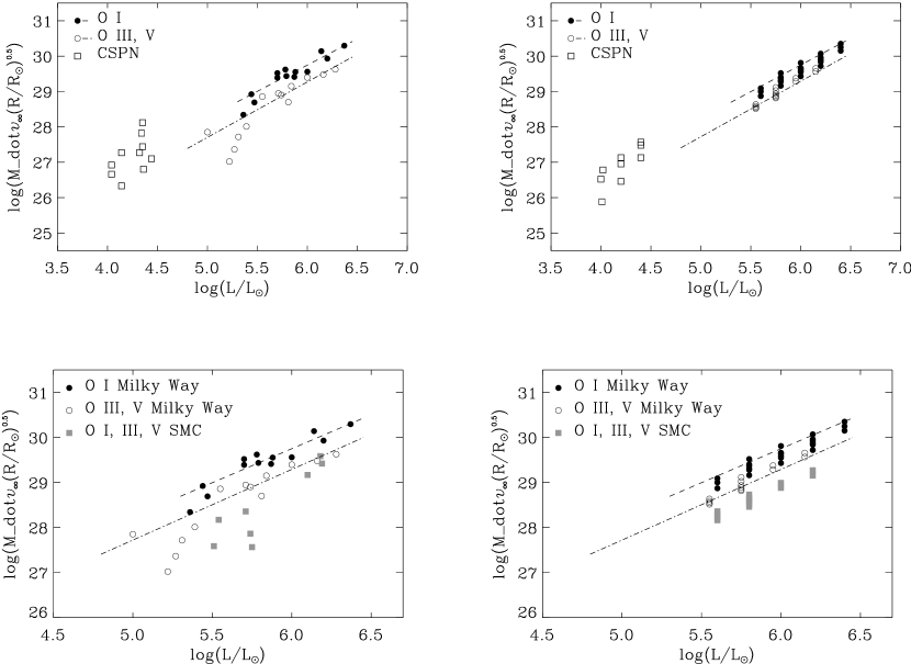
Figure 4: Top: Modified wind momenta of galactic O-stars and Central Stars of PN as a function of luminosity. Left: Observations (the dashed and dashed-dotted curves are linear regressions for the different O-star luminosity classes); right: model calculations as described in the text compared to the observed regression curves. Bottom: Modified wind momenta of O-stars in the galaxy and SMC as a function of luminosity. Left: Observations; right: calculations as described in the text. The linear regressions for galactic O-stars of the top figure are also shown.

depends mostly on stellar luminosity and much less on other stellar parameters. This prediction has been confirmed very convincingly by the empirical spectroscopic diagnostics of O-star winds. Fig. 4 shows the observed modified wind momenta of galactic O-stars and Central Stars of Planetary Nebulae (CSPN) as taken from Kudritzki and Puls (2000). Both the O-supergiants and O-giants and -dwarfs follow rather tight relationships, which when extrapolated towards lower luminosities coincide with the observed wind momenta of CSPN (for the two dwarfs falling off the relationship, see discussion in Puls et al. 1996).

Fig. 4 also shows the results of the model calculations using our new approach with the force multipliers given in Table 1. The models for O-stars have effective temperatures of 50000 and 40000 K, respectively. For the supergiants we have adopted gravities log g between 3.75 to 3.95 at 50000K and 3.35 to 3.50 at 40000K. Giants and dwarfs have larger gravities, 4.10 to 4.20 at 50000K and 3.7 to 4.0, respectively, at 40000K. These values coincide roughly with the stellar parameters observed. To calculate the winds of the CSPN the core-mass luminosity relationship for post-AGB has been adopted to estimate stellar masses and gravities at the corresponding luminosities. Solar metallicity was used for all the wind models of galactic objects.

The agreement with the regression curves resulting from the observations is satisfying though not perfect. The models for the supergiants produce slightly too weak winds and the opposite is the case for the dwarfs and giants. However, the general trend is reproduced very well. This indicates that our algorithm to calculate radiative line forces produces fmps of the right order of magnitude. In addition, the concept of variable fmps leads to a more pronounced difference between wind models close to the Eddington-limit and on the main sequence in better agreement with the observations.

In addition, Fig. 4 compares wind momenta of O-stars in the Galaxy and the metal poor SMC showing that winds are significantly weaker at lower metallicities (again from Kudritzki and Puls 2000). The calculations reproduce this trend, as is shown by Fig 4 as well. The stellar parameters used for the SMC calculations are identical to those for the Galaxy, except that Z = 0.2 Z_⊙ has been adopted for the metallicity following the results obtained by Haser et al. (1998) from the analysis of HST spectra of O-stars in the SMC. We have restricted the SMC calculations to dwarfs and giants because all but the most luminous object in Fig. 10a belong to these luminosity classes. As for the Milky Way there are a few (three) objects at lower luminosities, which fall off the relationship and the theory is not able to explain their wind momenta (but see Kudritzki and Puls, 2000, for discussion). In general, because of the small number of objects studied so far, the WLR in the SMC is not as well defined as in the Milky Way. More spectroscopic work is needed to improve the situation.

A comparison between calculated and observed terminal velocities of the stellar winds is another important test of the theory. For galactic O-stars this is carried out in Fig. 5, which displays terminal velocities as a function of photospheric escape velocities, since the theory predicts that both are correlated to first order. The result of the test is quite encouraging, although the observed terminal velocities are on the average somewhat higher than the calculated ones by 5 to 10 percent. Whether this small discrepancy reflects a deficiency of the theory or a systematic effect resulting from the determination of the observed escape probabilities, is an open question which is beyond the scope of this paper.

Metallicity does also affect the terminal velocities of stellar winds in a systematic way so that winds become slower with decreasing metal abundance, as investigations of O-stars in the Magellanic Clouds have revealed (refer to Kudritzki and Puls 2000, for references and a compilation of results). Fig. 5 shows that this effect is also reproduced by the theory.

6 Wind models for very massive stars at low metallicity

After the new concept to calculate stellar wind structures with variable force multipliers has been introduced and tested by comparing with the observed wind properties of O-stars in the Galaxy and the SMC, we are now ready for an application on very massive stars. The purpose of this first study is to provide an estimate about the strengths of stellar winds at very low metallicity for very massive hot stars in a mass range roughly between 100 to 300 M_⊙. We concentrate on an effective temperature range comparable to the hottest and most massive observed O-stars, i.e. 60000K to 40000K, which is only a mild extrapolation away from a stellar parameter regime, where the theory has been tested at galactic and SMC metallicity. We are fully aware of the fact that at the low metallicities used the zero age main sequences of stars in this mass range are shifted to higher effective temperatures ($\approx$ 75000K, see Baraffe et al. 2001) than accounted for in our calculations. However, at this stage we do not aim at a comprehensive description of stellar winds of metal poor very massive stars through all stages of their evolution. Instead, we restrict ourselves to a temperature regime, where the winds of massive stars at normal metallicity are well understood. We defer a more complete description connected with realistic evolutionary tracks to a second paper.

In a first step, following the discussion in section 2, we will investigate the strengths of low metallicity winds as a function from the distance to the Eddington limit. We will then define a simple schematic grid of stellar parameters, which will allow to investigate the systematic behavior of mass-loss rates, wind velocities, wind momenta and wind energies. We will use the full set of wind models calculated for this grid to provide simple analytical fit formulae for stellar wind properties as a function of stellar parameters and metallicity.

6.1 Low metallicity winds and the distance to the Eddington - Limit

In Section 2 we concluded from simple analytical considerations that line driven winds at very low metallicity can only be maintained if stars are close enough to the Eddington-limit so that the effective gravity becomes negative somewhere out in the wind. To investigate this effect by using the full stellar wind equations and a realistic line acceleration we have calculated sequences of models at constant luminosity and effective temperature but with the different stellar masses and, therefore, different distances to the Eddington-limit. The result is displayed in Fig. 6. The small and smooth dependence of the modified stellar wind momentum on $\Gamma$ for solar and SMC metallicity is well understood in terms of the discussion given by Puls et al. (1996). For constant luminosity the scaling relations of line driven winds predict

$$logD_{\rm mom}\propto(3/2-1/\alpha^{\prime})\cdot logM(1-\Gamma)\propto(3/2-1/\alpha^{\prime})\cdot log(1/\Gamma-1),$$ (53)

which means that the stellar wind momenta should decrease slightly with decreasing $\Gamma$, if $\alpha^{\prime}\leq 2/3$. The average force multiplier parameters of O-stars in the Galaxy and the Magellanic Clouds lead to values of $\alpha^{\prime}$ between 0.50 to 0.55, which explains the $\Gamma$-dependence of wind momenta in the corresponding range of metallicities. For Z/Z_⊙ = 0.01 the slope with $\Gamma$ becomes much stronger corresponding to an average $\alpha^{\prime}$ of the order of 0.4. It is, however, still possible to find wind solutions in the full range of $\Gamma$ appropriate for the luminosity adopted (note that $\Gamma$ = 0.4 corresponds to 119 M_⊙ at log L/L_⊙ = 6.26). For smaller metallicities the slope becomes even steeper and winds become very weak as soon as a certain threshold in $\Gamma$ is reached. For lower $\Gamma$, no wind solutions could be found, confirming qualitatively the analytical estimate of section 2.

6.2 Adopted stellar parameters for very massive objects

The goal of this paper is to investigate systematically the role of winds as function of metallicity and stellar parameters for hot stars in a mass range between 100 to 300 M_⊙. To do this consistently, i.e. by a combination of evolutionary tracks with stellar wind models is complicated because of the mutual dependence. For a given stellar mass, the evolution of a massive star, i.e. its location in the HRD depends strongly on metallicity but also on the strength of mass-loss. On the other hand, the properties of stellar winds depend also very strongly on the stellar parameters adopted and, of course, on metallicity. To disentangle this mutual dependence we proceed in a straightforward way. We define stellar parameters independent of metallicity for very simplified evolutionary sequences. In this way, we ignore the detailed effects of metallicity on the stellar evolution but we will be able to discuss its direct influence on stellar winds. Using the full information of wind models calculated for the grid of different stellar parameters and the different sets of metallicities we will then be able to provide fit formulae which can be used in conjunction with consistent evolutionary calculations in the future.

Our starting point is the paper by Schaller et al. (1992) which provides stellar models from 0.8 to 120 M_⊙ at solar and 1/20 solar metallicity. For our considerations we concentrate on their low metallicity models, which at their high mass end lead to a zero age main sequence mass-luminosity relationship of

$$log(L/L_{\odot})^{ZAMS}=6.095+1.53\cdot\{log(M/M_{\odot})-2\}$$ (54)

Evolving away from the ZAMS these objects gain roughly 0.2 dex in luminosity. Thus, we adopt for the more advanced evolutionary state in the temperature range of 60000 to 40000 K considered in this study

$$log(L/L_{\odot})=log(L/L_{\odot})^{ZAMS}+0.2$$ (55)

Eq. 54 and 55 can then be used to calculate radii and wind models at 40000, 50000 and 60000K effective temperature for the masses as indicated in Fig. 7. A comparison with models of very massive stars published in the literature (see, for instance, Bromm et al. 2001b, Baraffe et al. 2001) shows that this simple extrapolation is quite reliable.

6.3 Stellar wind properties

Table 2 gives a complete overview of the stellar wind properties for every model calculated and provides terminal velocity, mass-loss rate and modified wind momentum together with stellar parameters and metallicity. In the following we discuss the most important systematic trends using the models at T_eff = 50000K as an example.

Fig. 8 displays the modified stellar wind momentum as function of luminosity for models at different metallicity. The simplified theory of radiation driven winds with depth independent and luminosity independent force multiplier parameters predicts a simple relationship of the form

$$logD_{\rm mom}\propto 1/\alpha^{\prime}\cdot logL+(1-\alpha^{\prime})/\alpha^{\prime}\cdot(Z/Z_{\odot}),$$ (56)

(Kudritzki et al. 1989, Puls et al. 1996, Kudritzki and Puls 2000). Fig. 8 confirms that, in principle, such a relationship continues to exist for the more elaborated force multiplier approach developed in this paper, however the effective value of $\alpha^{\prime}$ depends now on both, luminosity and metallicity. In particular, it decreases very significantly with metallicity (see also discussion in section 6.1) so that the dependence of wind momentum on luminosity becomes much steeper with decreasing metallicity. This trend becomes also obvious in Fig. 9, where the stellar wind properties are plotted as function of metallicity. Mass-loss, modified wind momentum and wind energy decrease stronger than a simple power law with metallicities beyond $Z/Z_{\odot}$ = 0.01.

In the same framework of simplified wind theory with constant force multipliers the terminal velocity of the stellar wind is related to the escape velocity from the stellar surface via the proportionality (Kudritzki and Puls 2000)

$$v_{\infty}/v_{esc}\propto\alpha/(1-\alpha)\cdot exp(-2\delta).$$ (57)

From Fig. 9 we have learned that the effective value of $\alpha^{\prime}$ and, thus, also $\alpha$ is decreasing at low metallicities. According to Eq. 57 we, therefore, expect smaller ratios of $v_{\infty}/v_{esc}$ at the low metallicity end as the result of our calculations, which is confirmed by Fig. 9. In addition, we find that the ratio does also depend on luminosity and becomes smaller with decreasing luminosity.

6.4 An analytical fit of mass-loss rates to stellar parameters and metallicity

Stellar evolution calculations for very massive stars need to include the effects of mass-loss as soon as the mass-loss rates are high enough to reduce the total stellar mass significantly during the different phases of stellar evolution. While in the range of solar and Magellanic Cloud metallicities the standard formulae resulting from the theory of line driven winds or fits to the observed data are usually applied, nothing comparable is available for the stellar parameter and metallicity domain investigated here. We have, therefore, developed a simple analytical fit-formula to our numerical results, which provides mass-loss rates of line driven winds. It can easily be combined with stellar evolution calculations or used to estimate the energy and momentum input of very massive low metallicity stars to the interstellar medium.

$$log\dot{M}=Q([Z])=q_{1}([Z]-[Z]_{min})^{0.5}+Q_{min},\qquad\qquad q_{1}=(Q_{0}-Q_{min})(-[Z]_{min})^{-0.5}.$$ (58)

[Z] is defined as

$$[Z]=log(Z/Z_{\odot})$$ (59)

$[Z]_{min},Q_{min},Q_{0}$ depend on the luminosity through a simple polynomial formula

$$y=a_{0}+a_{1}\tilde{L}+a_{2}\tilde{L}^{2},\qquad\qquad\tilde{L}=log(L/L_{\odot})-6.0.$$ (60)

The coefficients are $a_{0},a_{1},a_{2}$ for the fits of y=$[Z]_{min},Q_{min},Q_{0}$ are given in Table  3.

6.5 Decoupling of radiatively accelerated ions at low metallicity

The key process of line driven winds is the transfer of radiative momentum absorbed in spectral line transitions of metal ions to the bulk mass of ionized hydrogen and helium, which because of the lack of enough strong line transitions is not much driven directly by radiation. For the strong and relatively dense winds of O-stars at solar metallicity the transfer mechanism is provided by Coulomb collisions, which keep the metal and the hydrogen/helium ions tightly coupled together, as has been shown by Castor et al. (1976). However, for weak winds with low mass-loss rates and correspondingly low densities the lower collision rates can lead to a decoupling of the ions from the bulk plasma and produce a “ion runaway” reducing mass-loss rate and wind momentum significantly (Springmann and Pauldrach 1992, Babel 1995, Porter and Drew 1995, and Porter and Skouza 1999). The effect of a runaway was put into question recently by Krticka and Kubat (2000), Krticka and Kubat (2001), who were the first to derive complete quantitative solutions for two-component (ions and passive plasma) steady state line driven winds. They found that in the limit of low density winds both the ions and the passive plasma adopt a solution of lower acceleration and avoid the runaway. This very interesting result was then challenged very recently by Owocki and Puls (2002), who carried out a time-dependent, linearized stability analysis of the two-component solutions and found that a runaway is very likely to happen in the wind flow, before the wind adopts the steady, slow-acceleration solutions. Thus, the situation in the low density limit of weak winds remains unclear at this point but there is the clear potential that normal single-fluid solutions might become unrealistic in this limit.

At the extremely low metallicities considered in this investigation the single-fluid solutions might have crossed over into a parameter domain, where their validity has become questionable, because the rate of Coulomb collisons has dropped significantly because of extremely low mass-loss rates and the very low abundance of ions. We have, therefore, used equation 16b (corrected for a numerical mistake in their treatment of the Coulomb Logarithm) of Springmann and Pauldrach and equation 22 of Owocki and Puls to check, which of our models are in a critical parameter domain with regard to a possible runaway.

For $Z/Z_{\odot}$ = 0.0001 the models with $logL/L_{\odot}$ = 6.91 might suffer from a runaway, but only at velocities of the order of one half to one third the terminal velocity and certainly larger than the critical velocity, thus probably still little affected by two-component effects. The same is true for some models with $Z/Z_{\odot}$ = 0.001 and $logL/L_{\odot}\leq$ 6.42. A more detailed investigation will be needed for these models, but we conclude that in general the winds calculated in our model grid are only marginally affected by ion decoupling.

7 Ionizing fluxes and stellar spectra

With the stellar wind structures and parameters specified in the previous sections we can now calculate detailed atmospheric models together with stellar energy distributions and synthetic spectra for all the models in Table 2 . For this purpose we used the approach of ”Unified Model Atmospheres” as developed at Munich University Observatory over the last 15 years. These model atmospheres are in NLTE, radiative equilibrium, spherically extended and include the effects of stellar winds (see Gabler et al. 1989, for the original introduction of the concept and Pauldrach et al. 1994, for a first version including metal lines). The most recent step of this development by Pauldrach et al. (2001) accounts for more than 4 millions of metal lines in NLTE originating from more than 150 metal ions. Detailed atomic models with accurate atomic data are set up for every ion, for which the equations of statistical equilibrium are solved consistently and simultaneously with the radiative transfer in each line and ionization transition in a highly iterative algorithm. Multi-line absorption is included in the radiative transfer and in the radiative equilibrium, which means that the effects of line-blanketing and -blocking are fully taken into account. After convergence spectra and energy distributions are calculated including all the spectral lines. The code is thus ideally suited to demonstrate the transition from solar to very low metallicity. In addition, despite the complexity of the atomic models and the radiative transfer algorithms the code is extremely fast and produces a converged model on a laptop or PC in a few hours. It is public available and can be downloaded from the Munich University Observatory website (http://www.usm.uni-muenchen.de/people/adi/adi.html). For details we refer the reader to the original publication.

Fig. 10 gives an example of the effects of metallicity on the EUV and FUV spectral energy distribution. We have selected two models at $T_{eff}$ = 60000K at two different luminosities, log $L/L_{\odot}$ = 6.57 and 6.91, respectively. Longward of 228A, in the H, HeI, OII, NeII, CIII ionizing continuum, the influence of metal line opacity is very similar at both luminosities. Increased metallicity decreases the emergent flux within the metal lines because of enhanced line blocking but increases the flux emitted in the continuum windows with reduced line opacity because of the back-warming effects of line-blanketing. The balance between the different influence of blocking and blanketing will, therefore, determine how the ionizing properties of these stars are affected by metallicity (see below).

Shortward of 228A, in the HeII ionizing continuum, metallicity has a dramatic influence on the size of the HeII absorption edge and, thus, on the ionizing flux. However, this influence is less related to the effects of line-blanketing and -blocking rather than to the strengths of the stellar winds correlated with metallicity (see Gabler et al. 1989, Gabler et al. 1991, Gabler et al. 1992 for a detailed explanation).

Fig. 11 summarizes the effects of metallicity on the ionizing properties of very massive stars. For three effective temperatures and two luminosities we show the number of emerging ionizing photons per stellar surface element and unit time as a function of metallicity. To characterize the wavelength dependence of the ionizing radiation we display the number of photons being able to ionize H (ionization edge at 911A), HeI (504A), OII (353A), NeIII (303A), CIII (259A) and HeII (228A). The dependence on metallicity of these photon numbers varies significantly with the ionization edge approaching the limit of HeII ionization. While the number of H photons remains almost constant and the effects of metal line-blocking and -blanketing balance out over the relatively wide spectral range from the hydrogen to the HeII absorption edge, the number of CIII photons decreases strongly with increasing metallicity, because line blocking dominates the remaining wavelength interval towards the HeII absorption edge.

The HeII ionizing photons reflect a more complex behavior as discussed above. At solar metallicity winds can become highly optically thick in the HeII continuum and then the number of ionizing photons drops dramatically. As soon as the winds become weak enough, the velocity field induced ground-state de-population (Gabler et al., 1989) sets in and increases the photon number substantially. Then, with decreasing metallicity the winds become weaker, which reduces the influence of the de-population effect. Since the wind strengths depend strongly on stellar luminosity, the detailed metallicity dependence of the HeII photons varies with luminosity. Fig. 12 gives examples for $T_{eff}$ = 60000K and 50000K, respectively. Thus, to predict the ionizing flux in the HeII continuum appropriately for a very massive star at a given metallicity requires a calculation of the wind parameters first.

The luminosity dependence of the ionizing photons for hydrogen and neutral helium turns out to be very weak. To a very good approximation the numbers displayed in Fig. 11 are representative. The luminosity effect for the OII, NeII photons is somewhat larger but still small. The largest effects are found for the CIII photons as displayed in Fig. 12.

It is also interesting to calculate synthetic FUV and UV spectra as a function of metallicity. As we know well from IUE, HST, ORFEUS and FUSE observations of massive stars in the Galaxy and the Large and Small Magellanic Cloud, the observed spectra in this spectral range are heavily blended by a dense forest of slightly wind affected pseudo-photospheric metal absorption lines superimposed by broad P Cygni and emission line profiles of strong lines formed in the entire wind. Model atmosphere synthetic spectra are able to reproduce the spectra nicely (Haser et al. 1998, de Koter et al. 1988, Fullerton et al. 2000, Pauldrach et al. 2001), demonstrating the reliability of the model atmosphere approach. The interesting question to investigate is to find the metallicity range, where the UV stellar wind features and the photospheric metal lines absorption lines start to disappear. Fig. 13 gives an overview for log L/L_⊙ = 6.91, where the winds are relatively strong. The stellar wind lines (NV $\lambda$ 1240, OV $\lambda$ 1371, CIV $\lambda$ 1550, HeII $\lambda$ 1640) remain clearly visible down to Z/Z_⊙ = 10^-2, where the absorption forest has already started to disappear. For lower metallicity, the stellar wind character of these lines disappears, but they are still detectable as photospheric absorption or emission lines. This means that for starbursting galaxies at very high redshift and possibly very low metallicities, as eventually observable with NGST in the IR, there is still diagnostic information available to estimate chemical abundances and further properties such as the Initial Mass Function and the star formation rate of the integrated stellar population.

8 Discussion and future work

With our new approach to describe line driven stellar winds at extremely low metallicity we were able to make first predictions of stellar wind properties, ionizing fluxes and synthetic spectra of a possible population of very massive stars in this range of metallicity $Z/Z_{\odot}$. We have demonstrated that the normal scaling laws, which predict stellar-mass loss rates and wind momenta to decrease as a power law with $Z/Z_{\odot}$ break down at a certain threshold and we have replaced the power-law by a different fit-formula. We were able to disentangle the effects of line-blocking and line-blanketing on the ionizing fluxes and found that while the number of photons able to ionize hydrogen and neutral helium is barely affected by metallicity (and stellar luminosity), there is a significant increase of the photons which can ionize OII, NeII, CIII, with decreasing metallicity, the effect being strongest for those ionic species with ionization edges closest to the HeII absorption edge. The HeII ionizing photons are very strongly affected by metallicity (and luminosity) through the strengths of stellar winds. We also calculated synthetic spectra and were able to present for the first time predictions of UV spectra of very massive stars at extremely low metallicities. From these calculations we learned that the presence of stellar winds leads to observable broad spectral line features, which might be used for spectral diagnostics, should such an extreme stellar population be detected at high redshift.

We find these first steps very encouraging to proceed with our calculations towards a number of improvements and extensions in the future. So far, our stellar parameters have been chosen from simple scaling relations and not from consistent stellar interior and evolution calculations. While this was certainly sufficient at the beginning to find out what the basic effects are, we need to remove this deficiency in a next step to become more quantitative. We also have to increase the range of effective temperatures, since the zero age main sequences of very massive stars are shifted beyond 60000K for metallicities as low as in this paper (Bromm et al. 2001b, Tumlinson and Shull 2000, Chiosi et al. 2000, Baraffe et al. 2001). In this way, we will be able to make improved predictions about the influence of stellar winds on the evolution of very massive stars and on the evolution of galaxies through deposition of matter, radiation, momentum and energy. These improved calculations should also take into account the effects of changes in the chemical abundance pattern of metals. So far, we have adopted relative abundances as in the solar system and have only scaled the total metallicity. However, it is very likely that an early generation of very massive stars will have an abundance pattern substantially different from the sun, in particular with regard to the ratio of $\alpha$ to iron group elements. As has been shown by Puls et al. (2000) and Vink et al. (2001) in the case of normal O-stars, this can have a significant influence on the stellar wind properties.

Acknowledgments

It is a pleasure to thank my former Munich University Observatory colleagues Adi Pauldrach, Joachim Puls and Uwe Springmann for their active support during the time, when this work was started. Volker Bromm and Avi Loeb directed my attention to the important role of very massive stars in the early universe and motivated much of the work done here. Special thanks go to Fabio Bresolin and Roberto Mendez for careful reading of the manuscript and critical remarks. The detailed and very constructive comments of the referee are gratefully acknowledged.

Appendix A Appendix. The functions $D_{\alpha}$ and $\Delta v_{reg}$

Eqs. 42, 43 and 45 contain the function $D_{\alpha}$ which follows from the derivative of the first term of Eq. 31 with respect to y

$$D_{\alpha}=D_{0}+D_{1}-D_{2}$$ (A1)

with

$$D_{0}=1+\frac{{\hbox{$\alpha_{0}\alpha_{1}$}}}{{\hbox{$\alpha$}}}log(t),\qquad\qquad D_{2}=\frac{{\hbox{$\gamma$}}}{{\hbox{$\alpha$}}}log(\hat{n}),$$ (A2)

$$D_{1}=\frac{{\hbox{$1$}}}{{\hbox{$\alpha$}}}\{\frac{{\hbox{$\alpha_{0}\alpha_{1}$}}}{{\hbox{$\alpha+1$}}}\frac{{\hbox{$1$}}}{{\hbox{$ln(10)$}}}-\frac{{\hbox{$h$}}}{{\hbox{$1-h$}}}+(\alpha+1)\frac{{\hbox{$(1-\lambda)^{\alpha+1}$}}}{{\hbox{$1-(1-\lambda)^{\alpha+1}$}}}H\},$$ (A3)

and

$$H=u^{2}h+\frac{{\hbox{$\alpha_{0}\alpha_{1}$}}}{{\hbox{$\alpha+1$}}}(1-\lambda)log(1-\lambda).$$ (A4)

Note that with constant $\alpha$ (i.e. $\alpha_{1}=0$) $D_{\alpha}$ simplifies to

$$D_{\alpha}=D_{\alpha}^{0},\qquad\qquad D_{\alpha}^{0}=1+\frac{{\hbox{$1$}}}{{\hbox{$\alpha$}}}\{(\alpha+1)\frac{{\hbox{$(1-\lambda)^{\alpha+1}$}}}{{\hbox{$1-(1-\lambda)^{\alpha+1}$}}}u^{2}h-\frac{{\hbox{$h$}}}{{\hbox{$1-h$}}}\}$$ (A5)

describing the influence of the finite cone angle correction factor on the derivative with respect to y (see Pauldrach et al. (1986)). Neglecting the finite cone angle correction factor leads to $D_{\alpha}^{0}=1$.

The function $\Delta v^{2}_{reg}$ in Eq. 44 is given by

$$\Delta v^{2}_{reg}=-\frac{{\hbox{$1$}}}{{\hbox{$2a_{0}$}}}\{a_{1}+(a_{1}^{2}-4a_{0}a_{2})^{0.5}\}$$ (A6)

where the coefficients $a_{0,1,2}$ are defined as

$$a_{0}=\frac{{\hbox{$a$}}}{{\hbox{$1-\alpha_{eff}$}}}\frac{{\hbox{$2$}}}{{\hbox{$u$}}}D_{u}-\frac{{\hbox{$v_{s}^{2}$}}}{{\hbox{$v_{esc}^{2}$}}}\frac{{\hbox{$4$}}}{{\hbox{$u^{2}$}}},$$ (A7)

$$a_{1}=-\alpha_{eff}\{\frac{{\hbox{$a$}}}{{\hbox{$1-\alpha_{eff}$}}}\}^{2}v_{esc}^{2}D_{v},\qquad\qquad a_{2}=(\alpha_{eff})^{2}\{\frac{{\hbox{$a$}}}{{\hbox{$1-\alpha_{eff}$}}}\}^{2}v_{esc}^{2}v_{s}^{2}.$$ (A8)

The functions $D_{u}$ and $D_{v}$ are connected with the partial derivatives of the function f with respect to u and v

$$\frac{{\hbox{$1$}}}{{\hbox{$f$}}}\frac{{\hbox{$\partial f$}}}{{\hbox{$\partial u$}}}=\frac{{\hbox{$2$}}}{{\hbox{$u$}}}D_{u},\qquad\qquad\frac{{\hbox{$1$}}}{{\hbox{$f$}}}\frac{{\hbox{$\partial f$}}}{{\hbox{$\partial v^{2}$}}}=\frac{{\hbox{$1$}}}{{\hbox{$v^{2}$}}}D_{v}$$ (A9)

and calculated by

$$D_{u}=\delta D_{W}D_{\delta}-\frac{{\hbox{$1-h/2$}}}{{\hbox{$1-h$}}}D_{\lambda},\qquad\qquad D_{v}=\frac{{\hbox{$h$}}}{{\hbox{$1-h$}}}D_{\lambda}-\frac{{\hbox{$\delta$}}}{{\hbox{$2$}}}D_{\delta},$$ (A10)

where

$$D_{\lambda}=1-(\alpha+1)\lambda\frac{{\hbox{$(1-\lambda)^{\alpha}$}}}{{\hbox{$1-(1-\lambda)^{\alpha+1}$}}},$$ (A11)

and

$$D_{\delta}=1+\frac{{\hbox{$\delta_{0}\delta_{1}$}}}{{\hbox{$\delta$}}}log(\hat{n}),\qquad\qquad D_{W}=1-\frac{{\hbox{$1$}}}{{\hbox{$4$}}}\frac{{\hbox{$u^{2}$}}}{{\hbox{$W(u)(1-u^{2})^{0.5}$}}}.$$ (A12)

Table 1: New force multiplier parameters

Teff	Z/Z⊙	$\hat{k}$	$\alpha_{o}$	$\alpha_{1}$	$\delta_{o}$	$\delta_{1}$	$\gamma$
40000	1.0	0.074	0.697	0.018	0.199	0.037	0.032
	0.2	0.054	0.715	0.029	0.192	-0.046	0.030
	0.001	0.010	0.778	0.061	0.018	-0.726	-0.028
	0.0001	0.008	0.488	-0.013	-0.063	0.457	-0.067
50000	1.0	0.084	0.695	0.021	0.197	-0.134	-0.007
	0.2	0.041	0.798	0.042	0.233	-0.019	0.019
	0.01	0.031	0.728	0.054	0.068	0.185	-0.024
	0.001	0.018	0.673	0.050	-0.026	0.556	-0.073
	0.0001	0.008	0.548	-0.003	-0.084	0.462	-0.105
60000	1.0	0.028	0.668	-0.008	0.266	0.249	-0.065
	0.2	0.023	0.743	0.027	0.223	0.198	0.045
	0.01	0.026	0.722	0.062	0.163	0.096	0.004
	0.001	0.016	0.662	0.062	0.036	0.714	-0.064
	0.0001	0.004	0.773	0.061	-0.133	0.045	-0.154

Table 2: Stellar parameter and stellar wind properties

log L/L⊙	Teff	log g	R/R⊙	Z/Z⊙	v∞	$\dot{M}$	log Dmom
7.03	60000.	3.95	30.38	1.0	1043.4	483.6	31.24
				0.2	1176.4	138.5	30.75
				0.01	1251.5	59.9	30.41
				0.001	890.9	19.5	29.78
				0.0001	711.7	2.2	28.73
	50000.	3.63	43.76	1.0	1211.5	591.4	31.47
				0.2	1372.1	263.4	31.18
				0.01	1182.8	63.9	30.50
				0.001	911.2	17.5	29.82
				0.0001	612.7	2.4	28.80
	40000.	3.25	68.32	1.0	943.0	528.2	31.41
				0.2	971.7	226.9	31.06
				0.001	730.9	10.0	29.58
				0.0001	424.3	1.2	28.45
6.91	60000.	3.99	26.24	1.0	1215.0	116.8	30.66
				0.2	1399.2	41.7	30.27
				0.01	1280.6	26.3	30.04
				0.001	958.8	4.8	29.17
				0.0001	495.9	0.2	27.59
	50000.	3.68	38.06	1.0	1830.9	219.5	31.19
				0.2	1731.2	109.4	30.86
				0.01	1307.2	27.9	30.15
				0.001	1035.4	5.8	29.37
				0.0001	555.9	0.3	27.92
	40000.	3.28	59.49	1.0	1176.1	211.1	31.08
				0.2	1248.6	92.6	30.75
				0.001	879.4	3.2	29.14
				0.0001	425.3	0.1	27.46
6.76	60000.	4.04	22.29	1.0	1272.9	31.9	30.08
				0.2	1622.5	16.0	29.89
				0.01	1405.3	8.7	29.56
				0.001	939.9	0.9	28.44
	50000.	3.73	32.10	1.0	2205.2	100.6	30.90
				0.2	1839.5	55.0	30.56
				0.01	1443.3	11.4	29.77
				0.001	1029.8	1.9	28.85
	40000.	3.34	50.12	1.0	1476.5	79.7	30.72
				0.2	1423.6	40.9	30.41
				0.001	926.7	1.0	28.64
6.57	60000.	4.11	17.78	1.0	1799.7	9.2	29.64
				0.2	2147.5	5.3	29.48
				0.01	1507.4	2.4	28.99
				0.001	745.4	0.07	27.14
	50000.	3.79	25.74	1.0	2270.1	48.3	30.54
				0.2	1947.6	24.3	30.18
				0.01	1518.0	4.1	29.30
				0.001	923.0	0.4	28.14
	40000.	3.41	40.18	1.0	1545.0	36.3	30.35
				0.2	1641.5	16.6	30.04
				0.001	900.2	0.2	28.01
6.42	60000.	4.16	15.07	1.0	2426.5	4.3	29.41
				0.2	2469.1	2.7	29.21
				0.01	1535.8	1.0	28.58
	50000.	3.85	21.71	1.0	2279.4	29.0	30.29
				0.2	2021.0	13.3	29.90
				0.01	1525.7	2.0	28.96
				0.001	771.2	0.13	27.47
	40000.	3.46	33.93	1.0	1675.1	19.7	30.08
				0.2	1746.5	9.1	29.77
				0.001	846.9	0.10	27.51
6.30	60000.	4.21	13.11	1.0	2939.8	2.6	29.24
				0.2	2693.1	1.6	29.00
				0.01	1539.4	0.51	28.25
	50000.	3.89	18.88	1.0	2301.6	18.9	30.07
				0.2	2056.2	8.4	29.67
				0.01	1513.5	1.1	28.68
	40000.	3.50	29.51	1.0	1767.5	12.2	29.87
				0.2	1809.7	5.7	29.55
				0.001	795.4	0.04	27.07

Table 3: Fit parameters for mass-loss formula

y	Teff	$a_{0}$	$a_{1}$	$a_{2}$
$[Z]_{min}$	60000.	-3.40	-0.40	-0.65
	50000.	-3.85	-0.05	-0.60
	40000.	-4.45	0.35	-0.80
$Q_{min}$	60000.	-8.00	-1.20	2.15
	50000.	-10.35	3.25	0.00
	40000.	-11.75	3.65	0.00
$Q_{0}$	60000.	-5.99	1.00	1.50
	50000.	-4.85	0.50	1.00
	40000.	-5.20	0.93	0.85

Figure 1: Top: Line force multiplier ${\it M(t)}$ as a function of optical depth parameter t for T_eff = 50000K and metallicities Z = 1.0, 0.01 and 0.001 Z_⊙. The solid curves correspond to a density log n${}_{e}/W$ = 10.0, for the dashed curves the density is 0.25 dex smaller. Middle: Logarithmic derivative $\alpha$ of the line force multipliers in the top panel as defined in Eq. 20. Bottom: Logarithmic derivative $\delta$ of the line force multipliers in Fig. 1 as defined in Eq. 24. Note that both line force parameters, $\alpha$ and $\delta$, vary strongly as function of optical depth for metallicites smaller than solar.

Figure 2: Isocontours of line force parameters $\alpha$ (top panel) and $\delta$ (middle panel) in the (log n${}_{e}/W$, log t)-plane. The bottom panel shows the isocontours of the HeII contribution to the line force (in percent). All calculations are for T_eff = 50000K. Left panels: Z = 10^-2 Z_⊙; right panels: Z = 10^-4 Z_⊙. For discussion see text.

Figure 3: Top: Isocontours of the difference between log ${\it M(t)}$ and log ${\it M(t)}_{fit}$, where the latter is calculated with constant values of $\alpha$ and $\delta$ according to Eq. 15. Bottom: The same as top, but now with log ${\it M(t)}_{fit}$ calculated according to Eq. 25. Left: Z = 10^-2 Z_⊙; right: Z = 10^-4 Z_⊙.

Figure 5: Top: Terminal velocity of galactic O-stars versus photospheric escape velocity. Open circles represent observations taken from Lamers et al.(1995). Solid circles corresponds to the calculations as described in the text. Bottom: The influence of metallicity on the computations of terminal velocities for O main sequence stars. Open circles correspond to the calculations for galactic metallicity. Solid circles represent calculations for Z = 0.2 Z_⊙.

Figure 6: Modified stellar wind momenta as a function of $\Gamma$, the ratio of electron scattering radiative acceleration to gravitational acceleration. All models have been calculated for T_eff = 50000 K and log L/L_⊙ = 6.26. The different sequences are labelled by the value of the metallicity Z/Z_⊙ adopted.

Figure 7: The HRD of the simplified stellar models adopted for the stellar wind calculations. The tracks are labelled by the stellar mass in solar units. Luminosities and effective temperatures of the wind models calculated for this study are given by filled circles.

Figure 8: Modified stellar wind momentum calculated as a function of stellar luminosity for models of different metallicity with Z/Z_⊙ = 1.0 (squares), 0.2 (triangles), 10^-2 (plus signs), 10^-3 (open circles) and 10^-4 (solid circles).

Figure 9: Stellar wind properties as a function of metallicity for models of different luminosity with log L/L_⊙ = 7.03 (solid circles), 6.91 (open circles), 6.76 (plus signs), 6.57 (asterisks), 6.42 (triangles), 6.30 (squares). Upper left: mass-loss rates, upper right: modified stellar wind momentum, lower left: wind energy, lower right: terminal velocity in units of photospheric escape velocity.

Figure 10: Logarithm of emergent EUV/FUV Eddington flux H_ν as a function of wavelength for models with T_eff = 60000K and two metallicities, Z/Z_⊙ = 1.0 (dotted) and 10^-4 (solid). Upper panel: log L/L_⊙ = 6.91, lower panel: log L/L_⊙ = 6.57. Note the dramatic differences in the HeII continuum shortward of 227 A.

Figure 11: Logarithm of the emitted number of ionizing photons as a function of stellar metallicity (see text). Left: log L/L_⊙ = 6.42; right: log L/L_⊙ = 7.03. Top panels: T_eff = 40000K; middle panels: T_eff = 50000K; bottom panels: T_eff = 60000K.

Figure 12: Logarithm of the emitted number of ionizing photons as a function of stellar metallicity (see text). Upper left panel: HeII-photons at T_eff = 50000K, log L/L_⊙ = 6.76 (squares), 6.91 (circles), 7.03 (solid circles). Upper right panel: HeII-photons at T_eff = 60000K, log L/L_⊙ = 6.57 (squares), 6.91 (circles), 7.03 (solid circles). Lower panels: CIII-photons at T_eff = 40000K (left) and 50000K (right) and luminosities log L/L_⊙ = 6.57 (squares), 6.91 (circles), 7.03 (solid circles).

Figure 13: Continuum rectified UV-spectra longward of Lyman-alpha for models with log L/L_⊙ = 6.91 and T_eff = 50000K (top panel) and 60000K (bottom panel). Each panel displays three metallicities, Z/Z_⊙ = 0.2 (top), 10^-2 (middle), 10^-4 (bottom). The strongest line features, which remain present at the lowest metallicity, are NV $\lambda$ 1250, OV $\lambda$ 1371A, CIV $\lambda$ 1550 and HeII $\lambda$ 1640A.

References

- Abbott (1982) Abbott D.C., 1982, ApJ, 259, 282
- Abel et al. (2000) Abel, T, Bryan, G.L., Norman, M.L., 2000, ApJ, 540, 39
- Abel et al. (2002) Abel, T, Bryan, G.L., Norman, M.L., 2002, Science, 295, 93
- Babel (1995) Babel, J., 1995, A&A, 301, 823
- Baraffe et al. (2001) Baraffe, I., Heger, A., Woosley, S.E., 2001, ApJ, 550, 890
- Becker et al. (2001) Becker, R.H. et al., 2001, AJ, 122, 2850
- Bromm et al. (1999) Bromm, V., Coppi, P.S., Larson, R.B., 1999, ApJ, 527, L5
- Bromm et al. (2001a) Bromm, V., Ferrara, A., Coppi, P.S., Larson, R.B., 2001a, MNRAS, 328, 969
- Bromm et al. (2001b) Bromm, V., Kudritzki, R.P., Loeb, A., 2001b, ApJ, 552, 464
- Bromm et al. (2002a) Bromm, V., Coppi, P.S., Larson, R.B., 2002a, ApJ, 540, 687
- Bromm et al. (2002b) Bromm, V., Loeb, A., 2002b, submitted (astro-ph/0201400)
- Castor et al. (1975) Castor J.I., Abbott D.C., Klein R.I., 1975, ApJ, 195, 157
- Castor et al. (1976) Castor J.I., Abbott D.C., Klein R.I., 1976, Physique des Mouvements dans les Atmospheres Stellaires, R. Cayrel and M. Steinberg, eds., CNRS, Paris, 363
- Carr et al. (1984) Carr, B.J., Bond, J.R., Arnett, W.D., 1984, ApJ, 277, 445
- Ciardi et al. (2000) Ciardi, B., Loeb, A., 2000, ApJ, 540, 687
- Chiosi et al. (2000) Chiosi, C., 2000, Proc. ESO Astrophysics Symposium “The First Stars”, Springer, eds. A. Weiss, T. Abel, V. Hill, page 95
- Couchman et al. (1986) Couchman, H.M.P., Rees, M.J., 1986, MNRAS, 221, 53
- de Koter et al. (1988) de Koter, A., Heap, S.R., Hubeny, I., 1998, ApJ, 509, 879
- Djorgovski et al. (2001a) Djorgovski, S.G., Castro, S., Stern, D., Mahabal, A.A., 2001a, ApJ, 560, L5
- Djorgovski et al. (2001b) Djorgovski, S.G. et al., 2001b, in press (astro-ph/0107535)
- Fan et al. (2000) Fan, X. et al., 2000, AJ, 120, 1167
- Fan et al. (2002) Fan, X. et al., 2002, in press (astro-ph/0111184)
- Fullerton et al. (2000) Fullerton, A. W., Crowther, P.A., de Marco, O. et al., 2000, ApJ, 538, L43
- Gabler et al. (1989) Gabler R., Gabler A., Kudritzki R.P., Pauldrach A.W.A., Puls J., 1989, A&A, 226, 162
- Gabler et al. (1991) Gabler R., Kudritzki R.P., Méndez R.H., 1991, A&A, 245, 587
- Gabler et al. (1992) Gabler R., Gabler A., Kudritzki R.P., Méndez R.H., 1992, A&A, 265, 656
- Gayley (1995) Gayley K, 1995, ApJ, 454, 410
- Haser et al. (1998) Haser, S.M., Pauldrach, A.W.A., Lennon, D.J., Kudritzki, R.P. et al., 1998, A&A, 330, 285
- Haiman et al. (1997) Haiman, Z., Loeb, A., 1997, ApJ, 483, 21
- Hu et al. (2002) Hu, E.M., Cowie, L.L., McMahon, R.J., Capak, P., Iwamuro, F., Kneib, J.P., Maihara, T., Motohara, K., 2002, ApJ, in press
- Krticka and Kubat (2000) Krticka, J., Kubat, J., 2000, A&A, 359, 983
- Krticka and Kubat (2001) Krticka, J., Kubat, J., 2001, A&A, 369, 222
- Kudritzki (1988) Kudritzki, R.P., 1988, In: Y. Chmielewski and T. Lanz (eds.), 18th Advanced Course of the Swss Society of Astrophysics and Astronomy (Saas-Fee Courses) “Radiation in Moving Gaseous Media”, pages 1 - 192
- Kudritzki (1998) Kudritzki R.P., 1998, In: Aparicio A., Herrero A., Sánchez F. (eds.) VIII Canary Islands Winter School of Astrophysics on Stellar Astrophysics for the Local Group, Cambridge University Press, 149
- Kudritzki et al. (1987) Kudritzki R.P., Pauldrach A.W.A., Puls J., 1987, A&A, 173, 293
- Kudritzki et al. (1989) Kudritzki R.P., Pauldrach A.W.A., Puls J., et al., 1989, A&A, 219, 205
- Kudritzki et al. (1998) Kudritzki R.P., Springmann U., Puls J., et al., 1998, ASP Conf. Series 131, 299
- Kudritzki and Puls (2000) Kudritzki R.P., Puls J., 2000, Annual Review of Astronomy and Astrophysics 38, 613
- Kulkarni et al. (2000) Kulkarni, S.R., et al., 2000, SPIE Proc. 4005, 9
- Lamb et al. (2000) Lamb, D.Q., Reichart, D.E., 2000, ApJ, 536, 1
- Leitherer et al. (1992) Leitherer C., Robert C., Drissen L., 1992, ApJ, 401, 596
- Leitherer et al. (2001) Leitherer C., Leao J.R.S., Heckman T.M., Lennon D.J., Pettini M., Robert C., 2001, ApJ, 550, 724
- Lucy and Abbott (1993) Lucy L.B., Abbott D.C., 1993. ApJ, 405, 738
- Malhotra and Rhoads (2002) Malhotra, S., Rhoads, J.E., 2002, submitted (astro-ph/0111126)
- Mac Fayden et al. (2001) MacFayden, A.I., Woosley, S.E., Heger, A., 2001, ApJ, 550, 410
- Najarro et al. (1996) Najarro F., Kudritzki R.P., Cassinelli J.P., Stahl O., Hillier D.J., 1996, A&A, 306, 892
- Nakamura and Umemura (2001) Nakamura, F., Umemura, M., 2001, ApJ, 548, 19
- Owocki et al. (1988) Owocki, S.P., Castor, J.I., Rybicki, G.B., 1988, ApJ, 335, 914
- Owocki and Puls (2002) Owocki, S.P., Puls, J., 2002, ApJ,, in press
- Pauldrach et al. (1986) Pauldrach A.W.A., Puls J., Kudritzki R.P., 1986, A&A, 164, 86
- Pauldrach et al. (1994) Pauldrach A.W.A., Kudritzki R.P., Puls J. et al., 1994, A&A, 283, 525
- Pauldrach et al. (1998) Pauldrach A.W.A., Lennon M., Hoffmann T. et al., 1998, ASP Conf. Series 131, 258
- Pauldrach et al. (2001) Pauldrach A.W.A., Lennon M., Hoffmann T. et al., 1998, A&A, 375, 161
- Pettini et al. (2000) Pettini, M., Steidel, C.C., Adelberger, K.L., Dickinson, M., Giavalisco, M., 2000, ApJ, 528, 96
- Porter and Drew (1995) Porter, J.M., Drew, J.E., 1995, A&A, 296, 761
- Porter and Skouza (1999) Porter, J.M., Skouza, B.A., 1999, A&A, 344, 205
- Puls et al. (1996) Puls, J., Kudritzki, R.P., Herrero, A. et al., 1996, A&A, 305, 171
- Puls et al. (2000) Puls J., Springmann U., Lennon M., 2000, A&AS, 141, 23
- Reichardt (2001) Reichart, D.E., 2001, ApJ, 554, 643
- Rhoads and Malhotra (2002) Rhoads, J.E., Malhotra, S., 2002, in press (astro-ph/0110280)
- Schaerer and Schmutz (1994) Schaerer D., Schmutz W., 1994, A&A, 238, 231
- Schaller et al. (1992) Schaller, G., Schaerer, D., Meynet, G., Maeder, A., 1992, A&AS, 96, 269
- Schmutz (1991) Schmutz W., 1991, in: Stellar Atmospheres: Beyond Classical Models, eds. L.Crivellari, I. Hubeny, D.G. Hummer, NATO ASI Series C Vol. 341, Kluwer, Dordrecht, p.191
- Springmann (1997) Springmann, U. 1997, doctoral thesis, University of Munich
- Springmann and Pauldrach (1992) Springmann, U., Pauldrach, A.W.A., 1992, A&A, 262, 515
- Springmann and Puls (1998) Springmann, U., Puls, J., 1998, ASP Conf. Series, Vol. 131, 286
- Tumlinson and Shull (2000) Tumlinson, J., Shull, J.M., 2000, ApJ, 528, L65
- Vink et al. (2001) Vink, J., de Koter, A., Lamers, H.J.G.L.M., 2001, A&A, 369, 574