Nonradial and nonpolytropic astrophysical outflows
V. Acceleration and collimation of self-similar winds

An exact model for magnetized and rotating outflows, underpressured at their axis, is analysed by means of a nonlinear separation of the variables in the two-dimensional governing magnetohydrodynamic (MHD) equations for axisymmetric plasmas. The outflow starts subsonically and subAlfvénically from the central gravitating source and its surrounding accretion disk and after crossing the MHD critical points, high values of the Alfvén Mach number may be reached. Three broad types of solutions are found: (a) collimated jet-type outflows from efficient magnetic rotators where the outflow is confined by the magnetic hoop stress; (b) collimated outflows from inefficient magnetic rotators where the outflow is cylindrically confined by thermal pressure gradients; and (c) radially expanding wind-type outflows analogous to the solar wind. In most of the cases examined cylindrically collimated (jet-type) outflows are naturally emerging with thermal and magnetic effects competing in the acceleration and the confinement of the jet. The interplay of all MHD volumetric forces in accelerating and confining the jet is displayed along all its length and for several parameters. The solutions may be used for a physical understanding of astrophysical outflows, such as those associated with young stellar objects, planetary nebulae, extragalactic jets, etc.

1 Introduction

Rotating magnetized objects with hot coronae play a crucial role in accelerating and collimating astrophysical outflows on the solar, galactic and extragalactic scales. A magnetohydrodynamical (MHD) approach is usually considered as the first and zeroth-order step for modeling such astrophysical outflows. However, the mathematical difficulties in the treatment of the MHD equations are at such a high level that several approximations are still unavoidable to obtain solutions useful for an interpretation of the corresponding observed phenomena.

Several efforts have been put forward recently in developing interesting and useful numerical simulations (e.g. Sakurai 1985, Ouyed & Pudritz 1997, Bogovalov & Tsinganos 1999, Krasnopolsky et al. 1999, Koide et al. 2000, Keppens & Goedbloed 2000, Usmanov et al. 2000, Bogovalov & Tsinganos 2001). Nevertheless, most of them usually apply only to one category of object, such as the solar wind, jets from accretion disks, etc, with a limited set of explored parameters and boundary conditions because the simulations are rather time-consuming. Some of these simulations also do not necessarily produce complete solutions from the base of the outflow up to infinity. Others, describe only very transient features because they fail to converge towards a stationary or quasi-stationary state. And, there are still some doubts on how the boundaries of the numerical box may influence some of those simulations, especially in disk winds, a fact related to the problem of the correct crossing of the critical surfaces that govern MHD flows (Vlahakis et al. 2000). Hence, analytical or semi-analytical investigations should be performed parallely to numerical simulations, in order to explore a more extended set of parameters, despite the necessary additional assumptions and simplifications.

In the framework of steadiness and axisymmetric geometry, the MHD system reduces to the well known Bernoulli and transfield equations, whose detailed analytical treatment is at a rather prohibitive level. General properties of these two equations can be studied analytically only in the asymptotic regime. For example, in Heyvaerts & Norman (1989) it has been shown that collimation into cylinders is a natural configuration for a high speed, superAlfvénic outflow, in the limit where the field is asymptotically force free but carries a net electric current. A complete solution connecting the base of the outflow to its asymptotic zone, crossing all singularities, can be obtained analytically only by neglecting the transfield equation and by integrating the ordinary differential Bernoulli equation along a streamline. This allows the modeling of a 1-D flow around specific regions, e.g., on the equatorial plane of a star (Weber & Davis 1967, Belcher & McGregor 1976), or, along the stellar rotational axis provided that the physical variables have been ‘a priori’ averaged across the flux tube (Lovelace et al. 1991).

An alternative approach largely followed in the last years for a 2-D modeling of axisymmetric astrophysical outflows is the well known self-similar technique. The basis of this treatment is the assumption of a non-linear separation of the natural variables of the system of the MHD equations. This effectively leads to a scaling law of one of the variables as function of one of the coordinates. The particular choice of the scaling variable depends on the specific astrophysical problem. General properties of self-similar MHD solutions are discussed in Vlahakis & Tsinganos (1998, henceforth VT98; see also Tsinganos et al. 1996).

Since the well known paper of Blandford & Payne (1982), solutions self-similar in the radial direction have been investigated to analyse the structure of winds from accretion disks (Ostriker 1997, Lery et al. 1999, Casse & Ferreira 2000b, Vlahakis et al. 2000, and references therein, Aburihan et al. 2001). In most of these models, not valid along the polar axis, the driving and collimation processes derive from a combination of the magnetic and centrifugal forces. However, the presence of a hot disk corona can also help to drive the outflow very efficiently, a factor which may change drastically the initial launching conditions (Casse & Ferreira 2000a).

In a series of studies we have analysed a class of MHD solutions that are self-similar in the meridional direction (Sauty & Tsinganos 1994, henceforth ST94, Trussoni et al. 1997, henceforth TTS97, Sauty et al. 1999, henceforth STT99, and references therein). Such a treatment is complementary with respect to the corresponding radially self-similar one because it allows to study the physical properties of outflows close to their rotational axis. As in this region the contribution to the acceleration by the magnetocentrifugal forces is small, the effect of a thermal driving force is very important. Within this model, we either prescribe the meridional structure of the streamlines, or we assume a relationship between the radial and longitudinal components of the gas pressure gradient. The main properties of the first class of solutions which are asymptotically collimated are outlined in TTS97 where the essential role of rotation in getting cylindrical collimation is shown.

If the two components of the pressure gradient are related, the meridional structure of the streamlines is deduced from the solution of the MHD equations. Rotating magnetized outflows with a spherically symmetric structure of the gas pressure may be asymptotically superAlfvénic with radial or collimated fieldlines, depending on the efficiency of the magnetic rotator (ST94). This allows to deduce a criterion for selecting spherically expanding winds from cylindrically collimated jets. In STT99 we extended the results of ST94 by performing an asymptotic analysis of the meridional self-similar equations assuming a non spherically symmetric structure for the pressure. It was pointed out that a superAlfvénic outflow may encounter different asymptotic conditions: it can be thermally or magnetically confined, and thermally or centrifugally supported. Thus in the frame of this model, the conclusion stated in Heyvaerts & Norman (1989) has been extended to cases which are not asymptotically force-free, but also include pressure gradients and centrifugal terms. Current carrying flows are cylindrically collimated (around the polar axis, not necessarily everywhere in the flow) for under-pressured flows. While overpressured flows attain asymptotically both radial and cylindrical shapes.

We complete here this study by seeking complete solutions that connect the basis of the flow with its superAlfvénic regime. In particular we investigate if, and under which conditions, the basal region can be matched to the asymptotic solutions outlined in STT99. As this analysis implies a careful topological study of the MHD self-similar equations, with a proper treatment of the critical points, in this article we only discuss the structure of underpressured outflows ($\kappa>0$, see Eq. 7) that may be asymptotically confined by an external pressure or a toroidal magnetic field. The study of solutions for pressure supported jets ($\kappa<0$) is postponed to a forthcoming article.

In Sec. 2 we outline the main properties of the meridionally self-similar MHD equations while their asymptotic properties analysed in STT9 are summarized in Sec. 3. In Secs. 4 and 5 we discuss the main features of the numerical solutions and their physical validity, while in Sec. 6 we analyse the dynamical properties of the outflow. The general astrophysical implications of our investigation are discussed in Sec. 7.

2 Governing equations for meridional self-similar outflows

We summarize here the main assumptions in a meridionally ($\theta-$) self-similar treatment of the MHD equations. More details may be found in STT94 and STT99, while a brief discussion of the various classes of self-similar MHD solutions is presented in Appendix A.

2.1 General properties of axisymmetric steady flows

The basic equations governing plasma outflows in the framework of an ideal MHD treatment are the momentum, mass and magnetic flux conservation, the frozen-in law for infinite conductivity and the first law of thermodynamics. In steady and axisymmetric conditions (Tsinganos 1982, Heyvaerts & Norman 1989), the MHD equations allow the following definition of the magnetic field $\@vec{B}$ and velocity $\@vec{V}$ through the poloidal magnetic flux function $A(r,\theta)$ and the poloidal stream function $\Psi(r,\theta)$, in spherical coordinates ($r,\theta,\varphi$)

$$\@vec{B}={\@vec{\nabla}A\over r\,\sin\theta}\times\hat{\varphi}\,-\,\left[{L\Psi_{A}\over r\,\sin\theta}{1-r^{2}\,\sin^{2}\theta\,\Omega/L\over 1-M^{2}}\right]\hat{\varphi}\,,$$ (1)

$$\@vec{V}={\Psi_{A}\over 4\pi\rho}\@vec{B}_{p}\,+\,\left[{L\over r\,\sin\theta}\,{r^{2}\,\sin^{2}\theta\,\Omega/L-M^{2}\over 1-M^{2}}\right]\hat{\varphi}\,,$$ (2)

where $\Psi_{A}={\mathrm{d}}\Psi/{\mathrm{d}}A$. $L(A)$ is the total angular momentum carried by the flow along a fieldline $A$ = const, $\Omega(A)$ is the angular velocity of this fieldline at the base of the flow, and

$$M^{2}=4\pi\rho{{v^{2}_{p}}\over{B^{2}_{p}}}={{\Psi^{2}_{A}}\over{4\pi\rho}}\,,$$ (3)

is the square of the poloidal Alfvén number. From Eqs. (1) and (2) we see that for transAlfvénic outflows $L(A)$ and $\Omega(A)$ are not independent integrals: for $M=1$, we must have $L(A)/\Omega(A)=[r^{2}\,{\sin}^{2}\theta]_{M=1}$.

Taking into account Eqs. (1) and (2), the original system of MHD equations reduces to two coupled partial differential equations for the density $\rho$ and the flux function $A$.

2.2 Self-similarity: scaling laws of the present model

There are two key assumptions in a meridionally self-similar treatment of the MHD equations.

The first is that the Alfvén number is solely a function of the radial distance, $M\equiv M(r)$. It is then convenient to normalize all quantities on the Alfvén surface along the rotation axis, $r=r_{*}$. Then denote the dimensionless radial distance by $R=r/r_{*}$, while $B_{*}$, $V_{*}$ and $\rho_{*}$ are the poloidal magnetic field, velocity and density along the polar axis at the radius $r_{*}$, with $V^{2}_{*}=B^{2}_{*}/4\pi\rho_{*}$. Also, define the dimensionless magnetic flux function $\alpha(R,\theta)=2\,A(r,\theta)/r^{2}_{*}B_{*}$.

The second is the assumption of a dipolar dependence of the magnetic flux function $A$:

$$A(r,\theta)=A(\alpha),\;\;\;\;\;\;\;\;\;\alpha={{R^{2}}\over G^{2}(R)}{\rm sin}^{2}\theta\,,$$ (4)

where $G^{2}(R)$ is the cross sectional area of a flux tube perpendicularly to the symmetry axis, in units of the corresponding area at the Alfvén distance. Then, for a smooth crossing of the Alfvénic surface the regularity condition for the toroidal components of the magnetic and velocity fields becomes $L(A)/\Omega(A)=r_{*}^{2}\alpha$.

The next step of the method is to choose the two free functions of $\alpha$ ($\Psi_{A}$ and $\Omega$) such that the variables ($R,\theta$) separate.

Ratio of magnetic to mass flux. We assume a linear dependence of $\Psi^{2}(\alpha)$, which also fixes the density profile, Eq. (3):

$$\Psi_{A}^{2}=4\pi\rho_{*}(1+\delta\alpha)\,,\qquad\rho(R,\alpha)={{\rho_{*}}\over{M^{2}(R)}}(1+\delta\alpha)\,.$$ (5)

The parameter $\delta$ governs the non spherically symmetric distribution of the density. This means to assume a linear increase (or decrease) of the density when receding from the rotational axis.

Total angular momentum and corotational speed. For the poloidal current within a surface labeled by $A(\alpha)=$ const [$\propto L(\alpha)\Psi_{A}(\alpha)$] we choose a linear dependence on $\alpha$ through the parameter $\lambda$. Then from the regularity conditions in Eqs. (1) and (2), and the form of $\Psi_{A}(\alpha)$ we get

$$L(\alpha)=\lambda r_{*}V_{*}{\alpha\over{\sqrt{1+\delta\alpha}}},\;\;\;\;\;\;\;\;\Omega(\alpha)=\lambda{{V_{*}}\over{r_{*}}}{1\over{\sqrt{1+\delta\alpha}}}\,.$$ (6)

Note that $\lambda$ is related to the rotation of the poloidal streamlines at $R=1$.

Pressure of the gas. Consistently with the scaling of the density, the pressure of the gas is assumed to vary linearly with $\alpha$ through the constant $\kappa$:

$$P(R,\alpha)={1\over 2}\rho_{*}V^{2}_{*}\Pi(R)[1+\kappa\alpha]\,.$$ (7)

For $\kappa>0$ ($\kappa<0$) the gas pressure increases (decreases) by moving away from the polar axis. We remark that this assumption substitutes the usual polytropic relationship. Eq. (7) is effectively equivalent with a relationship between the heating rate $q$ in the gas, $P$ and $A$. A special case of such a functional relationship among $q$, $\rho$, $P$ and $A$ yields the familiar polytropic law $P\propto\rho^{\gamma}$ (ST94).

In this paper we confine our attention to underpressured jets, i.e., when $\kappa>0$.

Gravity. Consequent to the scaling of the density, the gravitational force per unit volume is

$${\@vec{f}}_{g}=-\rho{{\cal GM}\over r^{2}}\,\hat{r}=-{1\over 2}\rho_{*}{V^{2}_{*}\over r_{*}}{\nu^{2}\over M^{2}R^{2}}(1+\delta\alpha)\,,$$ (8)

where ${\cal M}$ is the central gravitating mass and we have introduced a new parameter $\nu$ which is the ratio of the escape velocity to the flow velocity on the polar axis at $R=1$

$$\nu^{2}={{\cal GM}\over r_{*}V^{2}_{*}}\,,$$ (9)

The expansion factor. For homogeneity with the notation in ST94 and STT99 we introduce the function $F(R)$, which is the logarithmic derivative (with a minus sign) of the well known expansion factor used in solar wind theory (Kopp & Holzer 1976):

$$F(R)=2\,\left[1-{{\mathrm{d}}\,\ln G(R)\over{\mathrm{d}}\,\ln R}\right]\,.$$ (10)

We remind that the value of $F$ defines the shape of the poloidal streamlines (that are parallel to the poloidal magnetic fieldlines). For $F(R)=0$ the streamlines are radial (as e.g. in Tsinganos & Trussoni 1991), for $F(R)>0$ they are deflected to the polar axis (and $F=2$ means cylindrical collimation, see ST94 and TTS97), while for $F(R)<0$ they flare to the equatorial plane.

From the previous definitions we deduce the components of $\@vec{V}$ and $\@vec{B}$ as functions of $R$, $\theta$, $G(R)$, $F(R)$ and $M(R)$. Then, the momentum conservation law provides three ordinary differential equations which together with Eq. (10) can be solved for the four variables $M^{2}(R)$, $F(R)$, $\Pi(R)$ and $G(R)$ (see Appendix B). For $\kappa\geq 0$ these equations have two singularities: on the Alfvén surface and at the position where the radial component of the flow velocity is equal to the radial component of the slow magnetosonic velocity (for a general discussion of the singularities of the self-similar MHD equations see Tsinganos et al. 1996). The details of the regularity conditions that must be fulfilled to cross these critical surfaces are widely discussed in ST94. They are a crucial element to ensure well posed boundary conditions (Sauty et al. 2001).

2.3 Energetics

The conserved total energy flux density per unit of mass flux density $E(\alpha)$ is equal to the sum of the poloidal kinetic, rotational and gravitational energies, together with the enthalpy and heating along a specific streamline. In the framework of the present meridionally self-similar model, $E(\alpha)$ can be expressed as (ST94):

$$E(\alpha)={1\over 2}V^{2}_{*}{{{\cal E}+\alpha\Delta{\cal E}}\over{1+\delta\alpha}}\,.$$ (11)

The two constants ${\cal E}$ and $\Delta{\cal E}$ appearing in Eq. (11) represent the specific energy along the polar streamline and the variation of the specific energy across the streamlines, respectively (see STT99). Due to the assumed linear dependence of the pressure with $\alpha$, Eq. (7), it turns out that the following quantity

$$\epsilon=\Delta{\cal E}-\kappa{\cal E}\qquad\qquad\qquad\qquad\qquad\qquad$$

$$={M^{4}\over(GR)^{2}}\left[{F^{2}\over 4}-1\right]-\kappa{M^{4}\over G^{4}}-{(\delta\,-\kappa)\nu^{2}\over R}$$

$$+{\lambda^{2}\over G^{2}}\left({M^{2}-G^{2}\over 1-M^{2}}\right)^{2}+2\lambda^{2}{1-G^{2}\over 1-M^{2}}$$ (12)

is a constant on all streamlines (ST94). Physically, $\epsilon$ is related to the variation across the fieldlines of the specific energy which is left available to collimate the outflow once the thermal content converted into kinetic energy and into balancing gravity has been subtracted (STT99). For $\epsilon>0$ collimation is mainly provided by magnetic terms, while for $\epsilon<0$ the outflow is confined mainly by thermal pressure. Accordingly, in STT99 we defined flows with positive or negative $\epsilon$ as Efficient or Inefficient Magnetic Rotators, respectively (EMR or IMR).

Note that $\epsilon$ is not a mere generalization of the Bernoulli constant but rather a variation of the total energy per unit mass from one magnetic fieldline to the next. Therefore it also contains information on the transfield force balance equation and the energies that control the shape of the flow tube rather than only information on the various driving mechanisms. We also note that an analogous constant does not exist in the case of meridionally self-similar solutions with prescribed streamlines discussed in TTS97, where Eq. (7) does not hold.

3 Asymptotic behaviour of the solutions

For $R\gg 1$ the asymptotic parameters of collimated outflows ($F_{\infty}=2$, $G_{\infty}$ and $M_{\infty}$ bounded) depend on the value of $\epsilon$ and the force balance across the poloidal streamlines, $f_{\nabla P}+f_{B}+f_{C}=0$, with $f_{\nabla P}$, $f_{B}$ and $f_{C}$ the pressure gradient, magnetic stress and centrifugal force, respectively. Then, we may calculate $M_{\infty}$ and $G_{\infty}$ as functions of the parameters $\epsilon/2\lambda^{2}$, $\kappa/2\lambda^{2}$ and $\Pi_{\infty}$.

The asymptotic properties of these self-similar winds have been discussed in detail in STT99, and here we summarize their main features for the case of underpressured outflows ($\kappa>0$).

• Two main confining regimes exist. In one the outflow is collimated by the pinching of the toroidal magnetic field ($\epsilon>0$, magnetic regime: EMR) and in the other by the thermal pressure ($\epsilon<0$, thermal regime: IMR).

• For $\kappa\rightarrow 0$ we have collimation only for $\epsilon>0$: there is no pressure gradient across the streamlines and the flow can be confined only by the magnetic stress ($f_{B}+f_{C}=0$)

• The flow is supported by the centrifugal force and collimated either by the thermal pressure ($\epsilon/2\lambda^{2}\ll 0$, $f_{C}+f_{\nabla P}=0$), or by the magnetic pinch ($\epsilon/2\lambda^{2}\sim 0$, $f_{C}+f_{B}=0$).

• The collimated streamlines always show oscillations. This behaviour is consistent with the results found in more general, non self-similar treatments (VT98).

In conclusion and within the present model, from the asymptotic analysis it turns out that underpressured and meridionally self-similar outflows should be in principle always collimated. However, for very small values of $\kappa$ and asymptotically vanishing pressure $\Pi_{\infty}=0$, an asymptotically radial configuration of the fieldlines is not excluded.

4 Numerical results

4.1 Numerical technique and parameters

Using routines of the NAG scientific package suitable for the treatment of stiff systems and the Runge-Kutta algorithm, Eqs. (10), (27) - (33) are integrated upstream and downstream of the vicinity of the Alfvén point ($R_{in}=1\pm{\rm d}R$) with $M_{in}=1\pm p\,{\rm d}R$ and $G_{in}=1\pm(2-F_{in}){\rm d}R$ ($F_{in}\approx F_{*}$). The slope $p$ of $M$ at $R=1$ is given in Eq. (34). We first integrate upstream tuning the value of $F_{in}$ until we select the critical solution that smoothly crosses the singularity and reaches the base of the wind $R_{o}$, where $M\rightarrow 0$. With this value of $F_{in}$ we then integrate downstream to the asymptotic region ($R_{\infty}$ usually between $10^{4}$ and $10^{6}$) and we get the complete solution. The value of the pressure $\Pi_{in}$ $(\approx\Pi_{*})$ is chosen such that $\Pi(R)$ is positive everywhere (see however Sec. 5 for a possible release of this constraint).

We have seen in Sec. 3 that the asymptotic properties of collimated outflows are ruled by the three parameters $\epsilon/2\lambda^{2}$, $\kappa/2\lambda^{2}$ and $\Pi_{\infty}$. As it is evident from Eqs. (27) - (29) and (12), the numerical solutions require five parameters: $\epsilon$, $\kappa$, $\lambda$, $\delta$ and $\nu$. However only four of them are independent due to the constraint imposed by the integral $\epsilon$, Eq. (12), which has the following expression at $R=1$:

$$\epsilon=(\kappa-\delta)\nu^{2}+\lambda^{2}(\tau^{2}+1)-(1-\kappa)+F^{2}_{*}/4\,.$$ (13)

where $\tau[=(2-F_{*})/p]$ is given by Eq. (34).

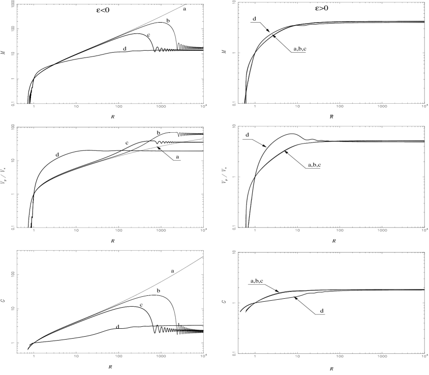
Figure 1: Plots of $M$ (upper panel), $V_{r}$ (in units of $V_{*}$, middle panel) and $G$ (lower panel) vs $R$ along the polar axis for $\epsilon/2\lambda^{2}=-0.1$ (left panel) and $0.25$ (right panel). Labels refer to different values of $\kappa=0$ (a), 0.001 (b), 0.003 (c) and 0.009 (d). In all these solutions we have selected the solution corresponding to $\Pi_{*}=\Pi_{*,\rm min}$.

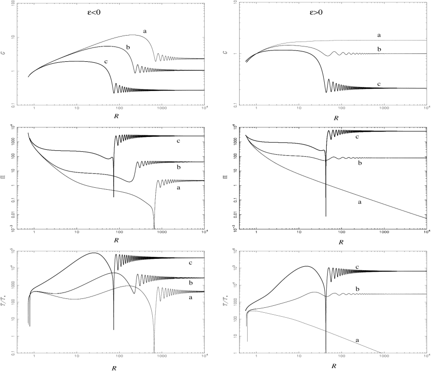
Figure 2: Plots of $G$ (upper panel), $\Pi$ (middle panel) and $T$ (lower panel) vs $R$ along the polar axis for $\kappa=0.003$ and $\epsilon/2\lambda^{2}=-0.1$ (left column) and $\epsilon/2\lambda^{2}=0.25$ (right column). Labels refer to different values of $\Pi_{*}$. For $\epsilon/2\lambda^{2}=-0.1$, $\Pi_{*}\approx 413$ (a, $\Pi_{*,\rm min}$), 420 (b), 653 (c, $\Pi_{*,max}$). For $\epsilon/2\lambda^{2}=0.25$, $\Pi_{*}\approx 297$ (a, $\Pi_{*,\rm min}$), 400 (b), 1135 (c, $\Pi_{*,max}$).

We remind that the parameters $\lambda$, $\delta$ and $\kappa$ are related to the strength of the rotational velocity, and to the structure of the density and of the pressure in the $\theta$ direction, respectively. For $\delta$ and $\kappa$ positive the density and pressure increase when receding from the polar axis. From the expression giving the base of the outflow $R_{o}$ as deduced from the definition of $\epsilon$ with $M_{0}=0$ and $G_{0}\ll 1$, Eq. (13):

$$R_{o}={{(\delta-\kappa)\nu^{2}/\lambda^{2}}\over{2-G^{2}_{o}-\epsilon/\lambda^{2}}}\,,$$ (14)

it is evident that the quantity $(\delta-\kappa)\nu^{2}$ rules the flow dynamics in the subAlfvénic region. Large values of it lead to steep initial acceleration, with the base of the flow close to the Alfvén surface. If $\delta=\kappa$, $R_{0}=0$ and there is no acceleration close to the base for a given speed at the Alfvén transition. We also see that we must have $\kappa<\delta$ in order that $R_{0}>0$ while $\delta>0$ ($\delta<0$) increases (decreases) the initial acceleration. For $\kappa>\delta$ the initial thermal driving of the outflow is not possible at the base (an analogous case was found in TTS97, where the quantity $\delta\nu^{2}$ had to be larger than a minimum threshold value to have mass ejection).

In the following two subsections we have fixed $\lambda=3$ and $\delta=0.01$ [with the value of $\nu$ deduced from Eq. 13] and analysed the trend of the solutions for different values of $\epsilon/2\lambda^{2}$, $\kappa/2\lambda^{2}$ and $\Pi_{*}$. A summary of all these properties is given in subsection (4.4) for $\lambda=\nu=1$.

4.2 Behaviour of the solutions with $\kappa$

In Figs. 1 we have plotted the Alfvén number $M(R)$, the radial velocity $V_{r}(R)$ along the polar axis and the jet radius $G(R)$ for $\epsilon/2\lambda^{2}=0.25$ and $-0.1$, and four different values of $\kappa=$ 0, 0.001, 0.003, 0.009. The chosen value of $\Pi_{*}$ is the minimum allowed ($\Pi_{*,\rm min}$), i.e. such that $\Pi$ is either vanishing asymptotically, or it is zero in the deepest minimum of the corresponding oscillations of the streamlines. With these assumptions we deduce the values of $\nu\approx 20\div 100$. The main parameters of the solutions are listed in Table 1.

In the subAlfvénic region ($R\mathbin{\raise 2.0pt\hbox{$<$}\hskip-9.0pt\lower 4.0pt\hbox{$\sim$}}1$), independently of the value of $\epsilon$, the increase of $\kappa$ rises the value of $F_{*}$ (i.e. the rate of expansion of the streamlines at $R=1$ is lower) and of the pressure: the outflow is ‘hotter’ and ‘narrower’ in the transAlfvénic region. For $\kappa=0\rightarrow 0.009$ $\Pi_{*,\rm min}\approx 200\div 2000$ (see Table 1). These effects however are evident only for $\epsilon<0$, while for positive $\epsilon$ the solutions are practically unaffected by the value of $\kappa$ (unless $\kappa\rightarrow\delta$, in which case oscillations of small amplitude occur and $R_{o}$ decreases). The location of the base of the flow $R_{o}$ is controlled by $(\delta-\kappa)\nu^{2}$. However in our plots the base of the flow does not change drastically except when $\kappa\rightarrow\delta$ (see Table 1). These trends are basically unaffected by the value of $\epsilon/2\lambda^{2}$.

In the superAlfvénic region ($R\mathbin{\raise 2.0pt\hbox{$>$}\hskip-9.0pt\lower 4.0pt\hbox{$\sim$}}1$), when $\epsilon>0$ the results are basically insensitive to an increase of the values of $\kappa$. The flow is always collimated as in ST94, while the radius of the jet is smoothly increasing. On the other hand, when $\epsilon<0$, the effect of $\kappa\neq 0$ is much more drastic. The outflow rapidly expands with $R$, reaches a maximum width and then it sharply recollimates to a rather narrow jet with large amplitude oscillations. For very small values of $\kappa$ ($\ll\delta$) this bump increases its amplitude while its position moves downwind. In the limiting case of $\kappa\rightarrow 0$, the bump is shifted to $R=\infty$ and the flow has radial streamlines. For $\kappa\rightarrow\delta$ the bump and the oscillations have shifted upstream and smoothed, and the solution becomes similar to the one with $\epsilon>0$. Note also that at the position of the bump the Alfvén number has a maximum (and the density is minimum), while the velocity is monotonically increasing and attains asymptotic values larger than in solutions with $\epsilon>0$.

Figure 3: Poloidal streamlines of some of the solutions discussed in Sec. 4 and in Fig. (1). The last solid line corresponds to the last streamline which is rooted to the star, while the dotted lines are connected to the surrounding disk.

4.3 Behaviour of the solutions with $\Pi_{*}$

The effect on the solutions of increasing the pressure at the Alfvén distance $\Pi_{*}$ to values $\Pi_{*}>\Pi_{*,\rm min}$ is shown in Fig. 2, where $G(R)$, $\Pi(R)$ and $T(R)$ are plotted for a positive and a negative value of $\epsilon$. First, we note that only for $\Pi_{*}\gg\Pi_{*,\rm min}$ the solutions with positive and negative $\epsilon$ appear to have similar profiles. And second, it is also evident that an increase of $\Pi_{*}$ always leads to a reduction of the jet radius, i.e. it has basically the same effect as the increase of $\kappa$ (Fig. 1). This is expected because the pressure gradient across the streamlines has terms which are $\propto\kappa\Pi$, Eq. (C). Nevertheless, the asymptotic Alfvén number and density are scarcely affected by the value of $\Pi_{*}$. And, the flow velocity ($\propto M^{2}/G^{2}$) increases with $\Pi_{*}$, a fact also related to an increase of the thermal driving efficiency.

Table 1: Parameters of the solutions for $\lambda=3$ and $\delta=0.01$. $R_{o}$ and $R_{cr}$ are given for $\Pi_{\star}=\Pi_{\star,\rm min}$.

$\epsilon/2\lambda^{2}=-0.1$
$\kappa$	$\Pi_{\star,\rm min}$	$\Pi_{\star,max}$	$R_{o}$	$R_{cr}$	$\nu$
0	289	-	0.72	0.72	34.1
0.001	321	505	0.73	0.73	35.9
0.003	413	653	0.73	0.74	40.3
0.009	1951	2089	0.79	0.97	102

$\epsilon/2\lambda^{2}=0.25$
$\kappa$	$\Pi_{\star,\rm min}$	$\Pi_{\star,max}$	$R_{o}$	$R_{cr}$	$\nu$
0	214	-	0.60	0.62	24.1
0.001	236	2007	0.61	0.62	25.2
0.003	297	1135	0.61	0.63	28.2
0.009	1286	1423	0.45	0.88	65.1

The pressure at the Alfvén surface $\Pi_{*}$ cannot be however arbitrarily large. Namely, the asymptotic pressure $\Pi_{\infty}$ increases with $\Pi_{*}$, and it may even exceed the corresponding pressure values at $R=1$, but there is a sharp decrease of $\Pi$ at the position of the bump (with a consequent lowering of the temperature). This minimum value of the pressure at the bump decreases by rising $\Pi_{*}$, and above a maximum value ($\Pi_{*,\rm max}$) the pressure becomes negative at the bump. Hence, acceptable solutions exist only for $\Pi_{*,\rm min}\leq\Pi_{*}\leq\Pi_{*,\rm max}$. In other words, the range of acceptable values of $\Pi_{*}$ is quite narrow, and further shrinks by decreasing $\epsilon/2\lambda^{2}$ and increasing $\kappa$ or $\delta$ (see Table 1). It turns out that below a threshold value of $\epsilon/2\lambda^{2}$ the solutions are unphysical because we obtain $\Pi_{*,\rm min}>\Pi_{*,\rm max}$, unless $\kappa\rightarrow\delta$. For example for $\epsilon/2\lambda^{2}=-5$ we have acceptable solutions only for $\kappa=0.009$ with $4750\leq\Pi_{*}\leq 4835$, besides the solution with $\kappa=0$ and radially expanding streamlines.

Concerning the asymptotic velocities of the collimated outflow, with the assumed parameters, as $\kappa=0.001\rightarrow 0.009$ and $\Pi_{*}=\Pi_{*,\rm min}\rightarrow\Pi_{*,\rm max}$ we find for $\epsilon/2\lambda^{2}=0.25$, $M=3.5\div 8$ and $V_{r}/V_{*}=5\div 5\times 10^{2}$, while for $\epsilon/2\lambda^{2}=-0.1$ we get $M=3\div 15$ and $V_{r}/V_{*}=20\div 4\times 10^{2}$ .

4.4 Summary of the parametric analysis

In order to summarize the trends we just discussed, we illustrate in Fig. 4 how the behaviour of the solutions with the pressure is displayed in the parameter space ($\epsilon$, $\kappa$) for an arbitrary and illustrative set of values $\lambda=\nu=1$. The exact location of the various domains in this space [$\epsilon$,$\kappa$] depends strongly on the set of the remaining parameters. The following discussion in each case refers to the solution corresponding to the minimum pressure $\Pi_{*,\rm min}$ allowed, except where it is otherwise indicated.

Figure 4: Summary of the various domains of the pressure behaviour in the parameter space [$\epsilon/2\lambda^{2}$, $\kappa/2\lambda^{2}$] for $\nu=\lambda=1$. We show the domains of magnetic collimation (stars), pressure confinement (crosses), the forbidden region where all collimated solutions obtain at the bumps a negative pressure (open squares), and finally the domain of the radial solutions (filled squares).

In the domain of Efficient Magnetic Rotators (EMR, $\epsilon>0$), jets are cylindrically collimated by magnetic forces, as expected (domain with stars in Fig. 4), unless $\kappa$ is getting too large in which case we enter the regime of pressure confinement (crosses in Fig. 4). This pressure confined region extends to the domain of Inefficient Magnetic Rotators (IMR) on the left part of Fig. 4. However, when $\epsilon$ is getting too negative, it occurs that $\Pi_{*,\rm min}>\Pi_{*,\rm max}$ for small enough values of $\kappa$ (open squares in Fig. 4). This region corresponds in principle to physically non acceptable collimated solutions; we shall see however in the following subsection that a subdomain exists where radial solutions may exist.

We remark that these main features of the numerical solutions we just discussed are not qualitatively affected by different values of the parameters. The main effect of lower values of $\lambda$ is to shift downstream the ‘X’ type critical point closer to the Alfvén point (see ST94), and the properties of the solutions appear very similar for equal values of the quantity $(\delta-\kappa)\nu^{2}$.

In the previous subsections, we have seen that slight increase of the magnitude of $\kappa$ and/or $\Pi_{*}$ sharply reduces the jet radius (mainly for $\epsilon<0$). The jet radius may even asymptotically become smaller than at $R=1$ (i.e., $G_{\infty}<1$). This configuration implies a reversal of the electric current somewhere in the superAlfvénic region, and this may still be consistent with a reasonable topological structure of the outflow (see e.g. VT98, Vlahakis 1998). However jets with such a decreased transverse size far from the central object are likely to be unrealistic. Therefore we could assume in general that the parameters should be constrained such that $G_{\infty}>1$. We must note also that when $G_{\infty}<1$ the asymptotic pressure is rather high (see Fig. 2) while it is reasonable to assume that in astrophysical jets $\Pi_{\infty}\ll\Pi_{*}$. From all these arguments it appears that collimated solutions suitable to model collimated astrophysical outflows should be in general selected with $\Pi_{*}\mathbin{\raise 2.0pt\hbox{$>$}\hskip-9.0pt\lower 4.0pt\hbox{$\sim$}}\Pi_{*,\rm min}$.

5 Limiting solutions

Figure 5: In the same parameter space as Fig. 4 we show the limiting solutions between the collimated solutions and the flaring ones which are either collimated without oscillations but negative $\Pi_{\infty}$ (circles) or which are radially expanding at least up to $R=10^{6}$ with $\Pi_{\infty}=0$ (filled squares)

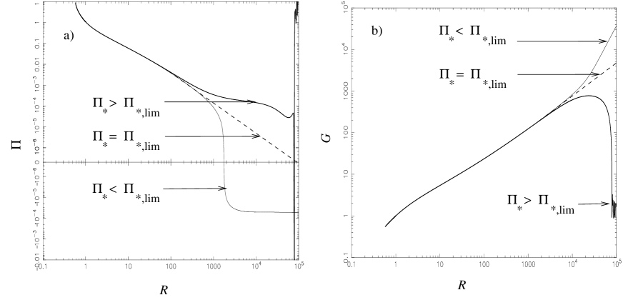
Figure 6: $\Pi(R)$ (panel a) and $G(R)$ (panel b) are plotted for $\epsilon/2\lambda^{2}=-0.5$, $\kappa=0.001$, $\nu=\lambda=1$. By tuning $\Pi_{*}$ to a special value $\Pi_{*}=\Pi_{*,\rm lim}$ we find, between a sharply recollimated ($\Pi_{*}>\Pi_{*,\rm lim}$) and a flaring solution ($\Pi_{*}<\Pi_{*,\rm lim}$), a limiting solution (dashed line) which is radial up to $R\approx 10^{6}$ (see the plot of the streamlines in Fig. 8a).

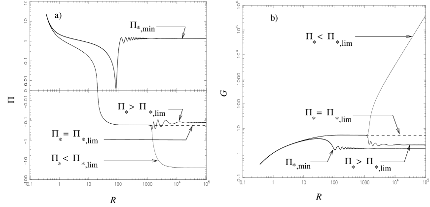
Figure 7: The same as in Fig. 6 for $\epsilon=0$, $\kappa=0.01$, $\nu=\lambda=1$: the limiting solution now is collimated without bumps. We plot also the solution with positive pressure everywhere, labeled with $\Pi_{*,\rm min}$. The streamlines of the limiting solution and of the one with $\Pi_{*}>\Pi_{*,\rm lim}$ are shown in Figs. 8b and 8c, respectively.

We outline here the properties of two kinds of solutions (that we call ‘limiting’ solutions) that are outside the boundary conditions on the pressure we discussed in the previous section.

5.1 Radially expanding limiting solutions

We have seen that for sufficiently negative values of $\epsilon$ and small values of $\kappa$, the sharp jet recollimation leads to a negative pressure, with $\Pi_{*,\rm min}$ becoming larger than $\Pi_{*,\rm max}$. These solutions have been rejected as unphysical (open squares in Fig. 4). However it turns out that by further decreasing $\Pi_{*}$ below $\Pi_{*,\rm min}$ we find a subdomain of this region (filled squares in Fig. 5), where we could follow numerically solutions that remain radial up to $R=10^{6}$ by tuning the initial pressure to a specific value $\Pi_{*}=\Pi_{*,\rm lim}$. An example of such a solution is given in Figs. 6 and 8a. These solutions, with an almost vanishing pressure and radial asymptotics, are limiting solutions between sharply recollimated ones (for $\Pi_{*}>\Pi_{*,\rm lim}$, see Fig. 6) and flaring solutions (for $\Pi_{*}<\Pi_{*,\rm lim}$). Numerically we are unable to say if such solutions are strictly radial asymptotically, or if they become cylindrical with a negative pressure far away from the base, as we discuss hereafter. However they can model radial winds up to the region of the outer asteropause where the wind is shocked with the interstellar medium because we do not expect the shock to be that far away (i.e. farther than $R=10^{6}$). Thus they allow some extension of the domain of radial winds into that of underpressured flows and they are well adapted to model winds like the solar wind (Lima et al. 2001a).

Figure 8: Sketch the poloidal streamlines of the radial limiting solution of Fig. 6 (panel a). In panels (b) and (c) we show the poloidal streamlines of the limiting solution (collimating without oscillations) and of the one sharply recollimated with $\Pi_{*}>\Pi_{*,\rm lim}$, reported in Fig. 7.

5.2 Non oscillating limiting solutions

In the remaining region of Fig. 5 (circles) the limiting solution between flaring and recollimating ones is a solution that collimates into cylinders without oscillations or bumps, and with negative $\Pi_{\infty}$. An example is presented in Figs. 7 and 8b. This result is not surprising and can be related to that obtained by TTS97, where two families of solutions were found for fixed streamlines. The first one was composed of thermally confined and underpressured jets showing the presence of a bump in the pressure. The second family was composed of initially underpressured jets which become overpressured downstream and magnetically confined without bumps. We have the analogous result here, at least in the domain of negative $\epsilon$.

But can this solution with negative $\Pi$ be acceptable? In fact, the pressure can be defined modulus an arbitrary constant,

$$P(R,\alpha)={1\over 2}\rho_{*}V^{2}_{*}\Pi(R)[1+\kappa\alpha]+P_{o}\,.$$ (15)

Thus we can drop the constraint $\Pi_{*}\geq\Pi_{*,\rm min}$ by choosing values of this constant such that the pressure is always positive. However the increase of $P$ implies also higher temperatures of the plasma, that should be eventually detectable with observations. Furthermore, high gas pressure could require unreasonable large heating processes in the plasma. So adding $P_{o}$ to solutions that present a bump in the pressure (as in Fig. 8c) is likely to be unrealistic. Conversely, including this constant to the limiting solutions with no bump (e.g. Fig. 8b) is feasible in principle and should not require a much larger amount of heating. We could speculate that such solutions could be interesting to model jets which are initially underpressured (in the region where $\Pi>0$) and overpressured in the outer zone (where $\Pi<0$).

6 Dynamics of the outflow

6.1 Force balance along and across the flow

A complete physical understanding of the behaviour of the solutions discussed in the previous section may be obtained by studying systematically the various forces acting on the outflow. In STT99 a similar analysis was attempted in asymptotically cylindrically collimated outflows. In such a case the jet had attained its terminal speed and force balance was studied only in the normal to the fieldlines direction. In the present case we consider all forces across and along the flow, in the whole region, from the base to the asymptotic zone. For this purpose, the original MHD set of equations can be projected on the poloidal plane and there they may be split in two directions, one being tangent ($\hat{s}$) and the other ($\hat{n}$) perpendicular to a particular poloidal streamline $\alpha=$ const. In this local system of orthogonal coordinates, the most general form of the MHD equations reduces to:

$$\parallel{\hat{s}}:\;\;0=-\rho V_{p}\frac{\partial V_{p}}{\partial s}-{\partial P\over\partial s}-\rho{\partial{\cal V}\over\partial s}+\left(\frac{\rho V^{2}_{\varphi}}{\varpi}-\frac{B^{2}_{\varphi}}{4\pi\varpi}\right){{\partial}\varpi\over{\partial}s}$$

$$-{{\partial}\over{\partial}s}\left(\frac{B^{2}_{\varphi}}{8\pi}\right)\,,\;\;\;\;\;\;$$ (16)

$$\parallel{\hat{n}}:\;\;0=-\frac{\rho V_{p}^{2}}{R_{c}}-{{\partial}P\over{\partial}n}-\rho{{\partial}{\cal V}\over{\partial}n}+\left(\frac{\rho V^{2}_{\varphi}}{\varpi}-\frac{B^{2}_{\varphi}}{4\pi\varpi}\right){{\partial}\varpi\over{\partial}n}$$

$$-{{\partial}\over{\partial}n}\left(\frac{B^{2}_{\varphi}}{8\pi}\right)-{{\partial}\over{\partial}n}\left(\frac{B^{2}_{p}}{8\pi}\right)+\frac{B^{2}_{p}}{4\pi R_{c}}\,,\;\;\;$$ (17)

where $\varpi=r\,{\rm sin}\theta$, ${\cal V}$ is the gravitational potential ($=-{\cal GM}/r$) and $R_{c}$ is the radius of curvature of the poloidal streamline. The vectors ${\hat{s}}$ and ${\hat{n}}$ are directed towards the outer regions and the polar axis, respectively. Then, a force $\@vec{f}$ has two components, $f^{\hat{s}}$ and $f^{\hat{n}}$. A positive component $f^{\hat{s}}$ accelerates the flow along the streamline, while a positive value for $f^{\hat{n}}$ collimates the plasma. Conversely, negative $f^{\hat{s}}$ and $f^{\hat{n}}$ imply that the wind is decelerated and that the streamlines ‘flare’ away from the axis, respectively.

The full expressions of the forces are given and discussed in detail in Appendix C. In the following we outline the main dynamical properties along and across the streamlines, referring to the cases of collimated flows we have discussed in Sec. 4 and plotted in Fig. 3.

6.2 Force balance along ${\hat{s}}$

It is easy to see that, the centrifugal force and the negative gas pressure gradient for a monotonically decreasing $\Pi(R)$, always accelerate the flow (see left panels of Figs. 9 - 12). On the other hand, gravity and the hoop stress associated with the toroidal magnetic field always decelerate the plasma. However the initially negative gradient of $B^{2}_{\varphi}/8\pi$ dominates close to the base and accelerates the flow (see left panels of Figs. 9 - 12). Finally, as is well known, the poloidal component of the magnetic field has no effect on the plasma dynamics along $\hat{s}$. From the left panels of Figs. 9 - 12, we see that the outflow is always thermally driven, with the magnetic and centrifugal forces playing a rather marginal role in the acceleration. For the assumed parameters the overall acceleration occurs for $R\mathbin{\raise 2.0pt\hbox{$<$}\hskip-9.0pt\lower 4.0pt\hbox{$\sim$}}10^{3}$, independently of the values of $\epsilon$ and $\kappa$. Oscillations in the flow variables may exist in some cases. For example, when $\epsilon<0$ and for intermediate values of $\kappa$ (Fig. 11), asymptotically the pressure gradient reacts to the oscillations of the streamlines, as expected in thermally confined jets (STT99). For larger values of $\kappa$ the flow appears already collimated in the acceleration region (see below), so the oscillations appear much closer to the Alfvénic surface (Figs. 10 and 12, left panels).

Figure 9: Plot of the different forces acting along ($\hat{s}$, left panel) and perpendicular to the poloidal streamlines ($\hat{n}$, right panel) for $\kappa=0.003$, $\epsilon/2\lambda^{2}=0.25$ and $\Pi_{*}=\Pi_{\rm min}$ (Fig. 3b). We plot the negative of the pressure gradient (dashes), the gravitational force (dash-three dots), the poloidal inertial and curvature forces (dots), the poloidal magnetic force (dash-dot), the centrifugal force (thin solid line) and the total toroidal magnetic force (thick solid line).

Figure 10: The same as Fig. 9 for $\kappa=0.009$, $\epsilon/2\lambda^{2}=0.25$ and $\Pi_{*}=\Pi_{\rm min}$ (Fig. 3d).

6.3 Force balance along ${\hat{n}}$

The analysis of the forces acting perpendicularly to a poloidal streamline is more complicated. First, the centrifugal force is always negative tending to open the streamlines. Second, both the tension and the gradient of the toroidal magnetic field are directed towards the axis, assisting collimation. Also, the normal component of the gravitational field tends to collimate the flow when the streamlines do not flare faster than the spherical expansion. Two terms contribute to the gradient of the pressure, with opposite effects: the term related to the radial component ($\propto{\rm d}\Pi/{\rm d}R$) decollimates the fieldlines while the one related to the meridional component ($\propto\kappa\Pi$) is positive and confines the flow. Concerning finally the poloidal magnetic field, its gradient is negative (decollimating) while its tension is positive (collimating).

The interplay of all these forces is shown in the right panels of Figs. 9 - 12. For positive $\epsilon$ and intermediate $\kappa$ (Fig. 9) the dynamics of the streamlines in the subAlfvénic and transAlfvénic region ($R\mathbin{\raise 2.0pt\hbox{$<$}\hskip-9.0pt\lower 4.0pt\hbox{$\sim$}}10$) is governed by gravity and the radial component of the pressure gradient. Farther away the magnetic and centrifugal forces prevail: the centrifugal force is balanced by the hoop stress and the gradient of the toroidal magnetic field (these two components provide the same contribution to this force). Asymptotically then the flow is magnetically confined (see also STT99). The effect of the other forces is quite negligible: they just show an oscillating behaviour that slightly affects the whole structure. This same picture basically holds if we increase the value of $\kappa$, with an increased effect of the thermal pressure (Fig. 10, right panel). Namely, the wind is always asymptotically magnetically collimated but in an intermediate region ($R\approx 15$) the outflow is thermally confined. Oscillations are always present in the subAlfvénic and the intermediate regions with larger amplitude: this is likely to be related to the larger effect of the pressure on a more collimated wind in this intermediate region.

A similar scenario is also found for negative $\epsilon$ and large values of $\kappa$ (see Fig. 12, right panel). The wind is also asymptotically magnetically collimated but with a larger intermediate region ($R\approx 20\div 100$) where the outflow is thermally confined.

For smaller $\kappa$ (Fig. 11, right panel), differently from the case with positive $\epsilon$, the toroidal magnetic force balances the curvature force in an intermediate region ($R\approx 10\div 100$) but without any confinement of the flow that expands almost radially in this zone. The collimation starts downwind where the gas pressure prevails on the magnetic force ($R\approx 100\div 400$), leading to a cylindrical configuration with oscillations (see Fig. 3a). In this asymptotic region the centrifugal force is balanced by the gradient of the pressure, with a small contribution from the toroidal magnetic field, since we are there in the thermally confined regime.

Figure 11: Plot of the different forces acting along ($\hat{s}$, left panel) and perpendicular to the poloidal streamlines ($\hat{n}$, right panel) for $\kappa=0.003$, $\epsilon/2\lambda^{2}=-0.1$ and $\Pi_{*}=\Pi_{\rm min}$ (Fig. 3a). As in Fig. 9 we plot the negative of the pressure gradient (dashes), the gravitational force (dash-three dots), the poloidal inertial and curvature forces (dots), the poloidal magnetic force (dash-dot), the centrifugal force (thin solid line) and the total toroidal magnetic force (thick solid line).

Figure 12: The same as Fig. 11 for $\kappa=0.009$, $\epsilon/2\lambda^{2}=-0.1$ and $\Pi_{*}=\Pi_{\rm min}$ (Fig. 3c).

7 Summary and astrophysical implications

In this paper we confined our attention to the study of outflows with a density increasing from the axis towards the surrounding streamlines [cf. Eq. (5) with $\delta>0$] faster than the pressure does [cf. Eq. (7) with $\kappa>0$], i.e. $\delta>\kappa$.

In such underpressured outflows, the temperature is peaked at the axis relatively to the surrounding regions. Such centrally hotter astrophysical atmospheres are likely to exist in coronae wherein, for example, strong Alfvén waves propagating along the direction of the polar magnetic field deposit enough energy which raises thus the plasma temperature. The inevitable consequence of this high temperature is an induced wind-type outflow, which is dominantly “thermally” driven around the rotation axis where magnetocentrifugal forces are negligible (see Figs. 9 - 12 ). By thermally we mean not only thermal conduction but also waves, etc, which can be effectively included in the pressure gradient term.

After the first acceleration stage where the gas expands almost radially up to the transAlfvénic region, if the outflow carries an electrical current and the magnetic rotator is sufficiently efficient (EMR), it is collimated magnetically via the combination of the hoop stress and the pressure gradient of the azimuthal magnetic field in the superAlfvénic regime. Several jets from Young Stellar Objects have probably such smoothly increasing radius with a large terminal transverse extension. They would naturally correspond to the magnetic collimation produced by an EMR. Outflows from an EMR may also describe jets from Radio Loud AGNs like FR Is and FR IIs (see Sauty et al. 2001 for a possible application of the present solutions to AGNs). For definite conclusions in this last case, however, a relativistic extension of our model is needed.

On the other hand, the produced outflow may also be collimated via thermal pressure gradients, if it is underpressured on the axis. Such pressure confined jets tend to show a rather strong recollimation. This could be related with some jets from slowly rotating T Tauri stars and Planetary Nebulae which show a rather strong recollimation, or some choked winds from Seyfert Galaxies. For example, the peculiar jet of RY Tauri originates in a very slowly rotating CTTS and seems to recollimate at 38 stellar radii from the base (see Gomez de Castro et al. 2001). The sharp gradient of the gas pressure in the recollimating region could lead naturally to the formation of a shock which may be consistent with the scenario of recollimation by internal shocks proposed in the literature.

In very Inefficient Magnetic Rotators (IMR) like the sun, radial solutions as the one plotted in Fig. 6 are likely to apply to winds produced by such sources (Lima et al. 2001b). Thus, jets from Young Stars may evolve from a narrowly collimated magnetic outflow to a radially expanding wind. Such radial solutions could also correspond to winds from Seyfert Galaxies.

If we were to apply recollimating solutions to jets from Planetary Nebulae, we would be inclined to think that in these objects recollimation is an effect of the pressure gradient rather than a pure magnetic pinching. Nevertheless, the jet could be ultimately magnetically confined once it has refocalized.

Interesting solutions for underpressured jets becoming overpressured after exiting from the central embedding medium can be found. They correspond to the limiting solution plotted in Figs. 7 and 8b. Such outflows are magnetically confined and in contrast with the previous ones do not exhibit any recollimation or oscillations. They may describe Young Stellar jets exiting from the central cloud.

More precise modelling of various specific astrophysical objects is underway and will be presented elsewhere; here we just summarize some of the results obtained so far. Preliminary applications to the solar wind are given in Lima et al. (2001b). By analysing Ulysses data we arrived at the following ranges of the model parameters for the solar wind : $\delta\approx 2-4$, $\lambda\approx 0.1$, $\kappa\approx 0.3-0.8$ and $\nu\approx 0.7$. With these parameters a reasonable fitting of all observed quantities is obtained, except perhaps the magnetic field at large distances, which turns out to be a bit too weak compared to the measured one. The above values of the parameters imply $\epsilon/2\lambda^{2}\sim-50$, thus confirming the strong inefficiency of the solar magnetic rotator. In such a case the solutions are expected to be qualitatively similar to those shown in Fig. 3a, i.e. radially expanding streamlines connected through the bump to the far dowstream collimated region. In the present case, with $\kappa\ll\delta$ and very low asymptotic pressure, the position of the bump is very far away from the Alfvénic surface, then the streamlines are expected to be basically radial in the region explored by the spacecraft.

Parallel to this, preliminary results for jets from T Tauri stars (Meliani 2001) provide the following range of the values of the parameters: $\delta\approx 0.1-0.2$, $\lambda\approx 0.8$, $\kappa\approx 0.01-0.06$, $\nu\approx 1-6$ and $r_{*}\approx 10\;r_{\star}\approx 20-30\;r_{\odot}$. It is worth noting that observations of these objects imply the existence of a UV emitting region near the central star, which may possibly be associated with a shock (e.g. in RY Tau this UV zone is at $\approx$ 38 $r_{\star}$). With the above parameters we deduce $\epsilon/2\lambda^{2}\approx 0$ (negative or positive), which means that T Tauri stars correspond to more efficient magnetic rotators. For the above ranges of the parameters, the solutions are expected to be similar to those reported in Fig. 7 and 8. In particular we could have a recollimated solution with the UV shock at the position of the bump, or a limiting solution with monotonically collimated streamlines without oscillations (see Fig. 8b), in which case the shock would result from the growth of some internal instability. Both types of solution reproduce in a satisfactory way the velocity and density profiles, the jet morphology and the rotational rate. Yet, the second type of solutions leads to lower temperature profiles which suggests that a thermally driven wind could account for the observed data in such objects, even without extra nonthermal heating.

To distinguish between recollimated and limiting solutions, we may ask about the stability of our solutions. Some hints about this crucial point can be given for the asymptotic region. By a local analysis using the thin flux tube approximation, Hanasz et al. (2000) have shown that the internal part of jets with rotational laws comparable to the one used in the present model (Eq.6) are more stable to magnetorotational instabilities than the surrounding jet coming from the disk. In some cases rotation completely suppress the instability. Of course, we do not claim that this analysis is complete but it may be an indication that azimuthal magnetic fields do not necessarily destroy the global structure of MHD outflows modelled by our solutions.

However, while the properties of the local stability of cylindrical jets are quite well known in the linear regime and for simple equilibrium structures (see e.g. Birkinshaw 1991, Ferrari 1998, and references therein, Kim & Ostriker 2000), unfortunately a global, non-linear analysis of the stability of general axisymmetric MHD steady flows is not yet available. This still remains a challenge for future studies. Furthermore, the present solutions may be used for the testing and interpretation of numerical codes employed for such a stability analysis.

To conclude with, let us stress that in the present study cylindrical jets and radial winds can carry a net current, at least in the central part close to the axis, because they are not necessarily force-free asymptotically. This is not in contradiction with the main conclusion in Heyvaerts & Norman (1989), because some of the approximations done there do not necessarily hold close to the axis. Our description is also only valid at the central part of the outflow, and the current should close either in the surrounding wind, the external medium, or in a current-carrying sheet around the jet.

Appendix A Generalities on self-similar solutions

For the sake of generality the free functions $A(\alpha)$, $\Psi_{A}(\alpha)$ and $\Omega(\alpha)$, can be defined through the following new functions (for details see VT98):

$$g_{1}(\alpha)\propto\int{\cal F}_{1}(A^{\prime}){\rm d}\alpha,\;\;\;\;\;g_{2}(\alpha)\propto\int\Omega^{2}\Psi^{2}_{A}{\rm d}\alpha,$$

$$g_{3}(\alpha)\propto{\cal F}_{2}(\Psi_{A})\,,$$ (18)

where $A^{\prime}\equiv{\rm d}A/{\rm d}\alpha$. We remark that $g_{1}$ is related to the magnetic field structure through the magnetic flux function, while $g_{2}$ and $g_{3}$ define the current and density distribution, respectively. Suitable choices of ${\cal F}_{1}$ and ${\cal F}_{2}$ allow to select various classes of self-similar solutions.

Radially self-similar models. If we assume $M\equiv M(\theta)$ (i.e. the surfaces with the same Alfvén number are conical), $G\equiv G(\theta)$ and in Eqs. (A.1):

$${\cal F}_{1}(A^{\prime})={{A^{\prime 2}}\over\alpha},\;\;\;\;{\cal F}_{2}(\Psi_{A})=\int{{\Psi^{2}_{A}}\over{\alpha^{3/2}}}{\rm d}\alpha\,,$$ (19)

we obtain a class of solutions that are self-similar in the radial direction, used to model outflows from disks. Assuming for instance $g_{1},g_{2},g_{3}\propto\alpha^{x}/(x-2)$ (see Table 3 in VT98) with $x=3/4$ we have the well known solutions of Blandford & Payne (1982).

Meridionally self-similar models. By choosing $G\equiv G(r)$, $M\equiv M(r)$ (i.e. the surfaces with the same Alfvén number are spherical) and:

$${\cal F}_{1}(A^{\prime})=A^{\prime 2},\;\;\;\;{\cal F}_{2}(\Psi_{A})=\Psi^{2}_{A}\,,$$ (20)

we obtain the class of $\theta-$ self-similar solutions. If we assume as the simplest case $g_{1}=\alpha$, $g_{2}=\lambda^{2}\alpha$ and $g_{3}=1+\delta\alpha$ ($\lambda$ and $\delta$ constants, see Table 1 in VT98 ) we get the solutions presented in ST94, TT97, STT99 and in the present paper.

Appendix B Equations for meridional self-similar flows)

From the definitions of Sec. 2.2 we deduce the following expressions for the three components of the velocity and magnetic field (for details see ST94):

$$B_{r}=B_{*}{1\over G^{2}(R)}\cos\theta\,,$$ (21)

$$B_{\theta}=-B_{*}{1\over G^{2}(R)}{F(R)\over 2}\sin\theta\,,$$ (22)

$$B_{\varphi}=-B_{*}{\lambda\over G^{2}(R)}{\displaystyle 1-G^{2}(R)\over 1-M^{2}(R)}{R\sin\theta}\,,$$ (23)

$$V_{r}=V_{*}{M^{2}(R)\over G^{2}(R)}{\cos\theta\over\sqrt{1+\delta\alpha(R,\theta)}},\;\;\;\;\;\;$$ (24)

$$V_{\theta}=-V_{*}{M^{2}(R)\over G^{2}(R)}{F(R)\over 2}{\sin\theta\over\sqrt{1+\delta\alpha(R,\theta)}}\,,$$ (25)

$$V_{\varphi}=V_{*}{\lambda\over G^{2}(R)}{G^{2}(R)-M^{2}(R)\over 1-M^{2}(R)}{R\sin\theta\over\sqrt{1+\delta\alpha(R,\theta)}}\,.$$ (26)

The three ordinary differential equations for $\Pi(R)$, $M^{2}(R)$ and $F(R)$ are:

$${\hbox{d}\Pi\over\hbox{d}R}=-{2\over G^{4}}\left[{\hbox{d}M^{2}\over\hbox{d}R}+{M^{2}\over R^{2}}(F-2)\right]-{\nu^{2}\over M^{2}R^{2}}\,,$$ (27)

$${\hbox{d}F(R)\over\hbox{d}R}={{{\cal N}_{F}(R,G,F,M^{2},\Pi;\kappa,\delta,\nu,\lambda)}\over\ {R\,{\cal D}(R,G,F,M^{2};\kappa,\lambda)}}\,,$$ (28)

$${\hbox{d}M^{2}(R)\over\hbox{d}R}={{{\cal N}_{M}(R,G,F,M^{2},\Pi;\kappa,\delta,\nu,\lambda)}\over\ {R\,{\cal D}(R,G,F,M^{2};\kappa,\lambda)}}\,,$$ (29)

where we have defined:

$${\cal D}=(M^{2}-1)\left(1+\kappa{R^{2}\over G^{2}}\right)+{F^{2}\over 4}+R^{2}\lambda^{2}{N_{B}^{2}\over D^{2}}\,,$$ (30)

$${\cal N}_{F}=-(\delta-\kappa)\nu^{2}{RG^{2}\over 2M^{2}}F$$

$$+\left({2\kappa\Pi G^{2}R^{2}}+(F+1)(F-2)\right)\times$$

$$\times\left(1+\kappa{R^{2}\over G^{2}}-{F^{2}\over 4}-R^{2}\lambda^{2}{N_{B}^{2}\over D^{3}}\right)$$

$$+{M^{2}F\over 4}(F-2)\left(F+2+2\kappa{R^{2}\over G^{2}}+2R^{2}\lambda^{2}{N_{B}^{2}\over D^{3}}\right)$$

$$-\lambda^{2}R^{2}F(F-2){N_{B}\over D^{2}}$$

$$+\lambda^{2}R^{2}\left(1+\kappa{R^{2}\over G^{2}}-R^{2}\lambda^{2}{N_{B}^{2}\over D^{3}}-{F\over 2}\right)$$

$$\left(4{N_{B}^{2}\over D^{2}}-{2\over M^{2}}{N_{V}^{2}\over D^{2}}\right)\,,$$ (31)

$${\cal N}_{M}=(\delta-\kappa)\nu^{2}{RG^{2}\over 2M^{2}}(M^{2}-1)$$

$$+\kappa\Pi R^{2}G^{2}M^{2}{F\over 2}-{M^{4}\over 4}(F-2)(4\kappa{R^{2}\over G^{2}}+F+4)$$

$$+{M^{2}\over 8}(F-2)(8\kappa{R^{2}\over G^{2}}+F^{2}+4F+8)$$

$$-\lambda^{2}R^{2}(F-2){N_{B}\over D}$$

$$+\lambda^{2}R^{2}(2M^{2}+F-2)\left({N_{B}^{2}\over D^{2}}-{1\over 2M^{2}}{N_{V}^{2}\over D^{2}}\right)\,.$$ (32)

with

$$N_{B}=1-G^{2},\;\;\;\;N_{V}=M^{2}-G^{2},\;\;\;\;D=1-M^{2}\,.$$ (33)

The meaning of the various parameters is discussed in Sec. 2.

At the Alfvén radius, the slope of $M^{2}(R=1)$ is $p=(2-F_{*})/\tau$, where $\tau$ is a solution of the third degree polynomial:

$$\tau^{3}+2\tau^{2}+\left[{{\kappa\Pi_{*}}\over{\lambda^{2}}}+{{F^{2}_{*}-4}\over{4\lambda^{2}}}-1\right]\tau+{{(F_{*}-2)F_{*}}\over{2\lambda^{2}}}=0\,,$$ (34)

and the star indicates values at $R=1$ (for details see ST94).

Appendix C Forces acting on the outflow on the poloidal plane

The components of the various MHD forces in the poloidal plane along the natural unit vectors ($\hat{n},\hat{s}$) are related to those along the spherical coordinates poloidal unit vectors ($\hat{r},\hat{\theta}$) via the following expressions:

$$f^{\hat{s}}(R,\theta)=f^{\hat{r}}\cos\chi(R,\theta)+f^{\hat{\theta}}\sin\chi(R,\theta)\,,$$ (35)

$$f^{\hat{n}}(R,\theta)=f^{\hat{r}}\sin\chi(R,\theta)-f^{\hat{\theta}}\cos\chi(R,\theta)\,,$$ (36)

Figure 13: Sketch of poloidal unit vectors for a converging ($\chi<0$) and a flaring ($\chi>0$) streamline (thick line).

with $\chi$ the angle a poloidal streamline makes with the radial direction $\hat{r}$ (Fig. 13). This angle is related to the expansion factor $F(R)$ and the polar angle $\theta$ as,

$$\tan\chi(R,\theta)=-\tan\theta\frac{F(R)}{2}\,.$$ (37)

When $\chi<0$ the poloidal streamline turns towards the symmetry axis, while when $\chi>0$ it flares faster than radiality (see Fig. 13). By taking into account Eqs. (B.1) - (B.6) for the dependence of the physical quantities on $r$ and $\theta$, we obtain the following expressions for the meridional components of the various MHD forces $f^{\hat{s}}$ and $f^{\hat{n}}$ plotted in Figs. 9 - 12. Note that all forces have the dimensions of $\rho_{*}V_{*}^{2}/2=B_{*}^{2}/4\pi$, a common factor which for simplicity we shall omit and the forces will thus be given dimensionless in the following (the different forces and their direction are listed in Table C1).

$\bullet$ Gravity: ${\@vec{f}}_{g}\equiv-\rho{\cal GM}/R^{2}\,\hat{r}$.

The two components of the gravitational force are:

$$f_{g}^{\hat{s}}\equiv-\rho{{\partial}{\cal V}\over{\partial}s}=-\cos\chi(R,\alpha){\nu^{2}\over M^{2}R^{2}}(1+\delta\alpha)\,,$$ (38)

$$f_{g}^{\hat{n}}\equiv-\rho{{\partial}{\cal V}\over{\partial}n}=-\sin\chi(R,\alpha){\nu^{2}\over M^{2}R^{2}}(1+\delta\alpha)\,.$$ (39)

Note that always $f^{\hat{s}}_{g}<0$, so that gravity in all cases acts to decelerate the flow, as expected. Conversely, $f^{\hat{n}}_{g}$ is positive and assists further a streamline which is turning toward the axis ($\chi<0$), while it is negative assisting further decollimation when $\chi>0$ and there is a flaring of the streamlines.

$\bullet$ Pressure gradient force: ${\@vec{f}}_{\@vec{\nabla}P}\equiv-\nabla P(R,\alpha)$.

The two components of the pressure gradient along and perpendicular to a poloidal streamline are:

$$f_{\nabla P}^{\hat{s}}\equiv-{{\partial}P\over{\partial}s}=-\cos\chi(R,\alpha){{\rm d}\Pi\over{\rm d}R}(1+\kappa\alpha)\,,$$ (40)

$$f_{\nabla P}^{\hat{n}}\equiv-{{\partial}P\over{\partial}n}=-\sin\chi(R,\alpha)\left\{\left[{\hbox{d}\Pi\over\hbox{d}R}+\frac{4\kappa R\Pi}{FG^{2}}\right]\right.$$

$$+\kappa\alpha\left.\left[{{\rm d}\Pi\over{\rm d}R}+\frac{4\Pi}{FR}\left(\frac{F^{2}}{4}-1\right)\right]\right\}\,.$$ (41)

Note that $f_{\nabla P}^{\hat{s}}$ is always positive driving thus the wind whenever $\Pi$ decreases monotonically with $R$, as for example close to the hot base of the outflow (Figs. 9 - 12, left panels). In the strongly oscillating regions $f_{\nabla P}^{\hat{s}}$ periodically accelerates and decelerates the wind. The behaviour of the perpendicular component $f_{\nabla P}^{\hat{n}}$ is more complex because it depends also on the strength of $\kappa\Pi$. In the transAlfvénic region the pressure gradient is large, so that:

$$f_{\nabla P}^{\hat{n}}\approx-\sin\chi(R,\alpha)(1+\kappa\alpha){{\rm d}\Pi\over{\rm d}R}\,,$$ (42)

while for $R\gg 1$, ${\rm d}\Pi/{\rm d}R\rightarrow 0$ and

$$f_{\nabla P}^{\hat{n}}\approx-\frac{4\kappa R}{FG^{2}}\Pi\sin\chi(R,\alpha)\,.$$ (43)

Hence, it becomes evident why in the subAlfvénic ($R<1$) and transAlfvénic ($R\mathbin{\raise 2.0pt\hbox{$>$}\hskip-9.0pt\lower 4.0pt\hbox{$\sim$}}1$) regions the gradient of the gas pressure acts to ‘open’ the fieldlines ($f_{\nabla P}^{\hat{n}}<0$), while further away ($R\gg 1$) the term $\propto\kappa\Pi$ acts to assist collimation for $\kappa>0$ ($f_{\nabla P}^{\hat{n}}>0$).

Table 2: Forces acting on a converging ($\chi<0$) and a flaring ($\chi>0$) streamline: they are parallel or antiparallel to the unit vectors $\hat{s}$ and $\hat{n}$ when they are $>0$ or $<0$, respectively. Then positive or negative $f^{\hat{s}}$ means that it accelerates or decelerates the flow, while positive or negative $f^{\hat{n}}$ means that it collimates or decollimates. Conversely $f_{V_{p}}^{\hat{s}}<0$ corresponds to acceleration and $f_{V_{p}}^{\hat{s}}>0$ to deceleration.

Force	Components	Conv. str. ($\chi<0$)	Flar. str. ($\chi>0$)
Gravity	$f_{g}^{\hat{s}}\equiv-\rho{{{\partial}{\cal V}}\over{{\partial}s}}$	$<0$	$<0$
	$f_{g}^{\hat{n}}\equiv-\rho{{{\partial}{\cal V}}\over{{\partial}n}}$	$>0$	$<0$
Pressure Gradient	$f_{\nabla P}^{\hat{s}}\equiv-{{{\partial}P}\over{{\partial}s}}$	$>0$	$>0$
	$f_{\nabla P}^{\hat{n}}\equiv-{{{\partial}P}\over{{\partial}n}}$	$<0$ $(|{\rm d}\Pi/{\rm d}R|\gg 0)$	$>0$ $(|{\rm d}\Pi/{\rm d}R|\gg 0)$
		$>0$ $({\rm d}\Pi/{\rm d}R\rightarrow 0)$	$<0$ $({\rm d}\Pi/{\rm d}R\rightarrow 0)$
Centrifugal Force	$f_{V_{\varphi}}^{\hat{s}}\equiv{{\rho V^{2}_{\varphi}}\over{\varpi}}{{{\partial}\varpi}\over{{\partial}s}}$	$>0$	$>0$
	$f_{V_{\varphi}}^{\hat{n}}\equiv{{\rho V^{2}_{\varphi}}\over\varpi}{{{\partial}\varpi}\over{{\partial}n}}$	$<0$	$<0$
Magn. hoop stress of $B_{\varphi}$	$T_{B_{\varphi}}^{\hat{s}}\equiv-{{B^{2}_{\varphi}}\over{4\pi\varpi}}{{{\partial}\varpi}\over{{\partial}s}}$	$<0$	$<0$
	$T_{B_{\varphi}}^{\hat{n}}\equiv-{{B^{2}_{\varphi}}\over{4\pi\varpi}}{{{\partial}\varpi}\over{{\partial}n}}$	$>0$	$>0$
Magn. pressure grad. of $B_{\varphi}$	$f_{\nabla B_{\varphi}}^{\hat{s}}\equiv-{{\partial}\over{{\partial}s}}\left({{B^{2}_{\varphi}}\over{8\pi}}\right)$	$>0$ or $<0$	$>0$ or $<0$
	$f_{\nabla B_{\varphi}}^{\hat{n}}\equiv-{{\partial}\over{{\partial}n}}\left({{B^{2}_{\varphi}}\over{8\pi}}\right)$	$>0^{\rm a}$	$>0^{\rm a}$
Poloidal inertial force	$f_{V_{p}}^{\hat{s}}\equiv-\rho V_{p}{\partial V_{p}\over\partial s}$	$<0$	$<0$
	$f_{V_{p}}^{\hat{n}}\equiv-\frac{\rho V_{p}^{2}}{R_{c}}$	$<0$	$>0$
Magn. hoop stress of $B_{p}$	——	——	——
	$T_{B_{p}}^{\hat{n}}\equiv{{B_{p}^{2}}\over{4\pi R_{c}}}$	$>0$	$<0$
Magn. pressure grad. of $B_{p}$	——	——	——
	$f_{\nabla B_{p}}^{\hat{n}}\equiv-{{\partial}\over{{\partial}n}}\left({{B_{p}^{2}}\over{8\pi}}\right)$	$<0$	$>0$

^a Only for $B_{\varphi}$ monotonically increasing with $\varpi$

$\bullet$ Centrifugal ‘force’: ${\@vec{f}}_{V_{\varphi}}={\hat{\varpi}}(\rho V^{2}_{\varphi}/\varpi)$.

This centrifugal ‘force’ is always directed outwards, in the $+{\hat{\varpi}}$ direction with components :

$$f_{V_{\varphi}}^{\hat{s}}\equiv{{\rho V^{2}_{\varphi}}\over{\varpi}}{{{\partial}\varpi}\over{{\partial}s}}=\cos\chi(R,\alpha){2\lambda^{2}\over RG^{2}M^{2}}\left[{M^{2}-G^{2}\over 1-M^{2}}\right]^{2}$$

$$\times\left(1-\frac{F}{2}\right)\alpha\,,\;\;\;\;\;$$ (44)

$$f_{V_{\varphi}}^{\hat{n}}\equiv{{\rho V^{2}_{\varphi}}\over\varpi}{{{\partial}\varpi}\over{{\partial}n}}=\sin\chi(R,\alpha){4\lambda^{2}\over FRG^{2}M^{2}}\left[{M^{2}-G^{2}\over 1-M^{2}}\right]^{2}$$

$$\times\left[\frac{R^{2}}{G^{2}}+\alpha\left(\frac{F}{2}-1\right)\right]\,.\;\;\;\;\;$$ (45)

We see that always $f_{V_{\varphi}}^{\hat{s}}>0$, such that the centrifugal ‘force’ acts towards accelerating the flow, as a ‘bead sliding along a rotating wire’ in the picture of Blandford & Payne (1982). On the other hand, we have $f_{V_{\varphi}}^{\hat{n}}<0$ such that the centrifugal ‘force’ tends to further decollimate the streamlines, for all angles $\theta$ when the poloidal streamlines are deflected from radiality towards the polar axis ($\chi<0$, or, $0<F<2$) and also for small polar angles $\theta$ satisfying $\tan^{2}\theta<2/(-F)$, or, $\tan^{2}\chi<(-F)/2$ when the streamlines flare towards the equator ($\chi>0$, or, $F<0$).

$\bullet$ Toroidal magnetic force, $\@vec{f}_{B_{\varphi}}\equiv(\@vec{\nabla}\times\@vec{B}_{\varphi})\times\@vec{B}_{\varphi}$.

The toroidal magnetic force $\@vec{f}_{B_{\varphi}}$ has two components, a tension $\@vec{T}_{B_{\varphi}}$ and a toroidal magnetic pressure gradient, $\@vec{f}_{\nabla B_{\varphi}}$, both appearing in Eqs. (6.1) and (6.1).

$\bullet$ Magnetic hoop stress of $B_{\varphi}$ : ${\@vec{T}}_{B_{\varphi}}={\hat{\varpi}}(B^{2}_{\varphi}/4\pi\varpi)$.

The tension of the toroidal magnetic field is in a direction opposite to the centrifugal ‘force’, i.e., it acts in the $-{\hat{\varpi}}$ direction with components :

$$T_{B_{\varphi}}^{\hat{s}}\equiv-{{B^{2}_{\varphi}}\over{4\pi\varpi}}{{{\partial}\varpi}\over{{\partial}s}}=-\cos\chi(R,\alpha){2\lambda^{2}\over RG^{2}}\left[{1-G^{2}\over 1-M^{2}}\right]^{2}$$

$$\times\left(1-\frac{F}{2}\right)\alpha\,,\;\;\;\;\;$$ (46)

$$T_{B_{\varphi}}^{\hat{n}}\equiv-{{B^{2}_{\varphi}}\over{4\pi\varpi}}{{{\partial}\varpi}\over{{\partial}n}}=-\sin\chi(R,\alpha){4\lambda^{2}\over FRG^{2}}\left[{1-G^{2}\over 1-M^{2}}\right]^{2}$$

$$\times\left[\frac{R^{2}}{G^{2}}+\alpha\left(\frac{F}{2}-1\right)\right]\,.\;\;\;\;\;\;\;\;$$ (47)

Thus, we see that always $T_{B_{\varphi}}^{\hat{s}}<0$, such that the hoop stress acts towards decelerating the flow. On the other hand, we have $T_{B_{\varphi}}^{\hat{n}}>0$ such that the toroidal magnetic stress tends to collimate the streamlines when the poloidal streamlines are deflected from radiality towards the polar axis ($\chi<0$, or, $0<F<2$) and also for small polar angles $\theta$ satisfying $\tan^{2}\theta<2/(-F)$, or, $\tan^{2}\chi<(-F)/2$ when they flare towards the equator ($\chi>0$, or, $F<0$).

$\bullet$ Magnetic pressure gradient of $B_{\varphi}$: ${\@vec{f}}_{\nabla B_{\varphi}}=-\nabla(B^{2}_{\varphi}/8\pi)$.

This force is positive or negative depending on whether $B_{\varphi}$ decreases or increases with ${\hat{\varpi}}$, respectively. Its components are:

$$f_{\nabla B_{\varphi}}^{\hat{s}}\equiv-{{\partial}\over{{\partial}s}}\left({{B^{2}_{\varphi}}\over{8\pi}}\right)=-\cos\chi(R,\alpha){2\lambda^{2}\over RG^{2}}{1-G^{2}\over(1-M^{2})^{2}}$$

$$\times\left[\left(\frac{F}{2}-1\right)\left(G^{2}+1\right)+R{1-G^{2}\over 1-M^{2}}{{d}M^{2}\over{d}R}\right]\alpha\,,\;\;\;\;$$ (48)

$$f_{\nabla B_{\varphi}}^{\hat{n}}\equiv-{{\partial}\over{{\partial}n}}\left({{B^{2}_{\varphi}}\over{8\pi}}\right)=-\sin\chi(R,\alpha){4\lambda^{2}\over FRG^{2}}{1-G^{2}\over(1-M^{2})^{2}}$$

$$\times\left\{\frac{R^{2}}{G^{2}}(1-G^{2})+\left[\frac{FR}{2}{1-G^{2}\over 1-M^{2}}{{d}M^{2}\over{d}R}\right.\right.$$

$$\left.\left.+\left(\frac{F}{2}-1\right)\left(F-G^{2}+1\right)\right]\alpha\right\}\,.\;\;\;\;\;\;\;\;$$ (49)

In the accelerating initial region $B_{\varphi}$ decreases with $R$ and thus with $\varpi$ so the positive gradient of the toroidal magnetic field accelerates the flow. In the case of collimated flows $B_{\varphi}$ increases with $\varpi$ so the negative gradient of the toroidal magnetic field acts in the same direction as the hoop stress, collimating and decelerating the wind. Note that it is easy to see that the meridional components of the tension and the gradient of $B_{\varphi}$ have an equal amplitude.

$\bullet$ The poloidal flow inertial and curvature forces, $\@vec{f}_{V_{p}}\equiv-\rho({\@vec{V}_{p}}\cdot\nabla){\@vec{V}_{p}}$.

The two components of this force are:

$$f_{V_{p}}^{\hat{s}}\equiv-\rho V_{p}{\partial V_{p}\over\partial s}=-{2\cos\chi(R,\alpha)\over G^{4}}\left\{\left[{{d}M^{2}\over{d}R}+\frac{M^{2}}{R}(F-2)\right]\right.$$

$$+\alpha\left[\frac{G^{2}}{R^{2}}\left(\frac{F^{2}}{4}-1\right){dM^{2}\over dR}\right.$$

$$\left.\left.+{M^{2}G^{2}\over 4R^{3}}\left({F^{3}\over 2}-2F^{2}-2F+8+RF{{d}F\over{d}R}\right)\right]\right\}\,.\;\;\;\;\;\;\;\;$$ (50)

$$f_{V_{p}}^{\hat{n}}\equiv-\frac{\rho V_{p}^{2}}{R_{c}}=\sin\chi(R,\alpha)\frac{2M^{2}}{FRG^{4}}\left[\left(R{dF\over dR}-\frac{F^{2}}{2}+F\right)\right.$$

$$\left.+{\alpha G^{2}\over R^{2}}\left({F^{3}\over 4}-F-R{{d}F\over{d}R}\right)\right]\,,\;\;\;\;\;\;\;\;$$ (51)

where $R_{c}$ is the local radius of curvature. Along a poloidal streamline, $f_{V_{p}}^{\hat{s}}$ balances all other forces along $\hat{s}$ on the poloidal plane. Obviously, when the poloidal flow inertial force $-f_{V_{p}}^{\hat{s}}$ is positive the flow is accelerated, as in the inner region, while when it is negative the flow decelerates, as when oscillations are present. Perpendicularly to a poloidal streamline, i.e. along $\hat{n}$, the poloidal flow curvature force $-f_{V_{p}}^{\hat{n}}$ is positive when the streamlines turn towards the axis (as in the inner region), zero in the radial case and negative when there is some flaring away from radiality (e.g., in the oscillating zone).

$\bullet$ Poloidal magnetic force, $\@vec{f}_{B_{p}}\equiv(\@vec{\nabla}\times\@vec{B}_{p})\times\@vec{B}_{p}$.

This force is directed only normal to the poloidal magnetic fieldlines, since its $\hat{s}-$component does not appear in Eq. (6.1). As for $B_{\varphi}$, the poloidal magnetic force has two components, a tension $T^{\hat{n}}_{B_{p}}$ and a poloidal magnetic pressure gradient, $f^{\hat{n}}_{\nabla B_{p}}$, both appearing in Eq. (6.1).

$\bullet$ Magnetic hoop stress of $B_{p}$: $T^{\hat{n}}_{B_{p}}$ $\equiv\hat{n}\cdot({\@vec{B}_{p}}\cdot\nabla){\@vec{B}_{p}}/4\pi$.

This force is focusing the streamlines towards the axis when they collimate and towards the equatorial plane when they are flaring:

$$T_{B_{p}}^{\hat{n}}\equiv\frac{B_{p}^{2}}{4\pi R_{c}}=-\sin\chi(R,\alpha)\frac{2}{FRG^{4}}\left[\left(R{\hbox{d}F\over\hbox{d}R}-\frac{F^{2}}{2}+F\right)\right.$$

$$\left.+{\alpha G^{2}\over R^{2}}\left({F^{3}\over 4}-F-R{{d}F\over{d}R}\right)\right]\,.\;\;\;\;\;\;\;$$ (52)

Note that in the regime of the oscillations this poloidal magnetic curvature force is in opposite phase with the poloidal velocity curvature force. However, the ratio of their amplitude equals to $M^{2}$ and thus in highly superAlfvénic outflows ($M\gg 1$), the poloidal magnetic curvature force is negligible in comparison to the poloidal flow curvature force.

$\bullet$ Magnetic pressure grad. of $B_{p}$: $f_{\nabla B_{p}}^{\hat{n}}$ $\equiv-\hat{n}\cdot\@vec{\nabla}\left({B_{p}}^{2}/8\pi\right)$.

The pressure gradient of the poloidal magnetic field reads as:

$$f_{\nabla B_{p}}^{\hat{n}}\equiv-{{\partial}\over{\partial}n}\left(\frac{B^{2}_{p}}{8\pi}\right)=\sin\chi(R,\alpha)\left\{{2(2-F)\over RG^{4}}\right.$$

$$\left.-\frac{4}{FG^{2}R^{3}}\left(\frac{F^{2}}{4}-1\right)-{\alpha\over G^{2}R^{2}}\left[\frac{F}{2}{{d}F\over{d}R}\right.\right.$$

$$\left.\left.+\frac{2(F-2)}{R}\left(\frac{F^{2}}{4}-1\right)\right]+\frac{4\alpha}{FR^{5}}\left(\frac{F^{2}}{4}-1\right)\right\}\,.\;\;\;\;$$ (53)

In an almost radial expansion $B_{p}$ drops rather fast with $R$, $B_{p}\sim R^{-2}$ and thus $f_{\nabla B_{p}}^{\hat{n}}$ has a strong component along the radial direction. In such cases, the gradient of the poloidal magnetic pressure has a component along -$\hat{n}$ acting to decollimate the outflow. In fact, this strong poloidal magnetic pressure gradient when combined with the rather weak poloidal magnetic curvature force for superAlfvénic flows, results in a total poloidal magnetic force which has roughly the magnitude and sign of $\@vec{f}_{\nabla B_{p}}^{\hat{n}}$, Figs. 9-12.