Inflation and non–Gaussianity

Abstract

We study non-Gaussian signatures on the cosmic microwave background (CMB) radiation predicted within inflationary models with non-vacuum initial states for cosmological perturbations. The model incorporates a privileged scale, which implies the existence of a feature in the primordial power spectrum. This broken-scale-invariant model predicts a vanishing three-point correlation function for the CMB temperature anisotropies (or any other odd-numbered-point correlation function) whilst an intrinsic non-Gaussian signature arises for any even-numbered-point correlation function. We thus focus on the first non-vanishing moment, the CMB four-point function at zero lag, namely the kurtosis, and compute its expected value for different locations of the primordial feature in the spectrum, as suggested in the literature to conform to observations of large scale structure. The excess kurtosis is found to be negative and the signal to noise ratio for the dimensionless excess kurtosis parameter is equal to $|S/N|\simeq 4\times 10^{-4}$, almost independently of the free parameters of the model. This signature turns out to be undetectable. We conclude that, subject to current tests, Gaussianity is a generic property of single field inflationary models. The only uncertainty concerning this prediction is that the effect of back-reaction has not yet been properly incorporated. The implications for the trans-Planckian problem of inflation are also briefly discussed.

I Introduction

The theory of inflation is presently the most appealing candidate for describing the early universe. Inflation essentially consists of a phase of accelerated expansion which took place at a very high energy scale. One of the main reasons for such an appeal is the fact that inflation is deeply rooted in the basic principles of general relativity and field theory, which are well-tested theories. It is because all the forms of energy gravitate in general relativity that one of them, the pressure, which can be negative in field theory, is able to cause the acceleration in the expansion of the universe. In addition, when the principles of quantum mechanics are taken into account, inflation provides a natural explanation for the origin of the large scale structures and the associated temperature anisotropies in the Cosmic Microwave Background (CMB) radiation ruthhuscott .

Inflation makes four key predictions: (i) the curvature of the space-like sections vanishes, i.e. the total energy density, relative to the critical density, is $\Omega_{0}=1$, (ii) the power spectrum of density fluctuations is almost scale invariant, i.e. its spectral index is $n_{{}_{\rm S}}\simeq 1$, (iii) there is a background of primordial gravitational waves (which is also scale invariant), and (iv) the statistical properties of the CMB are Gaussian. In this article we focus on the last prediction and investigate whether it is a robust and generic property of inflationary models. The statistical properties of the CMB will be measured with high accuracy by the MAP and Planck satellites sate . So far the preliminary measurements of the three- and four-point correlation functions nongau3 ; nongau4 ; nongauss5 seem to be consistent with Gaussianity.

The fact that the statistical properties of the CMB are Gaussian can be directly traced back to the common assumption that the quantum fluctuations of the inflaton field are placed in the vacuum state Grishchuk-Martin . Therefore, in order to answer the above question, one has to investigate which kind of non-Gaussianity shows up if the vacuum state assumption is relaxed lps ; MRS ; devega ; con . In particular, one crucial point is to study whether this modification yields a detectable signal for future CMB or large-scale structure observations. Let us also notice that there exist other mechanisms to produce non-Gaussianity within the framework of inflation. Some of them have been studied in Refs. linde ; mat .

Assuming that the quantum state of the perturbations is a non-vacuum state immediately leads to the following difficulty: non-vacuum initial states imply, in general, a large energy density of inflaton field quanta, not of a cosmological term type ll . In other words, generically, if the initial state is not the vacuum then there is a back-reaction problem that could upset the inflationary phase. However, as we will argue below, one cannot directly conclude that this would prevent inflation from occurring altogether because, without a detailed calculation, it is difficult to guess what the back-reaction effect on the background would be. Such a detailed calculation is in principle possible by means of the formalism developed in Ref. Abramo . To our knowledge, such a computation has never been performed. The calculation of second order effects is clearly a complicated issue and is still the subject of discussions in the literature, see Unruh for example. Moreover there exist situations where it can be avoided, and this is in fact the case if the number of e-folds is not too large. In this article, we will not address the general question mentioned above but will rather concentrate on the more modest aim of calculating the non-Gaussianity in a case where the back-reaction problem is not too severe, hoping in this way to capture some features of the real situation.

There exist other arguments to study the non-Gaussianity that arises from a non-vacuum state. One of these is the so-called trans-Planckian problem of inflation jeroandCo : the quantum fluctuations are typically generated from sub-Planckian scales and therefore the predictions of inflation depend in fact on hidden assumptions about the physics on length scales smaller than the Planck scale. However, it has recently been shown that inflation is robust to some changes of the standard laws of physics beyond the Planck scale. More precisely, inflation is robust to a modification of the dispersion relation, at least if those changes are not too drastic, in practice if the Wigner-Kramer-Brillouin (WKB) evolution of the cosmological perturbations is preserved. However, modeling trans-Planckian physics by a change in the dispersion relation is clearly ad-hoc. Therefore, it is interesting to consider other possibilities; for example, one could imagine that the inflaton field emerges from the trans-Planckian regime in a non-vacuum state. Non-Gaussianity would then be, in this case, a signature of non standard physics and it seems to us interesting to quantify this effect. Let us note that similar ideas have been suggested in Ref. Chu in a slightly different context. Let us also remark that it has been shown recently in Ref. HKi that placing the cosmological perturbations in a non-vacuum state would lead to possible observable effects, for instance a modification of the consistency check of inflation.

Another motivation for calculating non-Gaussianity when the initial state is not the vacuum is that this model could be used to test the methods that are being developed to detect non-Gaussianity in the future CMB maps. There have been approaches based on the $n$th order moments or the cumulants of the temperature distribution pedro , the n-point correlation functions or their spherical harmonic transforms sht , and also works based on the detection of gradients in the wavelet space ag1 , to mention just a few methods. In the last approach, namely the wavelet analysis of a signal ag1 , the test maps which were employed were characterized by a non-skewed non-Gaussian distribution. Therefore, any non-Gaussianity was indicated by a non-zero excess kurtosis of the coefficients associated with the gradients of the signal. As we will show, this is exactly our case. This wavelet analysis of a signal was then applied ag2 to search for the CMB non-Gaussian signatures. More precisely, these authors investigated the detectability of a non-Gaussian signal induced by secondary anisotropies, while assuming Gaussian-distributed primary anisotropies. Their method ag2 is unable to detect such non-Gaussianity for the MAP-like instrumental configuration while it can do it for Planck-like capabilities.

From the theoretical point of view the simplest way to generalize the vacuum initial state, which contains no privileged scale, is to consider an initial state with a built-in characteristic scale, $k_{\rm b}$  MRS . Here, we will consider a non-vacuum state which is simpler and more generic than the one considered in this previous work. Several observables can be used to constrain the parameter space. A first possibility is to use the CMB anisotropy multipole moments to constrain the number of quanta $n$ around the privileged scale. It has been shown in Ref. MRS that, typically, this number cannot be large and in the present article we will always consider that $n$ is a few. With the recent release of the BOOMERanG boom , MAXIMA max and DASI dasi data, which revealed the existence of a first acoustic peak in the angular power spectrum at $\ell\sim 200$, followed by a second acoustic peak located at $\ell\sim 500$ and an evidence for a third peak, one can hope to obtain stronger constraints on $k_{\rm b}$ and $n$ very soon. Of course, another observable which can also be used is the matter density power spectrum. We will compare the predictions of our model for different cosmologies with the result of recent observations below.

The model we are studying here belongs to a class with a Broken Scale Invariant (BSI) power spectrum for the matter density. Such a primordial spectrum could also be generated ace during an inflationary era where the inflaton potential is endowed with steps, e.g., induced by a spontaneous symmetry breaking phase transition. The main motivation behind this class of models comes from Abell/ACO galaxy cluster redshift surveys which indicate einasto that the matter power spectrum seems to contain large amplitude features close to a scale of $100h^{-1}\rm Mpc$ (see however  diegoGL ). In support of this finding are the preliminary results of the recently released qso ; gary power spectrum analysis of the redshift surveys of Quasi-Stellar Objects (QSOs). Using the 10k catalogue from the 2dF QSO Redshift Survey croom , it has been tentatively identified qso a “spike” feature at a scale $\approx 90h^{-1}$Mpc ($\approx 65h^{-1}$Mpc) assuming a Lambda contribution $\Omega_{\rm\Lambda}=0.7$ and an ordinary matter contribution $\Omega_{\rm m}=0.3$ (respectively, $\Omega_{\rm\Lambda}=0$ and $\Omega_{\rm m}=1.0$). Provided this feature is confirmed, it might also have originated from acoustic oscillations in the tightly-coupled baryon-radiation fluid prior to decoupling. Using the CMBFAST code it was found qso that this spike in the spectrum is seen at a $\geq 25$ per cent smaller wavenumber than the second acoustic peak, while higher values of the baryon contribution $\Omega_{\rm b}$ may be needed to fit the amplitude of this feature. If we interpret this feature as originating from the primordial spectrum then, in order to be consistent with observations, the preferred scale $k_{\rm b}$ must lie way below the horizon today, possibly at a scale corresponding to the turn of the power spectrum einasto or at the scale matching the first acoustic peak of the CMB temperature anisotropies  silk . One then sees that the presently available data already restricts the parameter space for the quantities $k_{\rm b}$ and $n$ susana .

For the class of models which contain a preferred scale, a generic prediction is that the three-point correlation function vanishes (as well as any higher-order odd-point function), whereas the four-point (as well as any higher-order even-point) correlation function no longer satisfies the relation

$$\biggl{\langle}\biggl{(}\frac{\delta T}{T}\biggr{)}^{4}\biggr{\rangle}=3\biggl{\langle}\biggl{(}\frac{\delta T}{T}\biggr{)}^{2}\biggr{\rangle}^{2}~{},$$ (1)

which is typical of Gaussian statistics. Since the third-order moment (the skewness) vanishes, a first step is to calculate the fourth-order statistics (the kurtosis). It is interesting to perform this calculation for very large (COBE-size) angular scales, for which one can be confident that the source of non-Gaussianity is primordial. On the other hand, if the non-Gaussian signature was calculated on intermediate scales, a stronger signal would be obtained; however, in that case the secondary sources would be more difficult to subtract and thus the transparency of the effect would be compromised. To quantify the relevant amplitude of the signal, the excess kurtosis should be compared with its cosmic variance. This was computed, e.g., in Ref. cv , for a Gaussian field. Although, strictly speaking, one should compute the cosmic variance for the actual case and not rely on a mildly non-Gaussian analysis, the actual smallness of the obtained signal largely justifies our approach.

We organize the rest of the paper as follows: in Section II, we discuss in detail the argument developed in Ref. ll regarding the back-reaction problem. We show that any theory with a non-vacuum initial state has to face this issue. However, we also argue that it is not clear at all whether inflation will be prevented in this context. In Section III, we discuss our choice of a non-vacuum initial state for cosmological perturbations of quantum-mechanical origin and we give some basic formulas for the two-point function. We calculate the CMB angular correlation function and the associated matter power-spectrum for our choice of non-vacuum initial states, comparing the latter against current observations. In Section IV, we calculate the angular four-point correlation function and the related CMB excess kurtosis, while in Section V we discuss our results explicitly and present both analytical and full numerical estimates of the normalized excess kurtosis for a typical case. In this Section we also compare this non-Gaussian signal with its corresponding cosmic variance. We round up with our conclusions in Section VII. In this paper, we use units such that $c=1$.

II Initial state for the cosmological perturbations and the back-reaction problem

In this Section we discuss the relevance of non-vacuum initial states for cosmological quantum perturbations. The argument of Ref. ll is based on the calculation of the energy density of the perturbed inflaton scalar field in a given non-vacuum initial state. Since the perturbed inflaton and the Bardeen potential are linked through the Einstein equations, it is clear that they should be placed in the same quantum state. Let us consider a quantum scalar field living in a (spatially flat) Friedmann–Lemaître–Roberston–Walker background. The expression of the corresponding operator reads

$$\varphi(\eta,{\bf x})=\frac{1}{a(\eta)}\frac{1}{(2\pi)^{3/2}}\int{\rm d}^{3}{\bf k}\frac{1}{\sqrt{2k}}\biggl{[}\mu_{k}(\eta)c_{\bf k}(\eta_{\rm i})e^{i{\bf k}\cdot{\bf x}}+\mu_{k}^{*}(\eta)c_{\bf k}^{\dagger}(\eta_{\rm i})e^{-i{\bf k}\cdot{\bf x}}\biggr{]},$$ (2)

where $c_{\bf k}(\eta_{\rm i})$ and $c_{\bf k}^{\dagger}(\eta_{\rm i})$ are the annihilation and creation operators (respectively) satisfying the commutation relation $[c_{\bf k},c_{\bf p}^{\dagger}]=\delta({\bf k}-{\bf p})$, and where $a(\eta)$ is the scale factor depending on conformal time $\eta$. The equation of motion for the mode function $\mu_{k}(\eta)$ can be written as MFB ; MS ; Gri

$$\mu_{k}^{\prime\prime}+\biggl{(}k^{2}-\frac{a^{\prime\prime}}{a}\biggr{)}\mu_{k}=0,$$ (3)

where “primes” stand for derivatives with respect to conformal time. The above is the characteristic equation of a parametric oscillator whose time-dependent frequency depends on the scale factor and its derivative. The energy density and pressure for a scalar field are given by the following expressions

$$\rho=\frac{1}{2a^{2}}\varphi^{\prime 2}+V(\varphi)+\frac{1}{2a^{2}}\delta^{ij}\partial_{i}\varphi\partial_{j}\varphi,\quad p=\frac{1}{2a^{2}}\varphi^{\prime 2}-V(\varphi)-\frac{1}{6a^{2}}\delta^{ij}\partial_{i}\varphi\partial_{j}\varphi.$$ (4)

Let us now calculate the energy and pressure in a state characterized by a distribution $n(k)$ (giving the number $n$ of quanta with comoving wave-number $k$) for a free (i.e. $V=0$) field. Let us denote such a state by $|n(k)\rangle$. Using some simple algebra it is easy to find

$$\langle n(k)|\rho|n(k)\rangle = \frac{1}{8\pi^{2}a^{4}}\int_{0}^{+\infty}\frac{{\rm d}k}{k}k^{2}\biggl{[}\mu_{k}^{\prime}\mu_{k}^{\prime*}-\frac{a^{\prime}}{a}(\mu_{k}\mu_{k}^{\prime*}+\mu_{k}^{*}\mu_{k}^{\prime})+\biggl{(}\frac{a^{\prime 2}}{a^{2}}+k^{2}\biggr{)}\mu_{k}\mu_{k}^{*}\biggr{]}$$ (6)

$$+2\frac{1}{8\pi^{2}a^{4}}\int_{0}^{+\infty}\frac{{\rm d}k}{k}k^{2}n(k)\biggl{[}\mu_{k}^{\prime}\mu_{k}^{\prime*}-\frac{a^{\prime}}{a}(\mu_{k}\mu_{k}^{\prime*}+\mu_{k}^{*}\mu_{k}^{\prime})+\biggl{(}\frac{a^{\prime 2}}{a^{2}}+k^{2}\biggr{)}\mu_{k}\mu_{k}^{*}\biggr{]},$$

$$\langle n(k)|p|n(k)\rangle = \frac{1}{8\pi^{2}a^{4}}\int_{0}^{+\infty}\frac{{\rm d}k}{k}k^{2}\biggl{[}\mu_{k}^{\prime}\mu_{k}^{\prime*}-\frac{a^{\prime}}{a}(\mu_{k}\mu_{k}^{\prime*}+\mu_{k}^{*}\mu_{k}^{\prime})+\biggl{(}\frac{a^{\prime 2}}{a^{2}}-\frac{k^{2}}{3}\biggr{)}\mu_{k}\mu_{k}^{*}\biggr{]}$$ (8)

$$+2\frac{1}{8\pi^{2}a^{4}}\int_{0}^{+\infty}\frac{{\rm d}k}{k}k^{2}n(k)\biggl{[}\mu_{k}^{\prime}\mu_{k}^{\prime*}-\frac{a^{\prime}}{a}(\mu_{k}\mu_{k}^{\prime*}+\mu_{k}^{*}\mu_{k}^{\prime})+\biggl{(}\frac{a^{\prime 2}}{a^{2}}-\frac{k^{2}}{3}\biggr{)}\mu_{k}\mu_{k}^{*}\biggr{]}.$$

We can evaluate these quantities in the high-frequency regime and take $\mu_{k}\simeq\exp[-ik(\eta-\eta_{\rm i})]$, where $\eta_{\rm i}$ is some given initial conformal time. We get

$$\langle n(k)|\rho|n(k)\rangle = \frac{1}{4\pi^{2}a^{4}}\int_{0}^{+\infty}\frac{{\rm d}k}{k}k^{4}+2\frac{1}{4\pi^{2}a^{4}}\int_{0}^{+\infty}\frac{{\rm d}k}{k}k^{4}n(k),$$ (9)

$$\langle n(k)|p|n(k)\rangle = \frac{1}{4\pi^{2}a^{4}}\frac{1}{3}\int_{0}^{+\infty}\frac{{\rm d}k}{k}k^{4}+2\frac{1}{4\pi^{2}a^{4}}\frac{1}{3}\int_{0}^{+\infty}\frac{{\rm d}k}{k}k^{4}n(k).$$ (10)

Several comments are in order at this point. Firstly, the lower limit of the integral is certainly not zero because at some fixed time, $k\rightarrow 0$ corresponds to modes outside the horizon. So if we evaluate the previous integral at time $\eta$ then we should only integrate over those modes whose wavelength is smaller than the Hubble radius. But in the infra-red sector, the integral is finite and so the contributions of those modes will be small. Therefore, in practice we can keep a vanishing lower bound. Secondly, the first term of each expression is the contribution of the vacuum, i.e., is present even if $n(k)=0$. This is clearly divergent in the ultra-violet regime. At this point, one should adopt a regularization procedure (in curved space-time). Once this infinite vacuum contribution is subtracted out, our renormalized expressions for the density and pressure in the $|n(k)\rangle$ state read

$$\langle n(k)|\rho|n(k)\rangle=\frac{1}{2\pi^{2}a^{4}}\int_{0}^{+\infty}\frac{{\rm d}k}{k}k^{4}n(k),\quad\langle n(k)|p|n(k)\rangle=\frac{1}{2\pi^{2}a^{4}}\frac{1}{3}\int_{0}^{+\infty}\frac{{\rm d}k}{k}k^{4}n(k).$$ (11)

For a well-behaved distribution function $n(k)$ this result is finite. Thirdly, the perturbed inflaton (scalar) particles behave as radiation, as clearly indicated by the equation of state $p=(1/3)\rho$ and as could have been guessed from the beginning since the scalar field studied is free. To go further, we need to specify the function $n(k)$. If we assume that the distribution $n(k)$ is peaked around a value $k_{\rm b}$, it can be approximated by a constant distribution of n quanta, with $n(k_{\rm b})\simeq n$, in the interval $[k_{\rm b}-\Delta k,k_{\rm b}+\Delta k]$ centered around $k_{\rm b}$. If the interval is not too large, i.e. $\Delta k\ll k_{\rm b}$ then, at first order in $\Delta k/k_{\rm b}$, we get

$$\langle n(k)|\rho|n(k)\rangle\simeq\frac{n}{\pi^{2}}\frac{\Delta k}{k_{\rm b}}\frac{k_{\rm b}^{4}}{a^{4}}=\frac{n}{\pi^{2}}\frac{\Delta k}{k_{\rm b}}H_{\rm inf}^{4}e^{4N_{\rm e}}\,\,,$$ (12)

where $N_{\rm e}$ is the number of $e$-folds counted back from the time of exit, see Fig 1. The time of exit is determined by the condition $k_{\rm phys}\equiv k/a\simeq H_{\rm inf}$, where $H_{\rm inf}$ is the Hubble parameter during inflation. It is simply related to the scale of inflation, $M_{\rm inf}$, by the relation $H_{\rm inf}\simeq M_{\rm inf}^{2}/m_{{}_{\rm Pl}}$. We have also assumed that, during inflation, the scale factor behaves as $a(t)\propto\exp(H_{\rm inf}t)$. From Eq. (12), we see that the back-reaction problem occurs when one goes back in time since the energy density of the quanta scales as $\simeq 1/a^{4}$. In this case, the number of e-folds $N_{\rm e}$ increases and the quantity $\langle n(k)|\rho|n(k)\rangle$ raises. This calculation is valid as long as $\langle n(k)|\rho|n(k)\rangle<\rho_{\rm inf}=m_{{}_{\rm Pl}}^{2}H_{\rm inf}^{2}$. When these two quantities are equal, the energy density of the fluctuations is equal to the energy density of the background and the linear theory breaks down. This happens for $N_{\rm e}=N^{\rm br}$ such that

$$N^{\rm br}\simeq\frac{1}{2}\ln\biggl{(}\frac{m_{{}_{\rm Pl}}}{H_{\rm inf}}\biggr{)}\,,$$ (13)

where we have assumed $n\Delta k/(\pi^{2}k_{\rm b})\simeq{\cal O}(1)$.

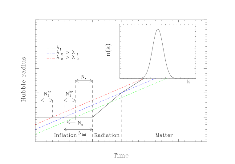
Figure 1: Sketch of the evolution of the physical size in an inflationary universe where the cosmological perturbations are placed in a non-vacuum state characterized by the distribution $n(k)$.

Interestingly enough, this number does not depend on the scale $k$ but only on the Hubble radius during inflation $H_{\rm inf}$. This means that for each scale considered separately, the back-reaction problem starts to be important after the same number of e-folds $N_{\rm e}=N^{\rm br}$ counted back from horizon exit (this is why in Fig. 1, one has $N_{1}^{\rm br}=N_{3}^{\rm br}$ for the two different scales $\lambda_{1}$ and $\lambda_{3}$). If, for instance, we consider the case where inflation takes place at GUT scales, $M_{\rm inf}\simeq 10^{16}\mbox{GeV}$, then $H_{\rm inf}\simeq 10^{13}\mbox{GeV}$ and one obtains $N^{\rm br}\simeq 7$ in agreement with the estimates of Ref. ll . If the distribution $n(k)$ is not strongly peaked around a particular scale but is rather spread over a large interval, it is clear that the important mode of the problem is, very roughly speaking, the populated smallest scale (i.e. $\simeq\lambda_{1}$ in Fig. 1). In the following, this scale is denoted by $\lambda_{\rm pop}$. The value of this scale clearly depends upon the form of the distribution $n(k)$. As it can be seen in Fig. 1, $\lambda_{\rm pop}$ is the scale for which the back-reaction problem shows up first, as we go backward in time, since the other modes with larger wavelengths have not yet penetrated deeply into the horizon and therefore do not yet face a back-reaction problem. As a consequence, this scale determines the total number of e-folds during inflation without a back-reaction problem.

Once the number $N^{\rm br}$ has been calculated, the total number of e-folds during inflation without a back-reaction problem is a priori fixed. It remains to be checked whether this number is still sufficient to solve the usual problems of the hot big bang model. We now turn to this question. Let $N_{*}(\lambda)$ be the number of e-folds, for a given scale $\lambda$, between horizon exit during inflation and the beginning of the radiation era, see Fig. 1. The total number of e-folds of inflation without a back-reaction problem is then $N_{\rm inf}\equiv N^{\rm br}+N_{*}$. The number $N_{*}$ is given by $N_{*}(\lambda)=\ln(a_{0}/a_{*})-N_{\rm r}-N_{\rm m}$, where $a_{0}$ and $a_{*}(\lambda)$ are the scale factor at present time and at first horizon crossing, respectively. The quantities $N_{\rm r}$ and $N_{\rm m}$ are the number of e-folds during the radiation and matter dominated epochs. The ratio $a_{0}/a_{*}$ is given by $(\lambda/\ell_{\rm H})H_{\rm inf}/H_{0}$, where $\ell_{{}_{\rm H}}$ is the present day Hubble radius and $H_{0}$ is the present value of the Hubble parameter given by $H_{0}/m_{{}_{\rm Pl}}\simeq 10^{-61}$. The quantities $N_{\rm r}$ and $N_{\rm m}$ are given by $N_{\rm r}=\ln(T_{\rm rh}/T_{\rm eq})$ and $N_{\rm m}\simeq\ln(z_{\rm eq})\simeq 9$. $T_{\rm rh}$ is the reheating temperature which can be expressed as $T_{\rm rh}\simeq(\Gamma m_{{}_{\rm Pl}})^{1/2}$ where $\Gamma$ is the decay width of the inflaton. For consistency, one must have $M_{\rm inf}\geq T_{\rm rh}$. $T_{\rm eq}$ is the temperature at equivalence between radiation and matter and its value reads $T_{\rm eq}\simeq 5\times 10^{-9}\mbox{GeV}\simeq 5\times 10^{-28}m_{{}_{\rm Pl}}$. The quantity $N_{*}(\lambda)$ can be expressed as

$$N_{*}(\lambda)\simeq\ln\biggl{(}\frac{\lambda}{\ell_{{}_{\rm H}}}\biggr{)}+\biggl{[}\log_{10}\biggl{(}\frac{H_{\rm inf}}{m_{{}_{\rm Pl}}}\biggr{)}-\log_{10}\biggl{(}\frac{T_{\rm rh}}{m_{{}_{\rm Pl}}}\biggr{)}+29\biggr{]}\times\ln 10\,.$$ (14)

From now on, in order to simplify the discussion, we assume that the decay width of the inflaton field is such that $T_{\rm rh}\simeq M_{\rm inf}$. Under these conditions, the usual problems are solved if the number $N_{\rm inf}$ is such that $N_{\rm inf}(\lambda_{\rm pop})\simeq\ln(\lambda_{\rm pop}/\ell_{{}_{\rm H}})+29\times\ln 10>-4+\ln z_{\rm end}$, where the quantity $z_{\rm end}$ is the redshift at which the standard evolution (hot big bang model) starts. It is linked to the reheating temperature by the relation $\log_{10}(z_{\rm end})\simeq 32+\log_{10}(T_{\rm rh}/m_{{}_{\rm Pl}})$. This gives a constraint on the scale of inflation, namely

$$\log_{10}\biggl{(}\frac{H_{\rm inf}}{m_{{}_{\rm Pl}}}\biggr{)}<2\log_{10}\biggl{(}\frac{\lambda_{\rm pop}}{{\ell_{{}_{\rm H}}}}\biggr{)}-2.5\,.$$ (15)

It is known that inflation can take place between the TeV scale and the Planck scale which amounts to $-32<\log_{10}(H_{\rm inf}/m_{{}_{\rm Pl}})<0$. We see that the constraint given by Eq. (15) is not too restrictive. In particular, if we take $\lambda_{\rm pop}=0.1\ell_{{}_{\rm H}}$ and $H_{\rm inf}=10^{13}\mbox{GeV}$, it is satisfied. However, if we decrease the scale $\lambda_{\rm pop}$, the constraint becomes more restrictive. The constraint derived in the present article appears to be less restrictive than in Ref. ll because we do not assume that all scales are populated.

Another condition must be taken into account. We have seen that the duration of inflation without a back-reaction problem is determined by the evolution of $\lambda_{\rm pop}$. However, at the time at which the back-reaction problem shows up, one must also check that all the scales of astrophysical interest today were inside the horizon so that physically meaningful initial conditions can be chosen. This property is one of the most important advantages of the inflationary scenario. If we say that the largest scale of interest today is the horizon, this condition is equivalent to

$$N_{*}(\ell_{{}_{\rm H}})<N_{*}(\lambda_{\rm pop})+N^{\rm br}\Rightarrow N^{\rm br}>\ln\biggl{(}\frac{\ell_{{}_{\rm H}}}{\lambda_{\rm pop}}\biggr{)}\,.$$ (16)

This condition is also not very restrictive, especially for large scales. As previously, the condition can be more restrictive of one wants to populate smaller scales.

Before concluding this section, a last comment is in order. What is actually shown above is that, roughly $N^{\rm br}$ e-folds before the relevant mode left the horizon, we face a back-reaction problem, as the energy density of the perturbation $\langle n(k)|\rho|n(k)\rangle$ becomes of the same order of magnitude as the background $\rho$. So, before concluding that non-vacuum initial states may or may not turn off the inflationary phase, one should calculate the back-reaction effect, i.e., extend the present framework to second order as it was done in Ref. Abramo . To our knowledge, this analysis is still to be performed. Moreover, even if we take the most pessimistic position, that is, one in which we assume that the back-reaction of the perturbations on the background energy density prevents the inflationary phase, there still exist models of inflation where the previous difficulties do not show up. Therefore, in the most pessimistic situation, there is still a hope to reconcile non-vacuum initial states with inflation. Admittedly, the price to pay is a fine-tuning of the free parameters describing inflation and/or the non-vacuum state.

III Two-point correlation function for non-vacuum initial states

III.1 General expressions

We now turn to consider the non-vacuum states for the cosmological perturbations of quantum mechanical origin. Let ${\cal D}(\sigma)$ be a domain in momentum space, such that if ${\bf k}$ is between $0$ and $\sigma$, the domain ${\cal D}(\sigma)$ is filled by $n$ quanta, while otherwise ${\cal D}$ contains nothing. Let us note that this domain is slightly different from the one considered in Ref. MRS . The state $|\Psi_{1}(\sigma,n)\rangle$ is defined by

$$|\Psi_{1}(\sigma,n)\rangle\equiv\prod_{{\bf k}\in{\cal D}(\sigma)}\frac{(c_{\bf k}^{\dagger})^{n}}{\sqrt{n!}}|0_{\bf k}\rangle\bigotimes_{{\bf p}\not\in{\cal D}(\sigma)}|0_{\bf p}\rangle=\bigotimes_{{\bf k}\in{\cal D}(\sigma)}|n_{{\bf k}}\rangle\bigotimes_{{\bf p}\not\in{\cal D}(\sigma)}|0_{\bf p}\rangle.$$ (17)

The state $|n_{{\bf k}}\rangle$ is an $n$-particle state satisfying, at conformal time $\eta=\eta_{\rm i}$: $c_{\bf k}|n_{{\bf k}}\rangle=\sqrt{n}|(n-1)_{{\bf k}}\rangle$ and $c^{{\dagger}}_{\bf k}|n_{{\bf k}}\rangle=\sqrt{n+1}|(n+1)_{{\bf k}}\rangle$. We have the following property

$$\langle\Psi_{1}(\sigma,n)|\Psi_{1}(\sigma^{\prime},n^{\prime})\rangle=\delta(\sigma-\sigma^{\prime})\delta_{nn^{\prime}}.$$ (18)

It is clear from the definition of the state $|\Psi_{1}\rangle$ that the transition between the empty and the filled modes is sharp. In order to “smooth out” the state $|\Psi_{1}\rangle$, we consider a state $|\Psi_{2}\rangle$ as a quantum superposition of $|\Psi_{1}\rangle$. In doing so, we introduce an, a priori, arbitrary function $g(\sigma;k_{\rm b})$ of $\sigma$. The definition of the state $|\Psi_{2}(n,k_{\rm b})\rangle$ is

$$|\Psi_{2}(n,k_{\rm b})\rangle\equiv\int_{0}^{+\infty}{\rm d}\sigma g(\sigma;k_{\rm b})|\Psi_{1}(\sigma,n)\rangle,$$ (19)

where $g(\sigma;k_{\rm b})$ is a given function which defines the privileged scale $k_{\rm b}$. We assume that the state is normalized and therefore $\int_{0}^{+\infty}g^{2}(\sigma;k_{\rm b}){\rm d}\sigma=1$. In the state $|\Psi_{1}(\sigma,n)\rangle$, for any domain ${\cal D}$ one has MRS :

$$\langle\Psi_{1}(\sigma,n)|c_{\bf p}c_{\bf q}|\Psi_{1}(\sigma,n)\rangle = \langle\Psi_{1}(\sigma,n)|c_{\bf p}^{{\dagger}}c_{\bf q}^{{\dagger}}|\Psi_{1}(\sigma,n)\rangle=0,$$ (20)

$$\langle\Psi_{1}(\sigma,n)|c_{\bf p}c_{\bf q}^{{\dagger}}|\Psi_{1}(\sigma,n)\rangle = n{\rm\delta}({\bf q}\in{\cal D}){\rm\delta}({\bf p}-{\bf q})+{\rm\delta}({\bf p}-{\bf q}),$$ (21)

$$\langle\Psi_{1}(\sigma,n)|c_{\bf p}^{{\dagger}}c_{\bf q}|\Psi_{1}(\sigma,n)\rangle = n{\rm\delta}({\bf q}\in{\cal D}){\rm\delta}({\bf p}-{\bf q}).$$ (22)

In these formulas, ${\rm\delta}({\bf q}\in{\cal D})$ is a function that is equal to 1 if ${\bf q}\in{\cal D}$ and 0 otherwise. These relations will be employed in the sequel for the computation of the CMB temperature anisotropies for the different non-vacuum initial states.

III.2 Two-point correlation function of the CMB temperature anisotropy

The spherical harmonic expansion of the cosmic microwave background temperature anisotropy, as a function of angular position, is given by

$$\frac{\delta T}{T}({\bf e})=\sum_{\ell m}a_{\ell m}{\cal W}_{\ell}Y_{\ell m}({\bf e})\qquad{\rm with}\qquad a_{\ell m}=\int{\rm d}\Omega_{{\bf e}}\frac{\delta T}{T}({\bf e})Y_{\ell m}^{*}({\bf e}).$$ (23)

The ${\cal W}_{\ell}$ stands for the $\ell$-dependent window function of the particular experiment. In the work presented here, we are interested in a non-Gaussian signature of primordial origin. We are thus focusing on large angular scales, for which the main contribution to the temperature anisotropy is given by the Sachs-Wolfe effect, implying

$$\frac{\delta T}{T}({\bf e})\simeq\frac{1}{3}\Phi[\eta_{\rm lss},{\bf e}(\eta_{0}-\eta_{\rm lss})],$$ (24)

where $\Phi(\eta,{\bf x})$ is the Bardeen potential, while $\eta_{0}$ and $\eta_{\rm lss}$ denote respectively the conformal times now and at the last scattering surface. Note that the previous expression is only valid for the standard Cold Dark Matter model (sCDM). In the following, we will also be interested in the case where a cosmological constant is present ($\Lambda$CDM model) since this seems to be favored by recent observations. Then, the integrated Sachs-Wolfe effect plays a non-negligible role on large scales and the expression giving the temperature fluctuations is not as simple as the previous one.

In the theory of cosmological perturbations of quantum mechanical origin, the Bardeen variable becomes an operator, and its expression can be written as MRS

$$\Phi(\eta,{\bf x})=\frac{\ell_{\rm Pl}}{\ell_{0}}\frac{3}{4\pi}\int{\rm d}{\bf k}\biggl{[}c_{\bf k}(\eta_{\rm i})f_{k}(\eta)e^{i{\bf k}\cdot{\bf x}}+c_{\bf k}^{{\dagger}}(\eta_{\rm i})f_{k}^{*}(\eta)e^{-i{\bf k}\cdot{\bf x}}\biggr{]}~{},$$ (25)

where $\ell_{\rm Pl}=(G\hbar)^{1/2}$ is the Planck length. In the following, we will consider the class of models of power-law inflation since the power spectrum of the fluctuations is then explicitly known. In this case, the scale factor reads $a(\eta)=\ell_{0}|\eta|^{1+\beta}$, where $\beta\leq-2$ is a priori a free parameter. However, in order to obtain an almost scale-invariant spectrum, $\beta$ should be close to $-2$. In the previous expression of the scale factor, the quantity $\ell_{0}$ has the dimension of a length and is equal to the Hubble radius during inflation if $\beta=-2$. The parameter $\ell_{0}$ also appears in Eq. (25). The factor $3/(4\pi)$ in that equation has been introduced for future convenience: the factor $3$ will cancel the $1/3$ in the Sachs-Wolfe formula and the factor $1/(4\pi)$ will cancel the factor $4\pi$ appearing when the complex exponentials are expressed in terms of Bessel functions and spherical harmonics. The mode function $f_{k}(\eta)$ of the Bardeen operator is related to the mode function $\mu_{k}(\eta)$ of the perturbed inflaton through the perturbed Einstein equations. In the case of power-law inflation and in the long wavelength limit, the function $f_{k}(\eta)$ is given in terms of the amplitude $A_{{}_{\rm S}}$ and the spectral index $n_{\rm s}$ of the induced density perturbations by

$$k^{3}|f_{k}|^{2}=A_{{}_{\rm S}}k^{n_{\rm s}-1}~{}.$$ (26)

Using the Rayleigh equation and the completeness relation for the spherical harmonics we have

$$\exp\biggl{[}i(\eta_{0}-\eta_{\rm lss}){\bf k}\cdot{\bf e}\biggr{]}=4\pi\sum_{\ell m}i^{\ell}j_{\ell}[k(\eta_{0}-\eta_{\rm lss})]Y_{\ell m}^{*}({\bf k})Y_{\ell m}({\bf e})~{},$$ (27)

where $j_{\ell}$ denotes the spherical Bessel function of order $\ell$. Equations (23), (24), (25) and  (27) imply

$$a_{\ell m}=\frac{\ell_{\rm Pl}}{\ell_{0}}e^{i\pi\ell/2}\int{\rm d}{\bf k}\biggl{[}c_{\bf k}(\eta_{\rm i})f_{k}(\eta)+c_{-{\bf k}}^{{\dagger}}(\eta_{\rm i})f_{k}^{*}(\eta)\biggr{]}j_{\ell}[k(\eta_{0}-\eta_{\rm lss})]Y_{\ell m}^{*}({\bf k})~{}.$$ (28)

At this point we need to somehow restrict the shape of the domain ${\cal D}$. We assume that the domain only restricts the modulus of the vectors, while it does not act on their direction. Then, from Eq. (28), one deduces

$$\langle\Psi_{1}(\sigma,n)|a_{\ell_{1}m_{1}}a_{\ell_{2}m_{2}}^{*}|\Psi_{1}(\sigma,n)\rangle = \delta_{\ell_{1}\ell_{2}}\delta_{m_{1}m_{2}}\frac{\ell_{\rm Pl}^{2}}{\ell_{0}^{2}}\int_{0}^{+\infty}\frac{{\rm d}k}{k}j_{\ell_{1}}^{2}[k(\eta_{0}-\eta_{\rm lss})]k^{3}|f_{k}|^{2}[1+2n\delta(k\in{\cal D})]$$ (29)

$$= \frac{\ell_{\rm Pl}^{2}}{\ell_{0}^{2}}\biggl{[}C_{\ell_{1}}+2nD_{\ell_{1}}^{(1)}(\sigma)\biggr{]}\delta_{\ell_{1}\ell_{2}}\delta_{m_{1}m_{2}}~{},$$

with

$$D_{\ell}^{(1)}(\sigma)\equiv\int_{0}^{\sigma}j_{\ell}^{2}[k(\eta_{0}-\eta_{\rm lss})]k^{3}|f_{k}|^{2}\frac{{\rm d}k}{k}=\frac{\pi}{2}A_{{}_{\rm S}}\int_{0}^{\sigma}J_{\ell+1/2}^{2}(k)k^{n_{\rm S}-3}{\rm d}k\equiv\frac{\pi}{2}A_{{}_{\rm S}}\bar{D}_{\ell}^{(1)}(\sigma)~{},$$ (30)

where $J_{\ell}(z)$ is an ordinary Bessel function of order $\ell$. In the last equality and in what follows we take $\eta_{0}-\eta_{\rm lss}=1$. The amplitude $A_{{}_{\rm S}}$ and the spectral index $n_{\rm s}$ are defined by Eq. (26). Thus, the multipole moments $C_{\ell}^{(1)}$, in the state $|\Psi_{1}\rangle$, are given by

$$C_{\ell}^{(1)}(\sigma)=C_{\ell}+2nD_{\ell}^{(1)}(\sigma)~{},$$ (31)

where $C_{\ell}$ is the “standard” multipole, i.e., the multipole obtained in the case where the quantum state is the vacuum, i.e., $n=0$. Let us calculate the same quantity in the state $|\Psi_{2}\rangle$. Performing a similar analysis as the above one, we find

$$\langle\Psi_{2}(n,k_{\rm b})|a_{\ell_{1}m_{1}}a_{\ell_{2}m_{2}}^{*}|\Psi_{2}(n,k_{\rm b})\rangle = \delta_{\ell_{1}\ell_{2}}\delta_{m_{1}m_{2}}\frac{\ell_{\rm Pl}^{2}}{\ell_{0}^{2}}\biggl{[}\int_{0}^{+\infty}j_{\ell_{1}}^{2}[k(\eta_{0}-\eta_{\rm lss})]k^{3}|f_{k}|^{2}\frac{{\rm d}k}{k}$$ (32)

$$+2n\int_{0}^{+\infty}{\rm d}\sigma g^{2}(\sigma;k_{\rm b})\int_{0}^{\sigma}j_{\ell_{1}}^{2}[k(\eta_{0}-\eta_{\rm lss})]k^{3}|f_{k}|^{2}\frac{{\rm d}k}{k}\biggr{]}~{}.$$

Defining $g^{2}(\sigma;k_{\rm b})\equiv{\rm d}h/{\rm d}\sigma$ [we will see below that this function $h$, actually $h(k_{\rm b})$, cannot be arbitrary] and integrating by parts leads to

$$\langle\Psi_{2}(n,k_{\rm b})|a_{\ell_{1}m_{1}}a_{\ell_{2}m_{2}}^{*}|\Psi_{2}(n,k_{\rm b})\rangle = \delta_{\ell_{1}\ell_{2}}\delta_{m_{1}m_{2}}\frac{\ell_{\rm Pl}^{2}}{\ell_{0}^{2}}\int_{0}^{+\infty}j_{\ell_{1}}^{2}[k(\eta_{0}-\eta_{\rm lss})]k^{3}|f_{k}|^{2}\biggl{\{}1+2nh(\infty)\biggl{[}1-\frac{h(k)}{h(\infty)}\biggr{]}\biggr{\}}\frac{{\rm d}k}{k}$$ (33)

$$= \frac{\ell_{\rm Pl}^{2}}{\ell_{0}^{2}}\biggl{[}C_{\ell_{1}}+2nD_{\ell_{1}}^{(2)}\biggr{]}\delta_{\ell_{1}\ell_{2}}\delta_{m_{1}m_{2}}~{},$$

with

$$D_{\ell}^{(2)}\equiv h(\infty)\int_{0}^{+\infty}j_{\ell}^{2}[k(\eta_{0}-\eta_{\rm lss})]\biggl{[}1-\frac{h(k)}{h(\infty)}\biggr{]}k^{3}|f_{k}|^{2}\frac{{\rm d}k}{k}=\frac{\pi}{2}A_{{}_{\rm S}}\int_{0}^{+\infty}J_{\ell+1/2}^{2}(k)\bar{h}(k)k^{n_{\rm S}-3}{\rm d}k\equiv\frac{\pi}{2}A_{{}_{\rm S}}\bar{D}_{\ell}^{(2)}~{},$$ (34)

where $\bar{h}(k)\equiv h(\infty)[1-h(k)/h(\infty)]$. To perform this calculation, we have not assumed anything on $h(\infty)$ or $h(0)$. We see that the relation $g^{2}(k)\equiv{\rm d}h/{\rm d}k$ requires the function $h(k)$ to be monotonically increasing with $k$. It is interesting that, already at this stage of the calculations, very stringent conditions are required on the function $h(k)$ which is therefore not arbitrary. This implies that the function $\bar{h}(k)$ which appears in the correction to the multipole moments is always positive, vanishes at infinity and is monotonically decreasing with $k$. An explicit profile for $\bar{h}(k)$ is given below. In addition, the state $|\Psi_{2}(n,k_{\rm b})\rangle$ must be normalized, which amounts to take, see Section III, $\int_{0}^{\infty}g^{2}(\sigma;k_{\rm b}){\rm d}\sigma=1$. Using the definition of the function $g^{2}$, we easily find

$$h(\infty)-h(0)=1\Rightarrow\bar{h}(0)=1.$$ (35)

The total power spectrum of the Bardeen potential can be written as

$$k^{3}|\Phi_{k}|^{2}\propto A_{{}_{\rm S}}k^{n_{\rm S}-1}\biggl{\{}1+2nh(\infty)\biggl{[}1-\frac{h(k)}{h(\infty)}\biggr{]}\biggr{\}}=A_{{}_{\rm S}}k^{n_{{}_{\rm S}}-1}[1+2n\bar{h}(k)].$$ (36)

The exact proportionality coefficient is derived below. Observations indicate that $n_{{}_{\rm S}}\simeq 1$ and for simplicity we will take $n_{{}_{\rm S}}=1$. Then, if the function $h(k)$ is chosen such that it contains a preferred scale, see the Introduction, and such that it is approximatively constant on both sides, the model becomes very similar to the one presented in Ref. lps for, in the notation of that article, $p>1$. In Ref. lps the allowed range of parameters is $0.8<p<1.7$ with an especially good agreement for the inverted step $p<1$. In our case, another difference consists in the fact that the oscillations in the spectrum studied in Ref. lps are not present due to the monotony condition on the function $h(k)$. In the following, in order to perform concrete calculations, we will choose an analytical form for $\bar{h}(k)$ which mimics the behavior of the spectrum considered in Ref. lps with $p>1$. Interestingly enough, we will see that the final result does not strongly depend on the values of the free parameters that describe the function $\bar{h}(k)$. As we have seen previously, we can write the multipole moments in the state $|\Psi_{2}\rangle$ as

$$C_{\ell}^{(2)}=C_{\ell}+2nD_{\ell}^{(2)}~{}.$$ (37)

Substituting the well-known expression for the $C_{\ell}$’s and the definition of $D_{\ell}^{(2)}$ given by Eq. (34), one finds that the coefficients $C_{\ell}^{(2)}$ are given by

$$C_{\ell}^{(2)}=A_{{}_{\rm S}}\frac{\pi}{2}\biggl{\{}{1\over 2^{3-n_{\rm s}}}{\Gamma(3-n_{\rm s})\Gamma[\ell+(n_{\rm s}-1)/2]\over\Gamma^{2}[(4-n_{\rm s})/2]\Gamma[\ell-(n_{\rm s}-5)/2]}+2n{\bar{D}_{\ell}}^{(2)}\biggr{\}}.$$ (38)

As a next step, one has to normalize the spectrum or, in other words, we need to determine the value of $A_{\rm S}$. We choose to use the value of $Q_{{\rm rms-PS}}=T_{0}[5C_{2}^{(2)}{\cal W}_{2}^{2}/(4\pi)]^{1/2}(\ell_{\rm Pl}/\ell_{0})\sim 18\mu K$ with $T_{0}=2.7K$ measured by the COBE satellite. The quadrupole is then

$$C_{2}^{(2)}=A_{{}_{\rm S}}\frac{\pi}{2}\biggl{\{}{1\over 2^{3-n_{\rm s}}}{\Gamma(3-n_{\rm s})\Gamma[2+(n_{\rm s}-1)/2]\over\Gamma^{2}[(4-n_{\rm s})/2]\Gamma[4-(n_{\rm s}-1)/2]}+2n{\bar{D}_{2}}^{(2)}\biggr{\}}\Rightarrow A_{{}_{\rm S}}=\frac{8}{5{\cal W}_{2}^{2}}\frac{Q_{\rm rms-PS}^{2}}{T_{0}^{2}}\frac{\ell_{0}^{2}}{\ell_{\rm Pl}^{2}}\biggl{[}\frac{1}{6\pi}+2n{\bar{D}_{2}}^{(2)}\biggr{]}^{-1},$$ (39)

where, in order to establish the last relation, and hereafter, we have assumed $n_{{}_{\rm S}}=1$. The measurements are often expressed in terms of band powers $\delta T_{\ell}$ defined by

$$\delta T_{\ell}=\sqrt{\frac{\ell(\ell+1)}{2\pi}\frac{\ell_{\rm Pl}^{2}}{\ell_{0}^{2}}C_{\ell}^{(2)}}~{}.$$ (40)

For $n_{{}_{\rm S}}=1$, Eq. (39) can be simplified and the band powers defined by Eq. (40) lead to

$$\delta T_{\ell}=\frac{Q_{\rm rms-PS}}{T_{0}}\frac{1}{{\cal W}_{2}}\sqrt{\frac{12}{5}}\sqrt{\frac{1+2n\pi\ell(\ell+1){\bar{D}_{\ell}}^{(2)}}{1+12n\pi{\bar{D}_{2}}^{(2)}}}~{}.$$ (41)

The $n$-dependence in the above expression is the correction due to the non-vacuum initial state. One can easily check that if $n=0$ the corresponding band powers are constant at large scales, a property which is well-known.

Finally, we calculate the two-point correlation function at zero lag in the state $|\Psi_{2}\rangle$. Using Eqs. (23), (33), (37), the second moment, $\mu_{2}$, of the distribution is given by

$$\mu_{2}\equiv\biggl{\langle}\biggl{[}\frac{\delta T}{T}({\bf e})\biggr{]}^{2}\biggr{\rangle}=\frac{\ell_{\rm Pl}^{2}}{\ell_{0}^{2}}\sum_{\ell}\frac{2\ell+1}{4\pi}C_{\ell}^{(2)}{\cal W}^{2}_{\ell}~{}.$$ (42)

Once we have reached this point, an obvious first thing to do is to check that the two-point correlation function calculated above is consistent with present observations.

III.3 Comparison with observations

Among the available observations that one can use to check the predictions of theoretical models, two are key in cosmology: the CMB anisotropy and the matter-density power spectra. Since the initial spectrum is very similar to the one considered in Ref. lps , it is clear that the multipole moments and the matter power spectrum will also be similar to the ones obtained in that article. This already guarantees that there will be no clash with the observations. Therefore, we will not study in details all the predictions that can be done from the two-point correlation function since our main purpose in this article is to calculate the non-Gaussianity which is a clear specific signature of a non vacuum state (in Ref. lps , the CMB statistics is Gaussian). Here, we just calculate the matter power spectrum to demonstrate that it fits reasonably well the available astrophysical observations for some values of the free parameters. In addition, this illustrates well the fact that, using the available observations, we can already put some constraints on the free parameters. In Ref. MRS , although the model considered was slightly different, the multipole moments were computed and shown to be in agreement with the data if the number of quanta is a few. Therefore, having given all these reasons, it seems logical to concentrate in the present article on the matter power spectrum.

III.3.1 Choice of the weight function

We first need to choose the function $h(k)$ such that it satisfies the conditions described above. A simple ansatz is

$$h(k)=A+B\tanh\biggl{(}\alpha\ln\frac{k}{k_{\rm b}}\biggr{)}~{}.$$ (43)

In this equation, $k_{\rm b}$ represents the privileged (comoving) wave-number and $\alpha$ is a parameter which controls the sharpness of the function $h(k)$. The argument of the hyperbolic tangent is expressed in terms of the logarithm of the wave-number in order to guarantee that $k\in[0,+\infty[$, see, e.g., Ref. silk . $A$ and $B$ are two coefficients that we are going to fix now. We have $h(0)=A-B$ and $h(\infty)=A+B$. Therefore, the requirement that the state be normalized translates into the condition $B=1/2$. In fact, it is easy to see that $\bar{h}(k)$ does not depend on A. The function $\bar{h}(k)$ can be written as

$$\bar{h}(k)=\frac{1}{2}\biggl{[}1-\tanh\biggl{(}\alpha\ln\frac{k}{k_{\rm b}}\biggr{)}\biggr{]}~{}.$$ (44)

We can easily check that $\bar{h}(0)=1$ and that $\bar{h}(\infty)=0$. To make the connection with the literature, note that we are not taking $a_{0}=1$ today. Rather, $a_{0}=2\ell_{\rm H}\approx 6000~{}h^{-1}{\rm Mpc}$ which implies that a preferred scale located at $0.004~{}h~{}{\rm Mpc}^{-1}$ silk corresponds to a comoving $k_{\rm b}=24$ in our case, while a preferred scale located at $0.052~{}h~{}{\rm Mpc}^{-1}$ einasto yields $k_{\rm b}=312$ in our units. In order to illustrate the different forms of the initial spectrum, the function $\bar{h}(k)$ is represented in Fig. 2.

Figure 2: The function $\bar{h}(k)$ for $\alpha=2$ (continuous line), $\alpha=5$ (dotted line) and $\alpha=10$ (dashed line).

At this point, we need to re-investigate the back-reaction problem described before but now for the two non-vacuum states $|\Psi_{1}\rangle$ and $|\Psi_{2}\rangle$. In particular, we are going to see that we can put some constraints on the free parameters only from theoretical considerations. An analogous analysis to the one performed in Section II, now for the state $|\Psi_{1}\rangle$ leads to

$$\langle\Psi_{1}|\rho|\Psi_{1}\rangle = \frac{1}{8\pi^{3}a^{4}}\int_{0}^{+\infty}\frac{{\rm d}k}{k}k^{2}[1+2n\delta({\bf k}\in{\cal D})]\biggl{[}\mu_{k}^{\prime}\mu_{k}^{\prime*}-\frac{a^{\prime}}{a}(\mu_{k}\mu_{k}^{\prime*}+\mu_{k}^{*}\mu_{k}^{\prime})+\biggl{(}\frac{a^{\prime 2}}{a^{2}}+k^{2}\biggr{)}\mu_{k}\mu_{k}^{*}\biggr{]},$$ (45)

$$\langle\Psi_{1}|p|\Psi_{1}\rangle = \frac{1}{8\pi^{3}a^{4}}\int_{0}^{+\infty}\frac{{\rm d}k}{k}k^{2}[1+2n\delta({\bf k}\in{\cal D})]\biggl{[}\mu_{k}^{\prime}\mu_{k}^{\prime*}-\frac{a^{\prime}}{a}(\mu_{k}\mu_{k}^{\prime*}+\mu_{k}^{*}\mu_{k}^{\prime})+\biggl{(}\frac{a^{\prime 2}}{a^{2}}-\frac{k^{2}}{3}\biggr{)}\mu_{k}\mu_{k}^{*}\biggr{]}.$$ (46)

Again, as in Section II, the term which is not proportional to $n$ should be subtracted since it represents the vacuum contribution. Now, for the state $|\Psi_{2}\rangle$, one gets

$$\langle\Psi_{2}|\rho|\Psi_{2}\rangle = \int_{0}^{+\infty}\int_{0}^{+\infty}{\rm d}\sigma{\rm d}\sigma^{\prime}g^{*}(\sigma)g(\sigma^{\prime})\langle\Psi_{1}(\sigma,n)|\rho|\Psi_{1}(\sigma^{\prime},n)\rangle$$ (47)

$$= \int_{0}^{+\infty}{\rm d}\sigma|g(\sigma)|^{2}\langle\Psi_{1}(\sigma,n)|\rho|\Psi_{1}(\sigma,n)\rangle,$$ (48)

where we used the fact that $\rho$ does not act on $\sigma$. In the high-frequency regime, one obtains

$$\langle\Psi_{2}|\rho|\Psi_{2}\rangle = \langle 0|\rho|0\rangle+\frac{n}{16\pi^{2}a^{4}}\int_{0}^{\infty}\sigma^{4}|g(\sigma)|^{2}{\rm d}\sigma,$$ (49)

$$\langle\Psi_{2}|p|\Psi_{2}\rangle = \langle 0|p|0\rangle+\frac{1}{3}\frac{n}{16\pi^{2}a^{4}}\int_{0}^{\infty}\sigma^{4}|g(\sigma)|^{2}{\rm d}\sigma.$$ (50)

Clearly, the equation of state is still radiation. A comparison with Sec. II also shows that the distribution of quanta is now known explicitly and is given by $n(k)=n|g(k;k_{\rm b})|^{2}k/8$. Using $|g(\sigma)|^{2}={\rm d}h/{\rm d}\sigma$, the distribution function reads

$$n(k)=\frac{\alpha n}{16}\cosh^{-2}\biggl{[}\alpha\ln\biggl{(}\frac{k}{k_{\rm b}}\biggr{)}\biggr{]}\,.$$ (51)

This function is represented in Fig. 3 for different values of the parameter $\alpha$. It is clearly peaked around the central value $k=k_{\rm b}$.

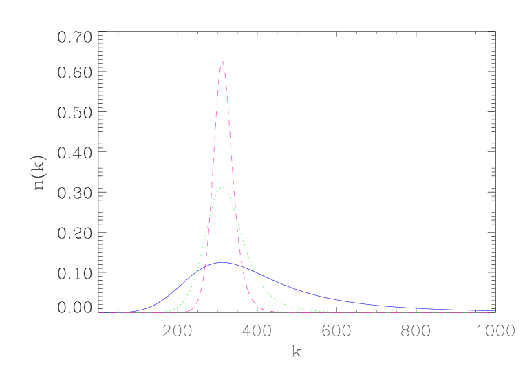
Figure 3: The function $n(k)$ for $k_{\rm b}=312$, $n=1$, $\alpha=2$ (continuous line), $\alpha=5$ (dotted line) and $\alpha=10$ (dashed line).

Finally, we end up with the following energy contribution from our state (after having removed the vacuum contribution)

$$\langle\Psi_{2}|\rho|\Psi_{2}\rangle=\frac{n}{16\pi^{2}a^{4}}\frac{\alpha}{2}\int_{0}^{\infty}\sigma^{3}\biggl{[}1-\tanh^{2}\biggl{(}\alpha\ln\frac{\sigma}{k_{\rm b}}\biggl{)}\biggr{]}{\rm d}\sigma=\frac{n}{16\pi^{2}a^{4}}\frac{k_{\rm b}^{4}}{2}\int_{-\infty}^{+\infty}\frac{e^{4v/\alpha}}{\cosh^{2}v}{\rm d}v,$$ (52)

where we have used the change of variable $v\equiv\alpha\ln(\sigma/k_{\rm b})$. Separating the integral into two pieces, it is easy to show that

$$\langle\Psi_{2}|\rho|\Psi_{2}\rangle=\frac{n}{16\pi^{2}a^{4}}k_{\rm b}^{4}\int_{0}^{\infty}\frac{\cosh(4v/\alpha)}{\cosh^{2}v}{\rm d}v=\frac{n}{16\pi^{2}a^{4}}k_{\rm b}^{4}B\biggl{(}1+\frac{2}{\alpha},1-\frac{2}{\alpha}\biggr{)}=\frac{n}{16\pi^{2}a^{4}}k_{\rm b}^{4}\Gamma\biggl{(}1+\frac{2}{\alpha}\biggr{)}\Gamma\biggl{(}1-\frac{2}{\alpha}\biggr{)},$$ (53)

where we have used Eqs. (3.512.1) and (8.384.1) of Ref. gr and where $B(x,y)\equiv\int_{0}^{1}t^{x-1}(1-t)^{y-1}{\rm d}t$ is the Euler’s integral of the first kind, see Eq. (8.380.1) of Ref. gr . In the above equation $\Gamma$ is the Euler’s integral of the second kind. These expressions are well-defined if $\alpha>2$; it is interesting to see that we can obtain constraints on the free parameters of our model just from the requirement that the energy be finite. We see in Fig. 2 that it corresponds to a situation where the function is almost a step. Repeating the same reasoning as before, we obtain the following constraint:

$$N_{\rm e}\lesssim\frac{1}{4}\biggl{\{}2\ln\biggl{(}\frac{m_{{}_{\rm Pl}}}{H_{\rm inf}}\biggr{)}-\ln n-\ln\biggr{[}\Gamma\biggl{(}1+\frac{2}{\alpha}\biggr{)}\Gamma\biggl{(}1-\frac{2}{\alpha}\biggr{)}\biggr{]}\biggr{\}}.$$ (54)

The result does not depend very much on the free parameter $n$. Roughly speaking, for the fiducial example discussed previously, the energy density of the particles becomes dominant $5$ $e$-foldings before the exit of the horizon. Since the mode considered leaves the horizon $53$ $e$-foldings before the end of inflation, we conclude that a model with $\simeq 60$ $e$-foldings does not suffer from the back-reaction problem.

In the following, we turn to the calculation of the matter power spectrum taking into account the constraint derived above, namely $\alpha>2$.

III.3.2 Calculation of the power spectrum

The first step is to calculate the two-point correlation function of the Bardeen potential. Most of the calculation has already been done in the previous subsection, see Eq. (36), but what matters now is the coefficient of proportionality which was not determined previously. One finds

$$\langle\Psi_{2}(n,k_{\rm b})|\Phi(\eta,{\bf x})\Phi(\eta,{\bf x}+{\bf r})|\Psi_{2}(n,k_{\rm b})\rangle=\frac{\ell_{\rm Pl}^{2}}{\ell_{0}^{2}}\frac{9}{4\pi}\int_{0}^{\infty}\frac{{\rm d}k}{k}\frac{\sin kr}{kr}k^{3}|f_{k}|^{2}[1+2n\bar{h}(k)].$$ (55)

The link between the power spectrum and the classical Fourier component of the Bardeen potential $\Phi(\eta,{\bf k})$, with $\Phi(\eta,{\bf x})=1/(2\pi)^{3/2}\int{\rm d}{\bf k}\Phi(\eta,{\bf k})e^{i{\bf k}\cdot{\bf x}}$, is obtained if one uses an ergodic hypothesis and identifies the “quantum” two-point correlation function with the spatial average $\langle\Phi(\eta,{\bf x})\Phi(\eta,{\bf x}+{\bf r})\rangle_{\rm V}$. In this case, one finds

$$\langle\Phi(\eta,{\bf x})\Phi(\eta,{\bf x}+{\bf r})\rangle_{\rm V}=\frac{1}{2\pi^{2}}\int_{0}^{\infty}\frac{{\rm d}k}{k}\frac{\sin kr}{kr}k^{3}|\Phi(\eta,{\bf k})|^{2}\Rightarrow\frac{1}{2\pi^{2}}k^{3}|\Phi(\eta,{\bf k})|^{2}=\frac{\ell_{\rm Pl}^{2}}{\ell_{0}^{2}}\frac{9}{4\pi}A_{{}_{\rm S}}k^{n_{\rm S}-1}[1+2n\bar{h}(k)].$$ (56)

Then, the matter power spectrum can be directly derived since the density contrast is linked to the Bardeen potential by the perturbed Einstein equations. As we mentioned above, we take $n_{{}_{\rm S}}=1$ for simplicity and get from the Poisson’s equation

$$|\delta(\eta,{\bf k})|^{2}=\frac{4}{9}\biggl{(}\frac{k_{\rm phys}}{H_{0}}\biggr{)}^{4}|\Phi(\eta,{\bf k})|^{2}\Rightarrow|\delta(\eta,{\bf k})|^{2}=\frac{\pi}{4H_{0}}\frac{\ell_{\rm Pl}^{2}}{\ell_{0}^{2}}A_{{}_{\rm S}}k_{\rm phys}[1+2n\bar{h}(k)],$$ (57)

where $A_{{}_{\rm S}}$ is the constant fixed by the COBE normalization, see Eq. (39). The quantity $\delta(\eta,{\bf k})$ in the last equations is dimensionless. The dimension-full (physical) Fourier component of the square of the density contrast is just $a_{0}^{6}$ times the previous one, $a_{0}$ being the value of the scale factor today. Defining, as usual, the spectrum $P(k)$ by $P(k)\equiv|\delta_{\rm phys}(\eta,{\bf k})|^{2}/a_{0}^{3}$ and choosing the normalization of the scale factor as $a_{0}=2\ell_{\rm H}$ where $\ell_{\rm H}$ is the Hubble radius today, one finds

$$P(k)=\frac{16\pi}{5H_{0}^{4}}\frac{Q_{\rm rms-PS}^{2}}{T_{0}^{2}}{1\over{\cal W}_{2}^{2}}\biggl{[}\frac{1}{6\pi}+2n\bar{D}_{2}^{(2)}(k_{\rm b})\biggr{]}^{-1}\biggl{[}1+2n\bar{h}(k)\biggr{]}k_{\rm phys}~{}.$$ (58)

This equation gives the initial matter power spectrum. In order to obtain the matter power spectrum today, we need to take into account the transfer function $T(k)$ which describes the evolution of the Fourier modes inside the horizon. In that case, one has

$$P(k)=T^{2}(k)\frac{16\pi}{5H_{0}^{4}}\frac{Q_{\rm rms-PS}^{2}}{T_{0}^{2}}{1\over{\cal W}_{2}^{2}}\biggl{[}\frac{1}{6\pi}+2n\bar{D}_{2}^{(2)}(k_{\rm b})\biggr{]}^{-1}\biggl{[}1+2n\bar{h}(k)\biggr{]}k_{\rm phys}~{}.$$ (59)

The sCDM transfer function is given approximatively by the following numerical fit sugiyama

$$T(k)=\frac{\ln(1+2.34q)}{2.34q}\biggl{[}1+3.89q+(16.1q)^{2}+(5.46q)^{3}+(6.71q)^{4}\biggr{]}^{-1/4},\quad q\equiv k/[(h\Gamma)\mbox{Mpc}^{-1}]~{},$$ (60)

where $\Gamma$ is the so-called shape parameter, which can be written as sugiyama

$$\Gamma\equiv\Omega_{0}he^{-\Omega_{\rm b}-\sqrt{2h}\Omega_{\rm b}/\Omega_{0}}~{},$$ (61)

where $\Omega_{0}$ is the total energy density to critical energy density ratio and $\Omega_{\rm b}$ represents the baryon contribution. More explicitly, the definitions used in this article are $\Omega_{0}=\Omega_{\rm\Lambda}+\Omega_{\rm m}=\Omega_{\rm\Lambda}+\Omega_{\rm cdm}+\Omega_{\rm b}$. We have now normalized the matter power spectrum to COBE. It is important to realize that the above procedure only works for the sCDM model since we have used the Sachs-Wolfe equation (23). The sCDM matter power spectrum is depicted in Fig. 4. The measured power spectrum of the IRAS Point Source Catalogue Redshift Survey (PSCz) pcsz has also been displayed for comparison.

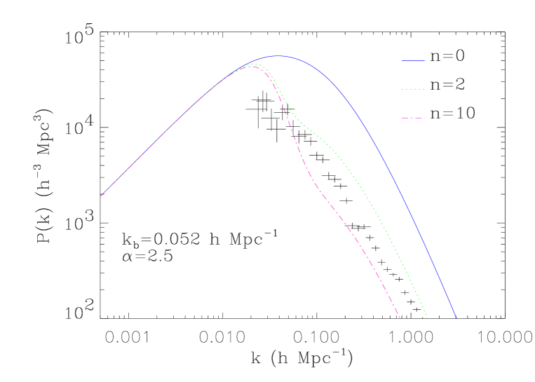
Figure 4: Matter power spectrum normalized to COBE for different numbers $n$ of quanta in the initial state. The cosmological parameters are those corresponding to the sCDM model, namely, $h=0.65$, $\Omega_{\Lambda}=0$, $\Omega_{\rm b}=0.05$, $\Omega_{\rm cdm}=0.95$ and $n_{{}_{\rm S}}=1$. The parameters describing the non vacuum state are $k_{\rm b}^{\rm phys}=0.052h\mbox{Mpc}^{-1}$ and $\alpha=2.5$. The data points represent the power spectrum measured by the PSCz survey HT .

One notices that the effect of the step in $\bar{h}(k)$ is to reduce the power at small scales which precisely improves the agreement between the theoretical curves for $n\neq 0$ and the data. Let us remind at this point that the shape of the function $\bar{h}(k)$ has not been designed for this purpose and comes from different (theoretical) reasons. Therefore, it is quite interesting to see that the power spectrum obtained from our ansatz fits reasonably well the data. This plot also confirms the result of Ref. MRS , namely that the number of quanta must be such that (for sCDM) $1\leq n<10$, i.e., cannot be too large.

Another more accurate test to check the consistency of the model with the observations is to compute the rms mass fluctuation at a scale of $r_{0}=8h^{-1}\mbox{Mpc}$. Its definition for a top hat window function reads

$$\sigma_{8}^{2}\equiv\biggl{(}\frac{\delta M}{M}\biggr{)}^{2}(r_{0}=8h^{-1}\mbox{Mpc})=\frac{1}{(4\pi r_{0}^{3}/3)^{2}}\int_{0}^{\infty}\frac{k^{3}P(k)}{2\pi^{2}}W^{2}(k)\frac{{\rm d}k}{k},$$ (62)

with

$$W(k)=4\pi r_{0}^{3}\biggl{[}\frac{\sin kr_{0}}{(kr_{0})^{3}}-\frac{\cos kr_{0}}{(kr_{0})^{2}}\biggr{]}.$$ (63)

For $n=0$ (i.e. standard sCDM model) with the following choice for the cosmological parameters, $h=0.65$, $\Omega_{0}=1$, $\Omega_{\rm b}=0.05$, a numerical calculation of the previous integral gives $\sigma_{8}\simeq 1.67$, in agreement with previous estimates, see Fig. 15 of Ref. BuW . For $h=0.5$, the result becomes $\sigma_{8}\simeq 1.28$ which is also consistent with Ref. BuW . Let us now calculate the rms mass fluctuation for $n\neq 0$. For $\alpha=2$, $k_{\rm b}^{\rm phys}=0.052h$ Mpc^-1 one finds, for our fiducial choice of the cosmological parameters, $\sigma_{8}\simeq 0.99,0.79,0.68$ for $n=1,2,3$ respectively. In the same conditions, but for $\alpha=5$, one obtains $\sigma_{8}\simeq 0.98,0.77,0.66$ which illustrates explicitly the fact that $\sigma_{8}$ is not sensitive to the parameter $\alpha$. These numbers should now be compared with those inferred from cluster abundance constraints sigma8 which give

$$\sigma_{8}^{\rm clu}=(0.5\pm 0.1)\Omega_{\rm m}^{-\gamma},$$ (64)

where $\gamma\simeq 0.5$. We recover the well-known conclusion that the $n=0$ sCDM model is ruled out because the CMB and clusters normalization are not consistent with each other (i.e. the difference is greater than $5\sigma$). On the other hand, we see that putting a few quanta improves the situation and that the $n=2$ model becomes compatible with the data at the $3\sigma$ level whereas the model $n=3$ gives the correct value at less than $2\sigma$. Fine-tuning the other cosmological parameters would allows us to achieve an even better agreement. Therefore, as announced, there exists a region in the space of parameters where the model is in agreement with the presently available data.

Now, we would like also to test the predictions of the model in the case where a cosmological constant is present. A first problem is that the value of the coefficient $A_{{}_{\rm S}}$ is no longer the same. The reason is that the integrated Sachs-Wolfe effect now plays a role at large scales and modifies the relation (24). This changes the COBE normalization and we have $C_{2}^{(2)}(\Omega_{\rm\Lambda}\neq 0)\neq C_{2}^{(2)}(\Omega_{\rm\Lambda}=0)$. As a consequence, the constant $A_{{}_{\rm S}}$ in Eq. (26) is no longer given by Eq. (39) and has to be evaluated numerically for each value of the cosmological constant. We can parameterize this dependence by introducing a coefficient $B_{{}_{\rm S}}(\Omega_{\rm\Lambda})$ such that $A_{{}_{\rm S}}(\Omega_{\rm\Lambda}\neq 0)=B_{{}_{\rm S}}(\Omega_{\rm\Lambda})A_{{}_{\rm S}}(\Omega_{\rm\Lambda}=0)$. Obviously, one has $B_{{}_{\rm S}}(\Omega_{\rm\Lambda}=0)=1$. A second problem is that the transfer function is also modified by the presence of a cosmological constant. However, the change can be easily parameterized by using a new numerical fit to the transfer function. Finally, the power spectrum can be written as

$$P(k)=T^{2}(k)\frac{g^{2}(\Omega_{0})}{g^{2}(\Omega_{\rm m})}B_{{}_{\rm S}}(\Omega_{\rm\Lambda})\frac{16\pi}{5H_{0}^{4}}\frac{Q_{\rm rms-PS}^{2}}{T_{0}^{2}}{1\over{\cal W}_{2}^{2}}\biggl{[}\frac{1}{6\pi}+2n\bar{D}_{2}^{(2)}(k_{\rm b})\biggr{]}^{-1}\biggl{[}1+2n\bar{h}(k)\biggr{]}k_{\rm phys}~{},$$ (65)

where the function $g(\Omega)$ takes into account the modification induced in the transfer function by the presence of a cosmological constant. Its expression can be written as  lewis :

$$g(\Omega)\equiv\frac{5\Omega}{2}\biggl{[}\Omega^{4/7}-\Omega_{\Lambda}+\biggl{(}1+\frac{\Omega}{2}\biggr{)}\biggl{(}1+\frac{\Omega_{\Lambda}}{70}\biggr{)}\biggr{]}^{-1}.$$ (66)

Using the previous expression, we deduce that

$$\sigma_{8}^{2}(\Omega_{0},\Omega_{\rm cdm},\Omega_{\rm b},\Omega_{\Lambda},n)=\frac{g^{2}(\Omega_{0})}{g^{2}(\Omega_{\rm m})}B_{{}_{\rm S}}(\Omega_{\Lambda})\sigma_{8}^{2}(\Omega_{0},\Omega_{\rm cdm},\Omega_{\rm b},\Omega_{\Lambda}=0,n),$$ (67)

where the last term, $\sigma_{8}^{2}(\Omega_{0},\Omega_{\rm cdm},\Omega_{\rm b},\Omega_{\Lambda}=0,n)$ does not depend explicitly on $\Omega_{\rm cdm}$ since this one does not appear in the shape parameter and therefore neither in the transfer function. Therefore, this term is equal to the value computed previously for the sCDM model. From this last equation one can easily deduce the constant $B_{{}_{\rm S}}(\Omega_{\Lambda})$, and we finally obtain

$$\sigma_{8}^{2}(\Omega_{0},\Omega_{\rm cdm},\Omega_{\rm b},\Omega_{\Lambda},n)=\frac{\sigma_{8}^{2}(\Omega_{0},\Omega_{\rm cdm},\Omega_{\rm b},\Omega_{\Lambda},n=0)}{\sigma_{8}^{2}(\Omega_{0},\Omega_{\rm cdm},\Omega_{\rm b},\Omega_{\Lambda}=0,n=0)}\sigma_{8}^{2}(\Omega_{0},\Omega_{\rm cdm},\Omega_{\rm b},\Omega_{\Lambda}=0,n).$$ (68)

The quantity $\sigma_{8}^{2}(\Omega_{0},\Omega_{\rm cdm},\Omega_{\rm b},\Omega_{\Lambda},n=0)$ is known in the literature since it is nothing but the value for the $\Lambda$CDM model. For our choice of the cosmological parameters, one has, for the $\Lambda$CDM model with $\Omega_{\rm\Lambda}=0.7$, $\sigma_{8}\simeq 1$ in agreement with Fig. 16 of Ref. BuW . The quantity $\sigma_{8}^{2}(\Omega_{0},\Omega_{\rm cdm},\Omega_{\rm b},\Omega_{\Lambda}=0,n=0)$ is the value corresponding to sCDM. Finally, the quantity $\sigma_{8}^{2}(\Omega_{0},\Omega_{\rm m},\Omega_{\rm b},\Omega_{\Lambda}=0,n)$ is known from the previous calculations. Hence, for the values of the parameters considered above, one finds $\sigma_{8}\simeq 0.59,0.47,0.40$ for $n=1,2,3$ respectively. This has to be compared with $\sigma_{8}^{\rm clu}$ which is now equal to $\sigma_{8}^{\rm clu}\simeq 0.91$ Bor ; Pier ; Rei . In this case, we see that already the first value $n=1$ gives a too small contribution. This had already been noticed in Ref. MRS for the CMB anisotropy. In this case the presence of the cosmological constant increases the height of the first acoustic peak which is also the effect of adding more and more quanta. This can result in an acoustic peak which is too high. The cure is obvious: one has to decrease the value of the cosmological constant as also noticed in Ref. lps . For instance, for $\Omega_{\Lambda}=0.5$, the value of $\sigma_{8}$ for the $\Lambda$CDM model becomes $\sigma_{8}\simeq 1.25$, see Fig. 16 of Ref. BuW . This gives for our model $\sigma_{8}\simeq 0.74,0.59,0.51$ for $n=1,2,3$ which goes in the right direction. The model with $n=1$ is now compatible at the $1.5\sigma$ level. One can decrease more the value of $\Omega_{\Lambda}$ in order to obtain a better agreement. These numbers are in full agreement with those proposed in Ref. lps where the range for the cosmological constant in a BSI model with $p>1$ was found to be $0.2<\Omega_{\rm\Lambda}<0.5$. Again, this is not surprising since we essentially deal with (almost) the same two-point correlation function.

IV Four-point correlation function for non-vacuum initial states

IV.1 General expressions

In this section we proceed with the calculation of the four-point correlation function. We first perform the calculation for the state $|\Psi_{1}\rangle$, which we then generalize for the state $|\Psi_{2}\rangle$. The first step is to establish the expression of all the combinations of four creation and/or annihilation operators taken in the state $|\Psi_{1}(\sigma,n)\rangle$. One finds

$$\langle\Psi_{1}(\sigma,n)|c_{\bf k}c_{\bf p}c_{\bf q}^{{\dagger}}c_{\bf s}^{{\dagger}}|\Psi_{1}(\sigma,n)\rangle = \biggl{[}{\rm\delta}({\bf p}-{\bf s}){\rm\delta}({\bf k}-{\bf q})+{\rm\delta}({\bf p}-{\bf q}){\rm\delta}({\bf k}-{\bf s})\biggr{]}$$ (69)

$$\times\biggl{[}1+n{\rm\delta}({\bf s}\in{\cal D})+n{\rm\delta}({\bf q}\in{\cal D})+n^{2}{\rm\delta}({\bf s}\in{\cal D}){\rm\delta}({\bf q}\in{\cal D})\biggr{]}$$

$$-n(n+1){\rm\delta}({\bf s}\in{\cal D}){\rm\delta}({\bf q}-{\bf s}){\rm\delta}({\bf p}-{\bf s}){\rm\delta}({\bf k}-{\bf q})~{},$$

$$\langle\Psi_{1}(\sigma,n)|c_{\bf k}^{{\dagger}}c_{\bf p}^{{\dagger}}c_{\bf q}c_{\bf s}|\Psi_{1}(\sigma,n)\rangle = n^{2}{\rm\delta}({\bf s}\in{\cal D}){\rm\delta}({\bf q}\in{\cal D})\biggl{[}{\rm\delta}({\bf p}-{\bf s}){\rm\delta}({\bf k}-{\bf q})+{\rm\delta}({\bf p}-{\bf q}){\rm\delta}({\bf k}-{\bf s})\biggr{]}$$ (70)

$$-n(n+1){\rm\delta}({\bf s}\in{\cal D}){\rm\delta}({\bf q}-{\bf s}){\rm\delta}({\bf p}-{\bf s}){\rm\delta}({\bf k}-{\bf q})~{},$$

$$\langle\Psi_{1}(\sigma,n)|c_{\bf k}^{{\dagger}}c_{\bf p}c_{\bf q}^{{\dagger}}c_{\bf s}|\Psi_{1}(\sigma,n)\rangle = n{\rm\delta}({\bf s}\in{\cal D}){\rm\delta}({\bf p}-{\bf q}){\rm\delta}({\bf k}-{\bf s})+n^{2}{\rm\delta}({\bf s}\in{\cal D}){\rm\delta}({\bf q}\in{\cal D}){\rm\delta}({\bf p}-{\bf q}){\rm\delta}({\bf k}-{\bf s})$$ (71)

$$+n^{2}{\rm\delta}({\bf s}\in{\cal D}){\rm\delta}({\bf p}\in{\cal D}){\rm\delta}({\bf q}-{\bf s}){\rm\delta}({\bf k}-{\bf p})$$

$$-n(n+1){\rm\delta}({\bf s}\in{\cal D}){\rm\delta}({\bf q}-{\bf s}){\rm\delta}({\bf p}-{\bf q}){\rm\delta}({\bf k}-{\bf s})~{},$$

$$\langle\Psi_{1}(\sigma,n)|c_{\bf k}c_{\bf p}^{{\dagger}}c_{\bf q}^{{\dagger}}c_{\bf s}|\Psi_{1}(\sigma,n)\rangle = n{\rm\delta}({\bf s}\in{\cal D})\biggl{[}{\rm\delta}({\bf q}-{\bf s}){\rm\delta}({\bf k}-{\bf p})+{\rm\delta}({\bf p}-{\bf s}){\rm\delta}({\bf k}-{\bf q})\biggr{]}$$ (72)

$$+n^{2}{\rm\delta}({\bf s}\in{\cal D}){\rm\delta}({\bf k}\in{\cal D})\biggl{[}{\rm\delta}({\bf q}-{\bf s}){\rm\delta}({\bf k}-{\bf p})+{\rm\delta}({\bf p}-{\bf s}){\rm\delta}({\bf k}-{\bf q})\biggr{]}$$

$$-n(n+1){\rm\delta}({\bf s}\in{\cal D}){\rm\delta}({\bf q}-{\bf s}){\rm\delta}({\bf p}-{\bf s}){\rm\delta}({\bf k}-{\bf q})~{},$$

$$\langle\Psi_{1}(\sigma,n)|c_{\bf k}^{{\dagger}}c_{\bf p}c_{\bf q}c_{\bf s}^{{\dagger}}|\Psi_{1}(\sigma,n)\rangle = +n{\rm\delta}({\bf k}\in{\cal D})\biggl{[}{\rm\delta}({\bf p}-{\bf s}){\rm\delta}({\bf k}-{\bf q})+{\rm\delta}({\bf q}-{\bf s}){\rm\delta}({\bf k}-{\bf p})\biggr{]}$$ (73)

$$+n^{2}{\rm\delta}({\bf s}\in{\cal D}){\rm\delta}({\bf k}\in{\cal D})\biggl{[}{\rm\delta}({\bf q}-{\bf s}){\rm\delta}({\bf k}-{\bf p})+{\rm\delta}({\bf p}-{\bf s}){\rm\delta}({\bf k}-{\bf q})\biggr{]}$$

$$-n(n+1){\rm\delta}({\bf s}\in{\cal D}){\rm\delta}({\bf q}-{\bf s}){\rm\delta}({\bf p}-{\bf s}){\rm\delta}({\bf k}-{\bf q})~{},$$

$$\langle\Psi_{1}(\sigma,n)|c_{\bf k}c_{\bf p}^{{\dagger}}c_{\bf q}c_{\bf s}^{{\dagger}}|\Psi_{1}(\sigma,n)\rangle = {\rm\delta}({\bf q}-{\bf s}){\rm\delta}({\bf k}-{\bf p})+n{\rm\delta}({\bf s}\in{\cal D}){\rm\delta}({\bf q}-{\bf s}){\rm\delta}({\bf k}-{\bf p})$$ (74)

$$+n{\rm\delta}({\bf q}\in{\cal D}){\rm\delta}({\bf p}-{\bf q}){\rm\delta}({\bf k}-{\bf s})+n{\rm\delta}({\bf p}\in{\cal D}){\rm\delta}({\bf q}-{\bf s}){\rm\delta}({\bf k}-{\bf p})$$

$$+n^{2}{\rm\delta}({\bf s}\in{\cal D}){\rm\delta}({\bf p}\in{\cal D})\biggl{[}{\rm\delta}({\bf q}-{\bf s}){\rm\delta}({\bf k}-{\bf p})+{\rm\delta}({\bf p}-{\bf q}){\rm\delta}({\bf k}-{\bf s})\biggr{]}$$

$$-n(n+1){\rm\delta}({\bf s}\in{\cal D}){\rm\delta}({\bf q}-{\bf s}){\rm\delta}({\bf p}-{\bf q}){\rm\delta}({\bf k}-{\bf s})~{}.$$

Then we can use the previous equations to calculate the expectation value of four coefficients $a_{\ell m}$ in the state $|\Psi_{1}(\sigma,n)\rangle$. Using Eq. (28) which links the operators $a_{\ell m}$ to the operators $c_{\bf k}$, one obtains

$$\langle\Psi_{1}(\sigma,n)|a_{\ell_{1}m_{1}}a_{\ell_{2}m_{2}}a_{\ell_{3}m_{3}}a_{\ell_{4}m_{4}}|\Psi_{1}(\sigma,n)\rangle=\frac{\ell_{\rm Pl}^{4}}{\ell_{0}^{4}}\biggl{\{}$$

$$\ \ (-1)^{m_{1}+m_{2}}\biggl{[}C_{\ell_{1}}C_{\ell_{2}}+2nC_{\ell_{1}}D_{\ell_{2}}^{(1)}+2nC_{\ell_{2}}D_{\ell_{1}}^{(1)}+4n^{2}D_{\ell_{1}}^{(1)}D_{\ell_{2}}^{(1)}\biggr{]}\delta_{\ell_{1}\ell_{3}}\delta_{\ell_{2}\ell_{4}}\delta_{m_{1},-m_{3}}\delta_{m_{2},-m_{4}}$$

$$+(-1)^{m_{1}+m_{2}}\biggl{[}C_{\ell_{1}}C_{\ell_{2}}+2nC_{\ell_{1}}D_{\ell_{2}}^{(1)}+2nC_{\ell_{2}}D_{\ell_{1}}^{(1)}+4n^{2}D_{\ell_{1}}^{(1)}D_{\ell_{2}}^{(1)}\biggr{]}\delta_{\ell_{1}\ell_{4}}\delta_{\ell_{2}\ell_{3}}\delta_{m_{1},-m_{4}}\delta_{m_{2},-m_{3}}$$

$$+(-1)^{m_{1}+m_{3}}\biggl{[}C_{\ell_{1}}C_{\ell_{3}}+2nC_{\ell_{1}}D_{\ell_{3}}^{(1)}+2nC_{\ell_{3}}D_{\ell_{1}}^{(1)}+4n^{2}D_{\ell_{1}}^{(1)}D_{\ell_{3}}^{(1)}\biggr{]}\delta_{\ell_{1}\ell_{2}}\delta_{\ell_{3}\ell_{4}}\delta_{m_{1},-m_{2}}\delta_{m_{3},-m_{4}}$$

$$-2n(n+1)E_{\ell_{1}\ell_{2}\ell_{3}\ell_{4}}^{(1)}{\cal H}_{\ell_{1}\ell_{2}\ell_{3}\ell_{4}}^{m_{1}m_{2}m_{3}m_{4}}e^{i\pi(\ell_{1}+\ell_{2}+\ell_{3}+\ell_{4})/2}\biggl{[}(-1)^{\ell_{1}+\ell_{2}+\ell_{3}+\ell_{4}}+(-1)^{\ell_{1}+\ell_{3}}+(-1)^{\ell_{2}+\ell_{3}}\biggr{]}\biggr{\}}~{},$$ (75)

with

$$E_{\ell_{1}\ell_{2}\ell_{3}\ell_{4}}^{(1)} \equiv \int_{0}^{\sigma}j_{\ell_{1}}[k(\eta_{0}-\eta_{\rm lss})]j_{\ell_{2}}[k(\eta_{0}-\eta_{\rm lss})]j_{\ell_{3}}[k(\eta_{0}-\eta_{\rm lss})]j_{\ell_{4}}[k(\eta_{0}-\eta_{\rm lss})]k^{3}|f_{k}|^{4}\frac{{\rm d}k}{k},$$ (76)

$${\cal H}_{\ell_{1}\ell_{2}\ell_{3}\ell_{4}}^{m_{1}m_{2}m_{3}m_{4}} \equiv \int{\rm d}\Omega_{{\bf e}}Y_{\ell_{1}m_{1}}^{*}(-{\bf e})Y_{\ell_{2}m_{2}}^{*}(-{\bf e})Y_{\ell_{3}m_{3}}^{*}({\bf e})Y_{\ell_{4}m_{4}}^{*}({\bf e})~{}.$$ (77)

Let us notice the following technical trick. Originally, in front of the first squared bracket in Eq. (IV.1) appears a term of the form $(-1)^{\ell_{1}+\ell_{2}}e^{i\pi(\ell_{1}+\ell_{2}+\ell_{3}+\ell_{4})/2}$. Using the fact that the presence of the Krönecker symbols implies that the corresponding expression inside the squared bracket is non vanishing only if $\ell_{1}=\ell_{3}$ and $\ell_{2}=\ell_{4}$, the previous term can be rewritten as $e^{2i\pi(\ell_{1}+\ell_{2})}=1$. This explains why it does not appear explicitly in Eq. (IV.1). Similar manipulations can be performed for the terms in front of the following two squared brackets. Let us also notice that Eq. (IV.1) includes a complex exponential factor, namely $\exp[i\pi(\ell_{1}+\ell_{2}+\ell_{3}+\ell_{4})/2]$. However, by inspection of the properties of the quantity ${\cal H}_{\ell_{1}\ell_{2}\ell_{3}\ell_{4}}^{m_{1}m_{2}m_{3}m_{4}}$, see its definition in terms of Clebsh-Gordan coefficients in the Appendix, it is possible to show that this term is in fact real. Indeed since the Clebsh-Gordan coefficients are non-vanishing only if $\ell_{1}+\ell_{2}+L=2p$ and $\ell_{3}+\ell_{4}+L=2q$ where $p,q$ are integers, we have $\ell_{1}+\ell_{2}+\ell_{3}+\ell_{4}=2(p+q-L)$, i.e., an even number. Therefore, the complex exponential factor in Eq. (IV.1) is real and equal to either $1$ or $-1$. These technical considerations will be employed in the formulas below. We also see that we now have $(-1)^{\ell_{1}+\ell_{2}+\ell_{3}+\ell_{4}}=1$. Finally, Eq. (IV.1) can be cast into a more compact form

$$\langle\Psi_{1}(\sigma,n)|a_{\ell_{1}m_{1}}a_{\ell_{2}m_{2}}a_{\ell_{3}m_{3}}a_{\ell_{4}m_{4}}|\Psi_{1}(\sigma,n)\rangle=\frac{\ell_{\rm Pl}^{4}}{\ell_{0}^{4}}\biggl{\{}(-1)^{m_{1}+m_{2}}C_{\ell_{1}}^{(1)}C_{\ell_{2}}^{(1)}\delta_{\ell_{1}\ell_{3}}\delta_{\ell_{2}\ell_{4}}\delta_{m_{1},-m_{3}}\delta_{m_{2},-m_{4}}$$

$$+(-1)^{m_{1}+m_{2}}C_{\ell_{1}}^{(1)}C_{\ell_{2}}^{(1)}\delta_{\ell_{1}\ell_{4}}\delta_{\ell_{2}\ell_{3}}\delta_{m_{1},-m_{4}}\delta_{m_{2},-m_{3}}+(-1)^{m_{1}+m_{3}}C_{\ell_{1}}^{(1)}C_{\ell_{3}}^{(1)}\delta_{\ell_{1}\ell_{2}}\delta_{\ell_{3}\ell_{4}}\delta_{m_{1},-m_{2}}\delta_{m_{3},-m_{4}}$$

$$-2n(n+1)E_{\ell_{1}\ell_{2}\ell_{3}\ell_{4}}^{(1)}{\cal H}_{\ell_{1}\ell_{2}\ell_{3}\ell_{4}}^{m_{1}m_{2}m_{3}m_{4}}e^{i\pi(\ell_{1}+\ell_{2}+\ell_{3}+\ell_{4})/2}\biggl{[}1+(-1)^{\ell_{1}+\ell_{3}}+(-1)^{\ell_{2}+\ell_{3}}\biggr{]}\biggr{\}}~{}.$$ (78)

The first part of this equation has the same structure as the corresponding well-known equation for the vacuum state. It is sufficient to replace $C_{\ell}$ with $C_{\ell}^{(1)}$ in the latter to obtain the first part of Eq. (IV.1). However, in addition, there is a non trivial term proportional to the coefficient $E_{\ell_{1}\ell_{2}\ell_{3}\ell_{4}}^{(1)}$ which cannot be guessed a priori. Obviously, for $n=0$, one recovers the standard result.

The calculation of the four-point correlation function in the state $|\Psi_{2}\rangle$ is a bit more involved. Using the fact that the operators $a_{\ell m}$ do not act on $\sigma$, one finds that the general expression is given by

$$\langle\Psi_{2}(n,k_{\rm b})|a_{\ell_{1}m_{1}}a_{\ell_{2}m_{2}}a_{\ell_{3}m_{3}}a_{\ell_{4}m_{4}}|\Psi_{2}(n,k_{\rm b})\rangle=\int_{0}^{\infty}{\rm d}\sigma g^{2}(\sigma;k_{\rm b})\langle\Psi_{1}(\sigma,n)|a_{\ell_{1}m_{1}}a_{\ell_{2}m_{2}}a_{\ell_{3}m_{3}}a_{\ell_{4}m_{4}}|\Psi_{1}(\sigma,n)\rangle.$$ (79)

The integration of terms of the type $C_{\ell_{1}}C_{\ell_{2}}$, $C_{\ell_{1}}D_{\ell_{2}}^{(1)}$ and $E_{\ell_{1}\ell_{2}\ell_{3}\ell_{4}}^{(1)}$ is easy and proceeds as before. The most difficult part is the integration of terms of the type $D_{\ell_{1}}^{(1)}D_{\ell_{2}}^{(1)}$. We find that, in the state $|\Psi_{2}\rangle$, the four-point correlation function is given by

$$\langle\Psi_{2}(n,k_{\rm b})|a_{\ell_{1}m_{1}}a_{\ell_{2}m_{2}}a_{\ell_{3}m_{3}}a_{\ell_{4}m_{4}}|\Psi_{2}(n,k_{\rm b})\rangle=\frac{\ell_{\rm Pl}^{4}}{\ell_{0}^{4}}\biggl{\{}$$

$$\ \ (-1)^{m_{1}+m_{2}}\biggl{[}C_{\ell_{1}}C_{\ell_{2}}+2nC_{\ell_{1}}D_{\ell_{2}}^{(2)}+2nC_{\ell_{2}}D_{\ell_{1}}^{(2)}+4n^{2}F_{\ell_{1}\ell_{2}}^{(2)}\biggr{]}\delta_{\ell_{1}\ell_{3}}\delta_{\ell_{2}\ell_{4}}\delta_{m_{1},-m_{3}}\delta_{m_{2},-m_{4}}$$

$$+(-1)^{m_{1}+m_{2}}\biggl{[}C_{\ell_{1}}C_{\ell_{2}}+2nC_{\ell_{1}}D_{\ell_{2}}^{(2)}+2nC_{\ell_{2}}D_{\ell_{1}}^{(2)}+4n^{2}F_{\ell_{1}\ell_{2}}^{(2)}\biggr{]}\delta_{\ell_{1}\ell_{4}}\delta_{\ell_{2}\ell_{3}}\delta_{m_{1},-m_{4}}\delta_{m_{2},-m_{3}}$$

$$+(-1)^{m_{1}+m_{3}}\biggl{[}C_{\ell_{1}}C_{\ell_{3}}+2nC_{\ell_{1}}D_{\ell_{3}}^{(2)}+2nC_{\ell_{3}}D_{\ell_{1}}^{(2)}+4n^{2}F_{\ell_{1}\ell_{3}}^{(2)}\biggr{]}\delta_{\ell_{1}\ell_{2}}\delta_{\ell_{3}\ell_{4}}\delta_{m_{1},-m_{2}}\delta_{m_{3},-m_{4}}$$

$$-2n(n+1)E_{\ell_{1}\ell_{2}\ell_{3}\ell_{4}}^{(2)}{\cal H}_{\ell_{1}\ell_{2}\ell_{3}\ell_{4}}^{m_{1}m_{2}m_{3}m_{4}}e^{i\pi(\ell_{1}+\ell_{2}+\ell_{3}+\ell_{4})/2}\biggl{[}1+(-1)^{\ell_{1}+\ell_{3}}+(-1)^{\ell_{2}+\ell_{3}}\biggr{]}\biggr{\}}~{},$$ (80)

with

$$F_{\ell_{1}\ell_{2}}^{(2)} \equiv \int_{0}^{+\infty}{\rm d}\sigma\bar{h}(\sigma)\frac{{\rm d}}{{\rm d}\sigma}\biggl{[}D_{\ell_{1}}^{(1)}D_{\ell_{2}}^{(1)}\biggr{]}=\frac{\pi^{2}}{4}A_{{}_{\rm S}}^{2}\int_{0}^{+\infty}{\rm d}\sigma\bar{h}(\sigma)\frac{{\rm d}}{{\rm d}\sigma}\biggl{[}\bar{D}_{\ell_{1}}^{(1)}\bar{D}_{\ell_{2}}^{(1)}\biggr{]}\equiv\frac{\pi^{2}}{4}A_{{}_{\rm S}}^{2}\bar{F}_{\ell_{1}\ell_{2}}^{(2)}$$ (81)

$$E_{\ell_{1}\ell_{2}\ell_{3}\ell_{4}}^{(2)} \equiv \int_{0}^{+\infty}j_{\ell_{1}}[k(\eta_{0}-\eta_{\rm lss})]j_{\ell_{2}}[k(\eta_{0}-\eta_{\rm lss})]j_{\ell_{3}}[k(\eta_{0}-\eta_{\rm lss})]j_{\ell_{4}}[k(\eta_{0}-\eta_{\rm lss})]\bar{h}(k)k^{3}|f_{k}|^{4}\frac{{\rm d}k}{k}$$ (82)

$$= \frac{\pi^{2}}{4}A_{{}_{\rm S}}^{2}\int_{0}^{+\infty}J_{\ell_{1}+1/2}(k)J_{\ell_{2}+1/2}(k)J_{\ell_{3}+1/2}(k)J_{\ell_{4}+1/2}(k)\bar{h}(k)k^{2n_{\rm S}-8}{\rm d}k\equiv\frac{\pi^{2}}{4}A_{{}_{\rm S}}^{2}\bar{E}_{\ell_{1}\ell_{2}\ell_{3}\ell_{4}}^{(2)}~{}.$$

We now see clearly the complication brought into the problem by the term $F_{\ell_{1}\ell_{2}}^{(2)}$. This term prevents us to reduce the terms within the squared brackets to the natural form $C_{\ell_{1}}^{(2)}C_{\ell_{2}}^{(2)}$ because $F_{\ell_{1}\ell_{2}}^{(2)}\neq D_{\ell_{1}}^{(2)}D_{\ell_{2}}^{(2)}$.

IV.2 Calculation of the excess kurtosis

We are now in a position to calculate the excess kurtosis. In the previous section, we have established the expression of the four-point correlation functions for the operator $a_{\ell m}$. In order to establish an analytical formula for the CMB excess kurtosis, one just needs to use the equation linking $a_{\ell m}$ and $\delta T/T$ and to play with the properties of the spherical harmonics. Explicitly, the excess kurtosis is defined as

$${\cal K}\equiv\mu_{4}-3\mu_{2}^{2}~{},$$ (83)

where the second moment has already been introduced and where the fourth moment, $\mu_{4}$, of the distribution is defined as

$$\mu_{4}=\langle K\rangle\qquad{\rm with~{}~{}}K\equiv\biggl{[}\frac{\delta T}{T}({\bf e})\biggr{]}^{4}~{}.$$ (84)

An important shortcoming of the previous definition is that the value of ${\cal K}$ depends on the normalization. It is much more convenient to work with a normalized (dimensionless) quantity. Therefore, we also define the normalized excess kurtosis as

$${\cal Q}\equiv{{\cal K}\over\mu_{2}^{2}}={\mu_{4}\over\mu_{2}^{2}}-3~{},$$ (85)

which is the one more commonly used in the literature. In what follows we work with either ${\cal K}$ or ${\cal Q}$ parameters. Thus, Eqs. (33), (IV.1) and (83) imply

$${\cal K} = \frac{\ell_{\rm Pl}^{4}}{\ell_{0}^{4}}\biggl{\{}3\frac{4n^{2}}{(4\pi)^{2}}\sum_{\ell_{1}\ell_{2}}(2\ell_{1}+1)(2\ell_{2}+1)\biggl{[}F_{\ell_{1}\ell_{2}}^{(2)}-D_{\ell_{1}}^{(2)}D_{\ell_{2}}^{(2)}\biggr{]}{\cal W}^{2}_{\ell_{1}}{\cal W}^{2}_{\ell_{2}}$$ (86)

$$-2n(n+1)\sum_{\ell_{1}m_{1}}\sum_{\ell_{2}m_{2}}\sum_{\ell_{3}m_{3}}\sum_{\ell_{4}m_{4}}E_{\ell_{1}\ell_{2}\ell_{3}\ell_{4}}^{(2)}{\cal H}_{\ell_{1}\ell_{2}\ell_{3}\ell_{4}}^{m_{1}m_{2}m_{3}m_{4}}e^{i\pi(\ell_{1}+\ell_{2}+\ell_{3}+\ell_{4})/2}\biggl{[}1+(-1)^{\ell_{1}+\ell_{3}}+(-1)^{\ell_{2}+\ell_{3}}\biggr{]}$$

$$\times{\cal W}_{\ell_{1}}{\cal W}_{\ell_{2}}{\cal W}_{\ell_{3}}{\cal W}_{\ell_{4}}Y_{\ell_{1}m_{1}}({\bf e})Y_{\ell_{2}m_{2}}({\bf e})Y_{\ell_{3}m_{3}}({\bf e})Y_{\ell_{4}m_{4}}({\bf e})\biggl{\}}~{}.$$

Let us first concentrate on the first term in the above equation. The terms $(2\ell_{1}+1)(2\ell_{2}+1)$ and $1/(4\pi)^{2}$ originate from the addition theorem of spherical harmonics

$$\sum_{m}Y_{\ell m}({\bf e})Y_{\ell m}^{*}({\bf k})=\frac{2\ell+1}{4\pi}P_{\ell}(\cos{\bf e}\cdot{\bf k})~{}.$$ (87)

The factor $3$ comes from the definition of ${\cal K}$, see Eq. (83). The fact that $F_{\ell_{1}\ell_{2}}^{(2)}\neq D_{\ell_{1}}^{(2)}D_{\ell_{2}}^{(2)}$ prevents this first term from vanishing. This is consistent with the previous considerations, as we have seen that in the absence of this condition the structure of the four-point correlation function would be similar to the one in the vacuum state, up to the term proportional to $E_{\ell_{1}\ell_{2}\ell_{3}\ell_{4}}^{(2)}$ of course. Let us now treat in more detail the second term in Eq. (86). Using again the addition theorem of spherical harmonics and the expression of a Legendre polynomial in terms of a spherical harmonic, $Y_{\ell 0}=\sqrt{(2\ell+1)/(4\pi)}P_{\ell}(\cos\theta)$, we can perform the sum over the indices $m_{i}$’s and express the corresponding factor in terms of the coefficient ${\cal H}_{\ell_{1}\ell_{2}\ell_{3}\ell_{4}}^{0000}$, and therefore in terms of Clebsh-Gordan coefficients, see the Appendix.

After some lengthy but straightforward algebra, one finds that the excess kurtosis in our class of models is finally given by

$${\cal K} = \frac{\ell_{\rm Pl}^{4}}{\ell_{0}^{4}}\biggl{\{}\frac{3n^{2}}{4\pi^{2}}\sum_{\ell_{1}\ell_{2}}(2\ell_{1}+1)(2\ell_{2}+1)\biggl{[}F_{\ell_{1}\ell_{2}}^{(2)}-D_{\ell_{1}}^{(2)}D_{\ell_{2}}^{(2)}\biggr{]}{\cal W}^{2}_{\ell_{1}}{\cal W}^{2}_{\ell_{2}}$$ (92)

$$-\frac{1}{32\pi^{3}}n(n+1)\sum_{\ell_{1}\ell_{2}\ell_{3}\ell_{4}}(2\ell_{1}+1)(2\ell_{2}+1)(2\ell_{3}+1)(2\ell_{4}+1)E_{\ell_{1}\ell_{2}\ell_{3}\ell_{4}}^{(2)}e^{i\pi(\ell_{1}+\ell_{2}+\ell_{3}+\ell_{4})/2}{\cal W}_{\ell_{1}}{\cal W}_{\ell_{2}}{\cal W}_{\ell_{3}}{\cal W}_{\ell_{4}}$$

$$\times\biggl{[}1+(-1)^{\ell_{1}+\ell_{3}}+(-1)^{\ell_{2}+\ell_{3}}\biggr{]}\sum_{L=\max(|\ell_{1}-\ell_{2}|,|\ell_{3}-\ell_{4}|)}^{L=\min(\ell_{1}+\ell_{2},\ell_{3}+\ell_{4})}(2L+1)\left(\begin{array}[]{ccc}\ell_{1}&\ell_{2}&L\\ 0&0&0\end{array}\right)^{2}\left(\begin{array}[]{ccc}\ell_{3}&\ell_{4}&L\\ 0&0&0\end{array}\right)^{2}\biggl{\}}~{}.$$

Let us emphasize that Eq. (92) is the general expression for the excess kurtosis for any non-vacuum state, since the only information we have used about the function $\bar{h}(k)$ is that it is always positive, it vanishes at infinity, and it is a monotonically decreasing function of $k$. This expression is just a pure number, and it is our main result. In the following, as we did in previous sections, we will choose an adequate ansatz for $h(k)$, namely that one from Eq. (43), and compute the excess kurtosis ${\cal K}$, as well as the normalized excess kurtosis ${\cal Q}$ defined by Eq. (85). We will then compare the calculated value for ${\cal Q}$ to the one quantified by the cosmic variance.

In an analogous way as for the definition of the second moment $\mu_{2}$ given in Eq. (42), and for future convenience, we can express the excess kurtosis in terms of its “multipole moments” ${\cal K}_{\ell_{1}\ell_{2}\ell_{3}\ell_{4}}$, as

$${\cal K}=\sum_{\ell_{1}\ell_{2}\ell_{3}\ell_{4}}{\cal W}_{\ell_{1}}{\cal W}_{\ell_{2}}{\cal W}_{\ell_{3}}{\cal W}_{\ell_{4}}{\cal K}_{\ell_{1}\ell_{2}\ell_{3}\ell_{4}}~{}.$$ (93)

Then, from Eqs. (34), (81) and (82), it is easy to establish that the moments ${\cal K}_{\ell_{1}\ell_{2}\ell_{3}\ell_{4}}$ can be put under the form

$${\cal K}_{\ell_{1}\ell_{2}\ell_{3}\ell_{4}} = \frac{\ell_{\rm Pl}^{4}}{\ell_{0}^{4}}A_{{}_{\rm S}}^{2}\biggl{\{}\frac{3n^{2}}{16}(2\ell_{1}+1)(2\ell_{2}+1)\biggl{[}\bar{F}_{\ell_{1}\ell_{2}}^{(2)}-\bar{D}_{\ell_{1}}^{(2)}\bar{D}_{\ell_{2}}^{(2)}\biggr{]}\delta_{\ell_{1}\ell_{3}}\delta_{\ell_{2}\ell_{4}}$$ (98)

$$-\frac{1}{128\pi}n(n+1)(2\ell_{1}+1)(2\ell_{2}+1)(2\ell_{3}+1)(2\ell_{4}+1)\bar{E}_{\ell_{1}\ell_{2}\ell_{3}\ell_{4}}^{(2)}(-1)^{(\ell_{1}+\ell_{2}+\ell_{3}+\ell_{4})/2}$$

$$\times\biggl{[}1+(-1)^{\ell_{1}+\ell_{3}}+(-1)^{\ell_{2}+\ell_{3}}\biggr{]}\sum_{L=\max(|\ell_{1}-\ell_{2}|,|\ell_{3}-\ell_{4}|)}^{L=\min(\ell_{1}+\ell_{2},\ell_{3}+\ell_{4})}(2L+1)\left(\begin{array}[]{ccc}\ell_{1}&\ell_{2}&L\\ 0&0&0\end{array}\right)^{2}\left(\begin{array}[]{ccc}\ell_{3}&\ell_{4}&L\\ 0&0&0\end{array}\right)^{2}\biggl{\}}~{}.$$

The last step consists in normalizing the spectrum. For that, we use the value of $A_{{}_{\rm S}}$ determined previously (in the sCDM case with non-vanishing quanta $n$ in the vacuum state). We obtain

$${\cal K}_{\ell_{1}\ell_{2}\ell_{3}\ell_{4}} = \frac{Q_{\rm rms-PS}^{4}}{T_{0}^{4}}{64\over 25}\frac{1}{{\cal W}_{2}^{4}}\left\{{1\over 2^{3-n_{\rm s}}}{\Gamma(3-n_{\rm s})\Gamma[2+(n_{\rm s}-1)/2]\over\Gamma^{2}[(4-n_{\rm s})/2]\Gamma[4-(n_{\rm s}-1)/2]}+2n{\bar{D}}_{2}^{(2)}\right\}^{-2}$$ (103)

$$\times\biggl{\{}\frac{3n^{2}}{16}(2\ell_{1}+1)(2\ell_{2}+1)\biggl{[}\bar{F}_{\ell_{1}\ell_{2}}^{(2)}-\bar{D}_{\ell_{1}}^{(2)}\bar{D}_{\ell_{2}}^{(2)}\biggr{]}\delta_{\ell_{1}\ell_{3}}\delta_{\ell_{2}\ell_{4}}-\frac{1}{128\pi}n(n+1)(2\ell_{1}+1)(2\ell_{2}+1)$$

$$\ \ \ \ \times(2\ell_{3}+1)(2\ell_{4}+1)\bar{E}_{\ell_{1}\ell_{2}\ell_{3}\ell_{4}}^{(2)}(-1)^{(\ell_{1}+\ell_{2}+\ell_{3}+\ell_{4})/2}\biggl{[}1+(-1)^{\ell_{1}+\ell_{3}}+(-1)^{\ell_{2}+\ell_{3}}\biggr{]}$$

$$\ \ \ \ \times\sum_{L=\max(|\ell_{1}-\ell_{2}|,|\ell_{3}-\ell_{4}|)}^{L=\min(\ell_{1}+\ell_{2},\ell_{3}+\ell_{4})}(2L+1)\left(\begin{array}[]{ccc}\ell_{1}&\ell_{2}&L\\ 0&0&0\end{array}\right)^{2}\left(\begin{array}[]{ccc}\ell_{3}&\ell_{4}&L\\ 0&0&0\end{array}\right)^{2}\biggl{\}}~{}.$$

In particular, we have the following expression for ${\cal K}_{\ell\ell\ell\ell}$:

$${\cal K}_{\ell\ell\ell\ell} = \frac{Q_{\rm rms-PS}^{4}}{T_{0}^{4}}{64\over 25}\frac{1}{{\cal W}_{2}^{4}}\left\{{1\over 2^{3-n_{\rm s}}}{\Gamma(3-n_{\rm s})\Gamma[2+(n_{\rm s}-1)/2]\over\Gamma^{2}[(4-n_{\rm s})/2]\Gamma[4-(n_{\rm s}-1)/2]}+2n{\bar{D}}_{2}^{(2)}\right\}^{-2}$$ (106)

$$\times\biggl{\{}\frac{3n^{2}}{16}(2\ell+1)^{2}\biggl{[}\bar{F}_{\ell\ell}^{(2)}-\bar{D}_{\ell}^{(2)}\bar{D}_{\ell}^{(2)}\biggr{]}-\frac{3}{128\pi}n(n+1)(2\ell+1)^{4}\bar{E}^{(2)}_{\ell\ell\ell\ell}\sum_{L=0}^{L=2\ell}(2L+1)\left(\begin{array}[]{ccc}\ell&\ell&L\\ 0&0&0\end{array}\right)^{4}\biggl{\}}~{}.$$

This expression for the multipole moments will be employed in the next section to estimate the overall amplitude of the non-Gaussian signal from non-vacuum states in a semi-analytical manner.

Let us end this section by signaling that the explicit expression for the normalized excess kurtosis parameter can be easily derived from the above formulas. Then, since this derivation is not especially illuminating, we prefer to jump directly to the numerical evaluation.

V Results

Having established the formal expression of the excess kurtosis, we now turn to the question of its numerical evaluation. As we are going to see, it turns out that it is not possible to calculate everything analytically for our specific ansatz. Therefore, we start with giving a detailed order-of-magnitude estimate of the excess kurtosis employing the model described above. After this, in the second subsection, we present a full numerical evaluation of ${\cal Q}$. The analytical estimate will help us in roughly understanding the full numerical results. Finally, a comparison with the cosmic variance of the excess kurtosis will tell us about the feasibility of detecting this non-Gaussian signal. Readers interested in just the final result can skip this first subsection and continue reading in section V.B.

V.1 Approximate analysis

In what follows, we estimate the order of magnitude of the expected excess kurtosis. We first study the function $\bar{D}_{\ell}^{(1)}(\sigma)$, defined in Section III as

$$\bar{D}_{\ell}^{(1)}(\sigma)\equiv\int_{0}^{\sigma}J_{\ell+1/2}^{2}(k)k^{n_{\rm S}-3}{\rm d}k~{}.$$ (107)

The plot of this function is represented in Fig. 5.

Figure 5: The function $\bar{D}_{\ell}^{(1)}(\sigma)$ versus $\sigma$ for $\ell=2$.

We can easily understand the qualitative behavior of this function. For small values of the argument, we take the first term of the Taylor expansion of the Bessel function and perform the integration exactly. The result reads

$$\bar{D}_{\ell}^{(1)}(\sigma)\simeq\frac{1}{2^{2\ell+1}(2\ell+n_{\rm S}-1)\Gamma^{2}(\ell+3/2)}\sigma^{2\ell+n_{\rm S}-1},\quad\sigma\ll 1~{}.$$ (108)

On the other hand, for large values of the argument, using Eq. (6.574.2) of Ref. gr , we obtain

$$\bar{D}_{\ell}^{(1)}(\sigma)\simeq\frac{\Gamma[3-n_{\rm S}]\Gamma[\ell+(n_{\rm S}-1)/2]}{2^{3-n_{\rm S}}\Gamma^{2}[2-n_{\rm S}/2]\Gamma[\ell+(5-n_{\rm S})/2]},\quad\sigma\gg 1~{}.$$ (109)

For $n_{\rm S}=1$, the above amounts to $\bar{D}_{\ell}^{(1)}(\sigma)\simeq 1/[\pi\ell(\ell+1)]$ which, for $\ell=2$, gives $\bar{D}_{2}^{(1)}(\sigma)\simeq 1/(6\pi)\simeq 0.053$ in agreement with Fig. 5. As a next step we want to understand the qualitative behavior of $\bar{D}_{\ell}^{(2)}$ as a function of $k_{\rm b}$ and $\ell$. Its definition, given in Section III, reads

$$\bar{D}_{\ell}^{(2)}\equiv\int_{0}^{+\infty}J_{\ell+1/2}^{2}(k)\bar{h}(k)k^{n_{\rm S}-3}{\rm d}k\simeq\int_{0}^{k_{\rm b}}J_{\ell+1/2}^{2}(k)k^{n_{\rm S}-3}{\rm d}k=\bar{D}_{\ell}^{(1)}(k_{\rm b}),$$ (110)

where we have used the fact that the behavior of $\bar{h}(k)$, especially for large value of the parameter $\alpha$, is very similar to a Heaviside function. In practice, for large $k_{\rm b}$ and for the range of angular frequencies we are interested in, we will have $k_{\rm b}\gg\ell$. In this case, $\bar{D}_{\ell}^{(2)}\simeq 1/[\pi\ell(\ell+1)]$. Let us now try to evaluate $\bar{F}_{\ell_{1}\ell_{2}}^{(2)}$ defined by

$$\bar{F}_{\ell_{1}\ell_{2}}^{(2)}\equiv\int_{0}^{+\infty}{\rm d}\sigma\bar{h}(\sigma)\frac{{\rm d}}{{\rm d}\sigma}\biggl{[}\bar{D}_{\ell_{1}}^{(1)}\bar{D}_{\ell_{2}}^{(1)}\biggr{]}.$$ (111)

Using again the fact that $\bar{h}(k)$ behaves like a step function, we find

$$\bar{F}_{\ell_{1}\ell_{2}}^{(2)}\simeq\int_{0}^{k_{\rm b}}{\rm d}\sigma\frac{{\rm d}}{{\rm d}\sigma}\biggl{[}\bar{D}_{\ell_{1}}^{(1)}\bar{D}_{\ell_{2}}^{(1)}\biggr{]}=\bar{D}_{\ell_{1}}^{(1)}(k_{\rm b})\bar{D}_{\ell_{2}}^{(1)}(k_{\rm b}).$$ (112)

The previous equations allow us to estimate the first term in Eq. (92). We find

$$\bar{F}_{\ell_{1}\ell_{2}}^{(2)}-\bar{D}_{\ell_{1}}^{(2)}\bar{D}_{\ell_{2}}^{(2)}\simeq 0~{}.$$ (113)

This conclusion rests on the approximation that the function $\bar{h}(k)$ behaves like a step function. In reality, this is of course not exactly the case. It would have been nice to find the order of magnitude of the correction in terms of the parameter $\alpha$ controlling the sharpness of the function $\bar{h}(k)$. Unfortunately, the complexity of the equations has prevented us from deriving such an estimate. This notwithstanding, we can be sure that the contribution of this first term to Eq. (92) will not be higher than that of the second term, see below.

The second term which participates to the excess kurtosis is given by the term proportional to the coefficient $E_{\ell_{1}\ell_{2}\ell_{3}\ell_{4}}^{(2)}$. Let us now study this coefficient in more detail. Its expression, using the approximate behavior of $\bar{h}(k)$, can be written as

$$\bar{E}_{\ell_{1}\ell_{2}\ell_{3}\ell_{4}}^{(2)} \equiv \int_{0}^{+\infty}J_{\ell_{1}+1/2}(k)J_{\ell_{2}+1/2}(k)J_{\ell_{3}+1/2}(k)J_{\ell_{4}+1/2}(k)\bar{h}(k)k^{2n_{\rm S}-8}{\rm d}k$$ (114)

$$\simeq \int_{0}^{k_{\rm b}}J_{\ell_{1}+1/2}(k)J_{\ell_{2}+1/2}(k)J_{\ell_{3}+1/2}(k)J_{\ell_{4}+1/2}(k)k^{2n_{\rm S}-8}{\rm d}k.$$ (115)

We have not been able to find a compact expression for this coefficient. However, it is easy to follow qualitatively its behavior. Its numerical value is maximum when the indices $\ell_{i}$’s are all equal. This is because this configuration maximizes the overlap of the first peak of the Bessel functions. Also when $\ell_{1}=\ell_{2}=\ell_{3}=\ell_{4}$ increases, the numerical value of $\bar{E}_{\ell_{1}\ell_{2}\ell_{3}\ell_{4}}^{(2)}$ decreases, because the coincidence between the four (first) peaks of the Bessel functions occurs at higher $k$, resulting in a factor $k^{2n_{\rm S}-8}$ much smaller. From these considerations, one can infer that the largest coefficient is $\bar{E}_{2222}^{(2)}$. Practically, this quantity does not depend on $k_{\rm b}$ because we always choose $k_{\rm b}\gg 5/2$ so that the upper bound of the integral can be considered to be the infinity. Numerically, one obtains

$$\bar{E}_{2222}^{(2)}=0.000094\simeq 10^{-4}.$$ (116)

This means that for all $\ell_{i}$’s we have $\bar{E}_{\ell_{1}\ell_{2}\ell_{3}\ell_{4}}^{(2)}\leq 10^{-4}$.

These semi-analytical considerations allow us to derive a rough estimate of the excess kurtosis. In the context of our approximation, this one does not depend on $k_{\rm b}$. Let us first write Eq. (92) as follows:

$${\cal K}=\frac{\ell_{\rm Pl}^{4}}{\ell_{0}^{4}}A_{{}_{\rm S}}^{2}({\cal K}_{1}+{\cal K}_{2})$$ (117)

and consider the first term. One has, as already mentioned previously,

$${\cal K}_{1}\equiv\frac{3n^{2}}{16}\sum_{\ell_{1}\ell_{2}\ell_{3}\ell_{4}}(2\ell_{1}+1)(2\ell_{2}+1)\biggl{[}\bar{F}_{\ell_{1}\ell_{2}}^{(2)}-\bar{D}_{\ell_{1}}^{(2)}\bar{D}_{\ell_{2}}^{(2)}\biggr{]}\delta_{\ell_{1}\ell_{3}}\delta_{\ell_{2}\ell_{4}}{\cal W}_{\ell_{1}}{\cal W}_{\ell_{2}}{\cal W}_{\ell_{3}}{\cal W}_{\ell_{4}}\simeq 0~{}.$$ (118)

Let us now study the second term. Since we have shown that the contribution of $\bar{E}_{2222}^{(2)}$ dominates the sum, we can very roughly estimate the excess kurtosis by retaining only this term. We have

$${\cal K}_{2} \equiv -\frac{1}{128\pi}n(n+1)\sum_{\ell_{1}\ell_{2}\ell_{3}\ell_{4}}{\cal W}_{\ell_{1}}{\cal W}_{\ell_{2}}{\cal W}_{\ell_{3}}{\cal W}_{\ell_{4}}(2\ell_{1}+1)(2\ell_{2}+1)(2\ell_{3}+1)(2\ell_{4}+1)\bar{E}_{\ell_{1}\ell_{2}\ell_{3}\ell_{4}}^{(2)}(-1)^{(\ell_{1}+\ell_{2}+\ell_{3}+\ell_{4})/2}$$ (123)

$$\times\biggl{[}1+(-1)^{\ell_{1}+\ell_{3}}+(-1)^{\ell_{2}+\ell_{3}}\biggr{]}\sum_{L=\max(|\ell_{1}-\ell_{2}|,|\ell_{3}-\ell_{4}|)}^{L=\min(\ell_{1}+\ell_{2},\ell_{3}+\ell_{4})}(2L+1)\left(\begin{array}[]{ccc}\ell_{1}&\ell_{2}&L\\ 0&0&0\end{array}\right)^{2}\left(\begin{array}[]{ccc}\ell_{3}&\ell_{4}&L\\ 0&0&0\end{array}\right)^{2}$$

$$\simeq -\frac{3\times 625}{128\pi}n(n+1)\bar{E}_{2222}^{(2)}\sum_{L=0}^{L=4}(2L+1)\left(\begin{array}[]{ccc}2&2&L\\ 0&0&0\end{array}\right)^{4},$$ (126)

where we have used the fact that ${\cal W}_{2}\simeq 1$ for the COBE window function, see below. The sum of the Clebsh-Gordan coefficients can easily be computed by noticing that

$$\left(\begin{array}[]{ccc}2&2&0\\ 0&0&0\end{array}\right)=\frac{1}{\sqrt{5}},\quad\left(\begin{array}[]{ccc}2&2&2\\ 0&0&0\end{array}\right)=-\left(\begin{array}[]{ccc}2&2&4\\ 0&0&0\end{array}\right)=-\sqrt{\frac{2}{35}},$$ (127)

the other coefficients being zero. The numerical value of the sum is $0.0857$ and we therefore reach the following result

$${\cal K}_{2}\simeq-\frac{3n(n+1)625}{128\pi}\times 0.0857\times 10^{-4}.$$ (128)

Now, to have an order of magnitude of the contribution to the kurtosis from the second term, ${\cal K}_{2}$, what remains to be done is to take into account the normalization. Using the expression of $A_{{}_{\rm S}}$ derived previously into Eq. (117) we finally find

$${\cal K}\simeq-10^{-2}\pi{n(n+1)\over(2n+1)^{2}}\times\frac{Q_{\rm rms-PS}^{4}}{T_{0}^{4}}.$$ (129)

Let us again stress that there is a non-trivial guess in this calculation that can only be justified by the full numerical calculation. The contribution of ${\cal K}_{2}$ is small, ${\cal K}_{2}\ll 1$. Since we have taken ${\cal K}_{1}\simeq 0$, this means that, in fact, we have assumed ${\cal K}_{2}\gg{\cal K}_{1}$. This has clearly be done without a proof because we were not able to derive an order of magnitude of ${\cal K}_{1}$ as a function of the sharpness parameter $\alpha$. Nevertheless, we will see that the previous estimate is quite good.

It is also very convenient to work with the normalization-independent quantity ${\cal Q}$. Recalling that with our approximations we have the second moment

$$\mu_{2}^{2}\simeq\frac{36}{25}\frac{Q_{\rm rms-PS}^{4}}{T_{0}^{4}}\biggl{[}\sum_{\ell=2}^{\ell_{\rm max}}\frac{2\ell+1}{\ell(\ell+1)}{\cal W}_{\ell}^{2}\biggr{]}^{2},$$ (130)

it is easy to show that ${\cal Q}$ ($\equiv{\cal Q}_{1}+{\cal Q}_{2}\simeq{\cal Q}_{2}$) can be written as

$${\cal Q}\simeq-0.0017{n(n+1)\over(2n+1)^{2}}.$$ (131)

In the above equation we have used the COBE-DMR window function ${\cal W}_{\ell}\simeq\exp\left[-\frac{1}{2}\ell({\ell}+1)(3.2^{\circ})^{2}\right]$, where $3.2^{\circ}$ is the dispersion of the antenna-beam profile measuring the angular response of the detector and we have chosen $\ell_{\rm max}=20$; we find that the sum in the expression for $\mu_{2}^{2}$ is equal to $\simeq 3.73$. As an example let us take $n=2$. Then we find ${\cal Q}\simeq-4.09\times 10^{-4}$. Of course this number should be considered only as an order-of-magnitude estimate. It can be easily improved if we add more terms in the calculation of the sum in the term ${\cal K}_{2}$. At this point, one should make clear that taking into account more terms does not mean that we consider the next-to-leading order of a consistent expansion. In the present context there is no small parameter to expand in. Therefore, the choice of the extra terms that we include in the sum is a bit arbitrary. However, this is not a serious problem since we know that the term $E_{\ell_{1}\ell_{2}\ell_{3}\ell_{4}}^{(2)}$ gives a contribution greater than the contribution coming from $E_{\ell_{1}^{\prime}\ell_{2}^{\prime}\ell_{3}^{\prime}\ell_{4}^{\prime}}^{(2)}$ provided that $\ell_{i}\ll\ell_{i}^{\prime},i=1\cdots 4$. In other words there is no mean to give a precise rule with regards to the terms that should be kept or not kept but there is clearly a general tendency which renders the improvement of the approximation possible (otherwise the sum would not be convergent). A good strategy to calculate the successive corrections is to proceed as follows. Suppose that we would like to calculate the sum ${\cal K}_{2}$ up to $\ell_{\rm max}$. A consistent requirement is that one should take into account all the terms $E_{\ell_{1}\ell_{2}\ell_{2}\ell_{4}}^{(2)}$ such that $\ell_{i}\leq\ell_{\rm max},i=1,\cdots 4$. For example if $\ell_{\rm max}=2$, then one should only include $E_{2222}^{(2)}$ as we did in our “leading order” calculation. The next step is to consider the case $\ell_{\rm max}=3$, i.e., we choose to take into account the terms $\bar{E}_{2233}^{(2)}$, $\bar{E}_{3333}^{(2)}$, $\bar{E}_{2333}^{(2)}$ and $\bar{E}_{2223}^{(2)}$ (of course we should also include the terms obtained by permutations of the indices $\ell_{i}$). In fact, it is easy to see that the last two terms do not give an extra contribution because the sum $\sum_{i}\ell_{i}$ is not even. For the two other terms, we find $\bar{E}_{2233}^{(2)}\simeq 0.000041$ and $\bar{E}_{3333}^{(2)}\simeq 0.000021$. After a lengthy but straightforward calculation, one can show that this gives an additional contribution equal to $-8.51\times 10^{-6}$. Therefore, a more accurate estimate of the normalized excess kurtosis is

$${\cal Q}\simeq-4.17\times 10^{-4}~{}.$$ (132)

We now turn to a full numerical computation of this quantity.

V.2 Full numerical results

In the previous section we have developed a rough idea of the amplitude of ${\cal Q}$. This gives us an estimate of the excess kurtosis parameter. However, due to the various approximations, a full numerical resolution of Eq. (85) proves essential.

Figure 6: The normalized excess kurtosis parameter ${\cal Q}$ in terms of the privileged (comoving) wave-number $k_{\rm b}$ for a particular representative set of parameters: $\alpha=5$ for the sharpness of the weight function signaling the privileged scale, and $n=2$ quanta in the non-vacuum initial state for the cosmological perturbations.

By resorting to Eq. (93) and using again the COBE-DMR window function, we can compute the value of ${\cal Q}$, valid on large angular scales. We plot the results in Fig. 6, where we show the normalized excess kurtosis ${\cal Q}$ for some particular values of the free parameters. As we see from it, ${\cal Q}\simeq-4.24\times 10^{-4}$ is an asymptotic value, provided we concentrate on the middle and big values of the built-in scale $k_{\rm b}$. This value almost exactly corresponds to the numerical estimate derived previously. In other words, the fact that the numerical estimate does not depend on $k_{\rm b}$ is confirmed by the plot, except for small values of the wave-numbers. In fact, this shows that the quantity ${\cal Q}$ does not depend very much on the free parameters. We have already established this property for $\alpha$ but this is also true for $n$ since, using the analytical estimate, we find, for $n=1$, ${\cal Q}\simeq-3.77\times 10^{-4}$ and for $n\to\infty$, ${\cal Q}\simeq-4.25\times 10^{-4}$. Since we know that this result does not depend on the details of the weight function $\bar{h}(k)$, we conclude that the asymptotic value obtained above is a generic value, at least for large values of $k_{\rm b}$. In particular, this is true for $k_{\rm b}\approx 300$ which corresponds to the built-in scale located roughly at the privileged scale in the matter power spectrum selected by the redshift surveys of Ref. einasto . Another important remark is that the excess kurtosis is found to be negative.

Let us now try to understand qualitatively the shape of the plot $Q$ vs. $k_{\rm b}$. The state that we consider, $|\Psi_{2}\rangle$, is a quantum superposition of states $|\Psi_{1}\rangle$, each one of these containing $n_{k}$ quanta for all the scales $k$ up to a given, fixed scale $\sigma$ [cf. Eq. (17)]. The “weight” given to each state $|\Psi_{1}\rangle$ is described by the function $g(k;k_{\rm b})$ that depends on the privileged scale $k_{\rm b}$. As already mentioned, for our ansatz of Eq. (43) we have $g(k;k_{\rm b})=(\alpha/2k)^{1/2}\cosh^{-1}[\alpha\ln(k/k_{\rm b})]$, which, as a function of $k$, is roughly “peaked” at $k_{\rm b}$. Then, in effect, we may approximately write

$$|\Psi_{2}(n,k_{\rm b})\rangle\simeq|\Psi_{1}(n,k_{\rm b})\rangle=\bigotimes_{{k}\in{\cal D}(k_{\rm b})}|n_{{k}}\rangle\bigotimes_{{p}\not\in{\cal D}(k_{\rm b})}|0_{p}\rangle.$$ (133)

Thus, we see that a small $k_{\rm b}$ will reduce the range of scales $k$ included in the domain ${\cal D}(k_{\rm b})$, and therefore also reduce the effective available number of quanta (of energy $k$). Given that we employed the Sachs–Wolfe formula, the excess kurtosis that we computed is only the “trace” of the non-Gaussian signal characterized by $k_{\rm b}$ left at large scales [this is also why there is no contradiction in using Eq. (24) while $k_{\rm b}$ can be large]. Let us consider two scales, say, $k_{{\rm b}1}$ and $k_{{\rm b}2}$ such that $k_{{\rm b}2}>k_{{\rm b}1}\gg 1$ (recall that we are taking $\eta_{0}-\eta_{\rm lss}=1$). It is clear that passing from $k_{{\rm b}1}$ to $k_{{\rm b}2}$ will not change the structure of the state $|\Psi_{2}\rangle$ at small scales. It will just enlarge the domain where there are quanta, leaving unmodified the large scale part. Therefore, as the excess kurtosis is essentially given by the large scale part of $|\Psi_{2}\rangle$, it must be independent of $k_{\rm b}$ provided that $k_{\rm b}$ is large, exactly as we find. On the other hand, if $k_{\rm b}$ is small, a change in this scale affects the structure of the state at scales that are relevant for the Sachs-Wolfe effect. As we saw previously, in this regime, the number of quanta corresponding to large scales decreases as $k_{\rm b}$ goes to zero. The result is that the excess kurtosis, whose value is directly dependent on the number of quanta, should diminish proportionally as $k_{\rm b}$ goes to zero, and this is in fact what we see in Fig. 6.

These considerations give an intuitive understanding of the main result of this article. We will see in the next section that the theoretical uncertainties on ${\cal Q}$ (as given by the cosmic variance) are roughly equal to ${\cal Q}_{{}_{\rm CV}}\simeq 1$ implying that the non-Gaussian feature studied previously would be undetectable.

V.3 Comparison with the cosmic variance

The cosmic variance quantifies the theoretical error coming from the fact that, in cosmology, observers have only access to one realization of the $\delta T/T$ stochastic process whereas theoretical predictions are expressed through ensemble averages. To compute the cosmic variance of a given quantity, say $e$, one should proceed as follows Grishchuk-Martin ; GaMa . Firstly, one has to introduce a class of unbiased estimators $\hat{E}$ of the quantity $e$, i.e., $\langle\hat{E}\rangle=e$, where in the present context the average symbol means a quantum average in the considered state. Secondly, one should compute the variance of these estimators and find the smallest one under the constraint that the estimators are unbiased. The estimator which possesses the minimal variance is the best unbiased estimator of the quantity $e$. We denote it as $\hat{E}_{\rm best}$. Finally, one should compute the variance of the best estimator $\sigma_{\hat{E}_{\rm best}}$ which is, by definition, the cosmic variance. If $\sigma_{\hat{E}_{\rm best}}=0$, then each realization gives $e$ and from one realization we can measure the quantity we are interested in. If $\sigma_{\hat{E}_{\rm best}}\neq 0$, which is obviously the usual case, one can attach a theoretical error to the quantity we seek. Let $e_{\rm real}$ be (the numerical value of) one realization of the corresponding stochastic process, then we can say that the quantity $e$ is found to be $e_{\rm real}\pm\sigma_{\hat{E}_{\rm best}}$. So far, this strategy has been successfully applied to quantities related to the two-point correlation function Grishchuk-Martin and to the three-point correlation function GaMa , in the vacuum state.

The normalized excess kurtosis is defined in Eq. (85). We see that, in the present context, we face two important complications. The first one is that one has to perform the minimization in a non-vacuum state. Let us notice in passing that this implies that the cosmic variance of the multipole moments is probably not given by the usual expression if the quantum state is no longer the vacuum. The second complication is that, in order to determine the best estimator of the normalized excess kurtosis, one has to deal with the ratio of two stochastic processes. Suppose that we want to find the best estimator of the quantity $e=e_{1}/e_{2}$ knowing the best estimators of the quantities $e_{1}$ and $e_{2}$, $\hat{E}_{\rm best}(e_{1})$ and $\hat{E}_{\rm best}(e_{2})$, respectively. The problem is that $\hat{E}_{\rm best}(e_{1}/e_{2})\neq\hat{E}_{\rm best}(e_{1})/\hat{E}_{\rm best}(e_{2})$. In this case, the calculation of the best estimator becomes much more complicated.

Therefore, the full calculation of the best estimator of the normalized excess kurtosis is a project beyond the scope of the present work and we will instead limit ourselves to an order-of-magnitude estimate of the theoretical uncertainties. This will yield a roughly correct estimate of the uncertainties without the complications of much more cumbersome analysis.

To avoid the first complication, we estimate the variance of the excess kurtosis as if it were issued from a Gaussian process, i.e., as if the quantum state were the vacuum state. To deal with the second complication, we use the following procedure. The excess kurtosis ${\cal K}$ (or its normalized version ${\cal Q}$) is just related to the fourth moment $\mu_{4}$ of the distribution from which we substract the Gaussian part $\mu_{4}^{\rm(Gauss)}=3\mu_{2}^{2}$. We will only take into account the contribution to the cosmic variance related to the fourth moment $\mu_{4}$. This last one is determined in the standard manner: the quantity $K$, defined in Eq. (84), is an unbiased estimator of $\mu_{4}$; let $\sigma_{{}_{\rm CV}}$ be its variance (in order to compute this variance one needs to calculate the eight-point correlation functions of the relevant creation and annihilation operators in the vacuum state–according to our trick to avoid the first complication, see above–) and let $\mu_{4}^{\rm real}=\langle K\rangle^{\rm real}$ be one realization of the stochastic process $K$; as it is $\sigma_{{}_{\rm CV}}$ what attaches theoretical error bars to the actual value for the mean kurtosis, we can heuristically express the effect of $\sigma_{{}_{\rm CV}}$ on $\mu_{4}$ as follows: $\mu_{4}\simeq\mu_{4}^{\rm real}\pm\sigma_{{}_{\rm CV}}$, at one sigma level. Having specified the cosmic variance of the kurtosis, we now need to relate it to the cosmic variance of the excess kurtosis. The effect of the cosmic variance is that, instead of finding the value ${\cal Q}=0$ for a Gaussian process in the vacuum state, we typically obtain a value shifted by $\pm{\cal Q}_{{}_{\rm CV}}$ which can be estimated as

$${\cal Q}_{{}_{\rm CV}}\simeq{\mu_{4}^{\rm real}-3\mu_{2}^{2}\over\mu_{2}^{2}}\simeq{\mu_{4}-3\mu_{2}^{2}\over\mu_{2}^{2}}\pm\frac{\sigma_{{}_{\rm CV}}}{\mu_{2}^{2}}=\pm\frac{\sigma_{{}_{\rm CV}}}{\mu_{2}^{2}},$$ (134)

where in the last equality, and as we mentioned above, we used the fact that the process is Gaussian. In other words, Eq. (134) shows that ${\cal Q}_{{}_{\rm CV}}$ is the normalized excess kurtosis parameter (assuming Gaussian statistics) purely due to the cosmic variance. ${\cal Q}_{{}_{\rm CV}}$ is in general non-zero sv and its magnitude increases with the theoretical uncertainty $\sigma_{{}_{\rm CV}}$.

Figure 7: The normalized excess kurtosis parameter ${\cal Q}_{{}_{\rm CV}}$ due to the cosmic variance, in the mildly non-Gaussian approximation and as function of the scalar spectral index $n_{\rm s}$. We have checked that, of the two terms in Eq. (135), it is in fact the first one (with pre-factor 72) the one that dominates the full result for ${\cal Q}_{{}_{\rm CV}}$. It is this first term what we plot in the figure for the COBE-DMR window function, including the quadrupole and for $\ell_{\rm max}=20$. The addition of the term with pre-factor 24 raises the points no more than a 5% for all values of $n_{\rm S}$.

This gives a fundamental threshold that must be overcome by any measurable excess kurtosis parameter. The expression for ${\cal Q}_{{}_{\rm CV}}$ is straightforward to obtain, although after a somewhat long algebra. It was computed in Ref. cv and gives

$${\cal Q}_{{}_{\rm CV}}=\left\{\,72\,{\sum_{\ell}(2\ell+1){C}_{\ell}^{2}{\cal W}_{\ell}^{4}\over[\sum_{\ell}(2\ell+1){C}_{\ell}{\cal W}_{\ell}^{2}]^{2}}\right.$$ (135)

$$+\,\left.24\frac{\bigl{(}\prod_{i=1}^{4}\sum_{\ell_{i}}\sum_{m_{i}=-\ell_{i}}^{\ell_{i}}{C}_{\ell_{i}}{\cal W}_{\ell_{i}}^{2}\bigr{)}\bigl{(}\sum_{L}4\pi\,\bar{\cal H}_{\ell_{1},\,\,\ell_{2}\,,\,\,\,\,L}^{m_{1},m_{2},m_{3}+m_{4}}\bar{\cal H}_{\ell_{3},\,\,\ell_{4}\,,\,\,\,\,\,\,L}^{m_{3},m_{4},-m_{3}-m_{4}}\bigl{)}^{2}}{[\sum_{\ell}(2\ell+1){C}_{\ell}{\cal W}_{\ell}^{2}]^{4}}\right\}^{1/2}.$$

As is the case for ${\cal Q}$, one of the advantages of the previous expression for ${\cal Q}_{{}_{\rm CV}}$ is that it is transparent to any particular normalization of the spectrum. We have computed the value for ${\cal Q}_{{}_{\rm CV}}$ for the COBE-DMR window function and found a value of order one for values of the scalar spectral index close to one. For illustrative purposes, we show in Fig. 7 the variation with spectral index of ${\cal Q}_{{}_{\rm CV}}$ when the term with pre-factor 24 is absent [just a 5% off of the full result]. Note that in an analogous calculation in Ref. cv the quadrupole was subtracted from the sum. The fact of including it now only increases slightly the final value for ${\cal Q}_{{}_{\rm CV}}$, showing the big contribution of the low order multipoles to the cosmic variance, as already noted in that paper.

VI Conclusions

In this article, we have presented evidence that Gaussianity is a robust property of inflation. We have seen that a departure from the standard vacuum initial conditions for the cosmological perturbations leads generically to a clear non-Gaussian signature, viz. the excess kurtosis of the CMB temperature anisotropies. The signal-to-noise ratio for the dimensionless excess kurtosis parameter is found to be

$$\biggl{|}\frac{S}{N}\biggr{|}\simeq 4\times 10^{-4},$$ (136)

and so the signal lies well below the cosmic variance and far away from experimental detection. We have found that this value is quite independent of the free parameters of the model. We have also shown that the excess kurtosis is generically negative. The only possible loophole in the argument presented above, and that we have discussed at length, is the uncertainty related to back-reaction. This issue is generically important for the inflationary phase, and one could well conceive that it could modify the evolution of the background in such a way as to increase the ratio $S/N$. However, we do not think at present one such positive conspiracy would take place, and therefore primordial Gaussianity keeps on being a generic property of single field inflationary models.

Finally, a comment is in order on the trans-Planckian problem of inflation. As already mentioned, it has been recently suggested in Ref. Chu ; HKi that trans-Planckian physics could be mimicked by a non-vacuum state (rather than by a change in the dispersion relation) implying that non-Gaussianity would be a possible observable signature of the physics on lengths much smaller than the Planck length. Unfortunately, what has been shown in the present paper for the CMB excess kurtosis leads us to conclude with a no-go conjecture: these aforementioned signatures of trans-Planckian physics will most probably be astrophysically unobservable.

Appendix

We review here some definitions and properties of quantities involving Wigner 3-$j$ symbols which are useful for the main text. We define the integral of four spherical harmonics as

$$\bar{\cal H}_{\ell_{1}\ell_{2}\ell_{3}\ell_{4}}^{m_{1}m_{2}m_{3}m_{4}} \equiv \int{\rm d}\Omega_{{\bf e}}Y_{\ell_{1}m_{1}}({\bf e})Y_{\ell_{2}m_{2}}({\bf e})Y_{\ell_{3}m_{3}}({\bf e})Y_{\ell_{4}m_{4}}({\bf e})$$ (137)

$$= (-)^{m_{3}+m_{4}}\sum_{L}\bar{\cal H}_{\ell_{1},\,\ell_{2},\,L}^{m_{1},\,m_{2},\,m_{3}+m_{4}}\bar{\cal H}_{\ell_{3},\,\ell_{4},\,L}^{m_{3},\,m_{4},\,-(m_{3}+m_{4})}~{},$$ (138)

where, following the notation of Ref. ga94 ; mo95 ; GaMa , we wrote

$$\bar{\cal H}_{\ell_{1},\,\ell_{2},\,\ell_{3}}^{m_{1},\,m_{2},\,m_{3}}\equiv\bar{\cal H}_{\ell_{1}\ell_{2}\ell_{3}}^{m_{1}m_{2}m_{3}}\equiv\int d\Omega_{\bf e}Y_{\ell_{1}}^{m_{1}}({\bf e})Y_{\ell_{2}}^{m_{2}}({\bf e})Y_{\ell_{3}}^{m_{3}}({\bf e})~{}.$$ (139)

$\bar{\cal H}_{\ell_{1}\ell_{2}\ell_{3}}^{m_{1}m_{2}m_{3}}$ has the following simple expression in terms of Wigner 3-$j$ symbols me76 :

$$\bar{\cal H}_{\ell_{1}\ell_{2}\ell_{3}}^{m_{1}m_{2}m_{3}}=\sqrt{\frac{(2\ell_{1}+1)(2\ell_{2}+1)(2\ell_{3}+1)}{4\pi}}\left(\begin{array}[]{ccc}\ell_{1}&\ell_{2}&\ell_{3}\\ 0&0&0\end{array}\right)\left(\begin{array}[]{ccc}\ell_{1}&\ell_{2}&\ell_{3}\\ m_{1}&m_{2}&m_{3}\end{array}\right).$$ (140)

In the main text we employed the quantity ${\cal H}_{\ell_{1}\ell_{2}\ell_{3}\ell_{4}}^{m_{1}m_{2}m_{3}m_{4}}$ which is simply related to $\bar{\cal H}_{\ell_{1}\ell_{2}\ell_{3}\ell_{4}}^{m_{1}m_{2}m_{3}m_{4}}$ defined above by

$${\cal H}_{\ell_{1}\ell_{2}\ell_{3}\ell_{4}}^{m_{1}m_{2}m_{3}m_{4}}=(-)^{\ell_{1}+\ell_{2}}\,\,[\bar{\cal H}_{\ell_{1}\ell_{2}\ell_{3}\ell_{4}}^{m_{1}m_{2}m_{3}m_{4}}]^{*}=(-)^{\ell_{1}+\ell_{2}}\,\,\bar{\cal H}_{\ell_{1}\ell_{2}\ell_{3}\ell_{4}}^{m_{1}m_{2}m_{3}m_{4}}~{}.$$ (141)

The last equality holds since the 3-$j$ symbols, as well as the Clebsh-Gordan coefficients, are all real.

References

- (1) R. Durrer, Journal of Physical Studies, (2002), astro-ph/0109522; W. Hu and S. Dodelson, Ann. Rev. Astron. Astrophys., (2002), astro-ph/0110414.
- (2) See, e.g., http://map.gsfc.nasa.gov/ and http://astro.estec.esa.nl/Planck/ .
- (3) J. H. P. Wu et al., Phys. Rev. Lett. 87, 251303 (2001), astro-ph/0104248; E. Komatsu et al., submitted to Astrophys. J., astro-ph/0107605 ; M. G. Santos et al., astro-ph/0107588.
- (4) M. Kunz et al. to be published in Astrophys. J. Lett., astro-ph/0111250.
- (5) G. Polenta et al., astro-ph/0201133.
- (6) L. P. Grishchuk and J. Martin, Phys. Rev. D56, 1924 (1997), gr-qc/9702018.
- (7) J. Lesgourgues, D. Polarski, A. A. Starobinsky, Nucl. Phys. B 497, 479 (1997), astro-ph/9711139.
- (8) J. Martin, A. Riazuelo and M. Sakellariadou, Phys. Rev. D 61, 083518 (2000), astro-ph/9904167.
- (9) D. Boyanovsky, F. J. Cao, H. J. de Vega, astro-ph/0102474.
- (10) C. R. Contaldi, R. Bean and J. Magueijo, Phys. Lett. B468, 189 (1999), astro-ph/9910309.
- (11) A. Linde and V. Mukhanov, Phys. Rev. D56, 535 (1997), astro-ph/9610219.
- (12) N. Bartolo, S. Matarrese and A. Riotto, astro-ph/0112261.
- (13) A. R. Liddle, D. H. Lyth, Phys. Reports 231, 1 (1993), astro-ph/9303019.
- (14) L. R. W. Abramo, R. H. Brandenberger and V. Mukhanov, Phys. Rev. D56, 3248 (1997), gr-qc/9704037; V. Mukhanov, L. R. W. Abramo and R. H. Brandenberger, Phys. Rev. Lett. 78, 1624 (1997), gr-qc/9609026.
- (15) W. Unruh, astro-ph/9802323.
- (16) J. Martin and R. H. Brandenberger, Phys. Rev. D63, 123501 (2000), hep-th/0005209; R. H. Brandenberger and J. Martin, Mod. Phys. Lett. A16, 999 (2001), astro-ph/0005432; J. Niemeyer, Phys. Rev. D63, 123502 (2000), astro-th/0005533; M. Lemoine, M. Lubo, J. Martin and J. P. Uzan, Phys. Rev. D64, 043508 (2001), hep-th/0109128; R. H. Brandenberger, S. E. Joras and J. Martin, hep-th/0112122.
- (17) R. Easther, B. R. Greene, W. H. Kinney and G. Shiu, Phys. Rev. D64, 103502 (2001), hep-th/0011241; R. Easther, B. R. Greene, W. H. Kinney and G. Shiu, hep-th/0110226.
- (18) L. Hui and W. H. Kinney, astro-ph/0109107.
- (19) P. G. Ferreira, J. Magueijo and J. Silk, Phys. Rev. D56, 4592 (1997), astro-ph/9704261.
- (20) P. G. Ferreira, J. Magueijo, and K. M. Gorski, Astrophys. J. 503, L1 (1998), astro-ph/9803256; A. F. Heavens, Mon. Not. R. Astron. Soc. 299, 805 (1998), astro-ph/9804222; D. Spergel and D. Goldberg, Phys. Rev. D 59, 103001 (1999), astro-ph/9811252; D. Goldberg and D. Spergel, Phys.Rev. D 59, 103002 (1999), astro-ph/9811251; L. Verde, L. Wang, A. Heavens and M. Kamionkowski, Mon. Not. R. Astron. Soc. 313, L141 (2000), astro-ph/9906301; A. Cooray and W. Hu, Astrophys. J. 534, 533 (2000), astro-ph/9910397; A. Gangui and J. Martin, Mon. Not. R. Astron. Soc. 313, 323 (2000), astro-ph/9908009; A. Gangui and J. Martin, Phys. Rev. D62, 103004 (2000), astro-ph/0001361; E. Komatsu and D. Spergel, Phys. Rev. D63, 063002 (2001), astro-ph/0005036; A. Gangui, L. Pogosian, and S. Winitzki, Phys. Rev. D64, 043001 (2001), astro-ph/0101453.
- (21) O. Forni and N. Aghanim, astro-ph/9905125.
- (22) N. Aghanim and O. Forni, astro-ph/9905124.
- (23) P. de Bernardis et al., Nature 404, 955 (2000), astro-ph/0004404.
- (24) S. Hanany et al., Astrophys. J. 545, L5 (2000), astro-ph/0005123.
- (25) C. Pryke et al., astro-ph/0104490; N. W. Halverson, astro-ph/0104489.
- (26) J. Adams, B. Cresswell, R. Easther, Phys. Rev. D64 123514 (2001), astro-ph/0102236.
- (27) J. Einasto et al., Nature 385, 139 (1997), astro-ph/9701018; J. A. Peacock, Mon. Not. R. Astron. Soc. 284, 885 (1997); T. J. Broadhurst et al., Nature 343, 726 (1990).
- (28) A. Zandivarez, M. G. Abadi and D. García Lambas, astro-ph/0103378.
- (29) F. Hoyle et al., astro-ph/0102163.
- (30) B. F. Roukema, G. A. Mamon and S. Bajtlik, Astron. Astrophys. 382, 397 (2002), astro-ph/0106135.
- (31) S. M. Croom et al., astro-ph/0012375.
- (32) L. M. Griffiths, J. Silk and S. Zaroubi, Mon. Not. R. Astron. Soc. 324, 712 (2001), astro-ph/0010571.
- (33) S. Landau and A. Gangui, in preparation.
- (34) A. Gangui and L. Perivolaropoulos, Astrophys. J. 447, 1 (1995), astro-ph/9408034.
- (35) V. F. Mukhanov, H. A. Feldman and R. H. Brandenberger, Phys. Rep. 215, 203 (1995).
- (36) J. Martin and D. J. Schwarz, Phys. Rev. D57, 3302 (1998), gr-qc/9704049.
- (37) L. P. Grishchuk, Phys. Rev. D57, 7154 (1994), gr-qc/9405059.
- (38) N. D. Birrell and P. C. W. Davis, “Quantum fields in curved space, Cambridge university press (1982).
- (39) I. S. Gradshteyn, I. M. Ryzhik, “Table of Integrals, Series, and Products”, Sixth edition (2000), Academic Press.
- (40) N. Sugiyama, Astrophys. J. Suppl. 100, 281 (1995).
- (41) W. Saunders et al., Mon. Not. R. Astron. Soc. 317, 55 (2000), astro-ph/0001117.
- (42) A. J. S. Hamilton and M. Tegmark, astro-ph/0008392.
- (43) E. F. Bunn and M. White, Astrophys. J. 480, 6 (1997), astro-ph/9607060.
- (44) L. Wang and P. J. Steinhardt, Astrophys. J. 508, 483 (1998), astro-ph/9804015.
- (45) S. Carroll et al., Ann. Rev. Astron. Astrophys. 30, 499 (1992).
- (46) S. Borgani et al., astro-ph/0106428.
- (47) E. Pierpaoli et al., Mon. Not. R. Astron. Soc. 325, 77 (2001), astro-ph/0010039.
- (48) T. H. Reiprich and H. Boehringer, astro-ph/0111285.
- (49) R. Scaramella, N. Vittorio, Astrophys. J.375, 439 (1991); M. Srednicki , Astrophys. J. 416, L1 (1993).
- (50) A. Gangui, F. Lucchin, S. Matarrese and S. Mollerach, Astrophys. J. 430, 447 (1994), astro-ph/9312033.
- (51) S. Mollerach, A. Gangui, F. Lucchin and S. Matarrese, Astrophys. J. 453, 1 (1995), astro-ph/9503115.
- (52) A. Gangui and J. Martin, in Ref. sht .
- (53) A. Messiah, Quantum Mechanics, Vol.2 (Amsterdam: North–Holland, 1976).