On The Spectral Energy Dependence of Gamma-Ray Burst Variability

Abstract

The variable activity of a $\gamma$-ray burst (GRB) source is thought to be correlated with its absolute peak luminosity - a relation that, if confirmed, can be used to derive an independent estimate of the redshift of a GRB. We find that bursts with highly variable light curves have greater $\nu F_{\nu}$ spectral peak energies, when we transform these energies to the cosmological rest frame using the redshift estimates derived either from optical spectral features or from the luminosity-variability distance indicator itself. This positive correlation between peak energy and variability spans $\approx$ 2 orders of magnitude and appears to accommodate GRB 980425, lending credibility to the association of this burst with SN 1998bw. The existence of such a correlation not only provides an interesting clue to the nature of this luminosity indicator but potentially reinforces the validity of the redshift estimates derived from this method. It also implies that the rest frame GRB peak energy is correlated with the intrinsic luminosity of the burst, as has been suggested in the past as an explanation of the observed hardness-intensity correlation in GRBs.

1. Introduction

Until a few years ago, gamma-ray bursts (GRBs) were known only as brief, intense flashes of high-energy radiation, with no observable traces at other wavelengths. The study of fading afterglows has enabled the measurement of redshift distances and the identification of host galaxies, establishing that GRBs are extremely luminous events detectable to much larger distances than quasars or galaxies. Consequently, GRBs can provide novel information about early epochs in the history of the universe.

Present distance estimates - which rely on optical line features in the afterglow spectrum or emission lines in the spectrum of the host galaxy - are relatively rare. There are now $\sim 20$ GRBs with optical spectroscopic redshifts (all in the range 0.43 $\leq\,z\,\leq$ 4.5). Hence, until recently it appeared that using GRBs to map the high-$z$ universe would have to wait for dedicated localization and follow-up programs like Swift and NGST. However, the discovery of two recent correlations between the degree of variability of the $\gamma$-ray light curve and the GRB luminosity (Ramirez-Ruiz & Fenimore 1999; Fenimore & Ramirez-Ruiz 2001), and between the differential time lags for the arrival of burst pulses at different energies and the luminosity (Norris, Marani & Bonnell 2000) offer the possibility of deriving independent estimates of the redshift of a GRB. Interestingly, in a large sample of BATSE bursts, the time lags for the arrival of burst pulses at different energies and the degree of variability appear to be strongly related (Schaefer, Ming & Band 2001), lending credence to each correlation. While these correlations are still tentative, they seem to be a natural consequence of the variation in energy per unit solid angle (or bulk Lorentz factor) of the emitting region (Salmonson 2000; Ioka & Nakamura 2001; Kobayashi, Ryde & MacFadyen 2001; Plaga 2001; Ramirez-Ruiz & Lloyd-Ronning, 2002). That is, an increase in energy per unit solid angle through, for example, an increase in the relativistic source expansion velocities can lead to more luminous bursts as well as shorter observed timesales in accordance with the observed correlations (see Ramirez-Ruiz & Lloyd-Ronning 2002).

Here we show that - when transformed to the cosmological rest frame using redshifts derived either from spectroscopic observations or from the luminosity-variability ($L-V$) relation - bursts with highly variable light curves have greater typical peak energies. The paper is organized as follows: In §2, we present the intrinsic peak energy-variability correlation. In §3, we discuss possible observational selection effects that may affect this correlation and show that - even when assuming the most conservative, severe data truncation - the correlation still holds to high statistical significance. In §4, we briefly discuss how a wide variety of burst phenomenology may be attributable to the existence of this correlation (in conjunction with the $L-V$ relation). We also suggest that this result not only provides useful insight into the physics of the GRB mechanism, but also may support the validity of the $L-V$ relation as a reliable luminosity indicator. Finally, we present our conclusions in §5. Throughout our analysis, we assume $H_{0}=65\,\,{\rm km}\,{\rm s}^{-1}\,{\rm Mpc}^{-1}$, a matter density $\Omega_{\rm matter}=0.3$, and a vacuum energy density $\Omega_{\Lambda}=0.7$.

2. GRB Spectra and Variability

GRB temporal profiles are so enormously varied and complicated that, at first sight, their behavior obeys no simple rule. Many bursts have a highly variable temporal profile with a timescale of variability that is significantly shorter than the overall duration. Several studies have suggested the possibility of relating properties of the time structure with the burst luminosity (Stern, Poutanen & Svennson 1997; Beloborodov et al. 2000; Norris et al. 2000; Fenimore & Ramirez-Ruiz 2001; Reichart et al. 2001). In particular, Fenimore & Ramirez-Ruiz (2001) explored the possibility of using the “spikiness” of the time structure, combined with the observed flux, to obtain distances, much as the Cepheid relationship gives distances from the pulsation period. Several hundred long and bright bursts were amenable for their analysis, producing a large sample of events with derived redshifts and luminosities. Besides using this large sample to understand both the intrinsic GRB luminosity function and GRB formation rate (e.g. Fenimore & Ramirez-Ruiz 2001; Lloyd-Ronning, Fryer & Ramirez-Ruiz 2002), these estimates offer the possibility of studying the physical nature of the luminosity indicator itself. To that effect, we investigate the dependence of the burst spectra on variability. From the set of 220 bright, long, BATSE bursts that Fenimore & Ramirez-Ruiz (2001) analyzed, we use all 159 that have time resolved fits from 16 channel spectral data (R.S. Mallozzi, private communication). The observed spectra are phenomenologically well characterized by the “Band” function (Band et al. 1993), defined by a low-energy spectral index, $\alpha$, a high-energy spectral index, $\beta$, and the peak of the $\nu F_{\nu}$ distribution, $E_{p}$ (at which the source is observed to emit the bulk of its luminosity). We use the spectral parameters from the time when each burst’s photon flux is maximum (i.e.the burst’s “peak”), but find qualitatively similar results if time averaged spectra are used. Table 1 lists the data we have used in our analysis.

Figure 1 shows the GRB peak energy in the cosmological rest frame, $E_{p^{\prime}}=E_{p}(1+z)$, versus the observed variability, $V$. The filled circles are BATSE bursts with secure redshifts, high-resolution light curves and resolved spectral fits (Fenimore & Ramirez-Ruiz 2001; Jimenez, Band & Piran 2001), while the open circles are bursts with redshift estimates derived from the $L-V$ indicator itself. We find a significant ($\gtrsim 5\sigma$) positive correlation between $E_{p^{\prime}}$ and $V$ that extends for about two orders of magnitude; this correlation - taken at face value - can be parameterized as $E_{p^{\prime}}\propto V^{\approx 0.8\pm 0.2}$. However, we caution that the quantitative estimate of this correlation can be affected by selection effects (indicated by the shaded regions and solid line in Figure 1). We discuss this in detail in §3 below. Of the bursts in our sample, GRB 980425 is unique because of its possible association with SN 1998bw (Galama et al. 1998). The fact that it is consistent with the observed trend (see Figure 1) suggests that this event and the cosmological bursts may share a common physical origin. This speculation is made more intriguing by a recent discovery that, at least in some bursts, a supernova may be involved (Bloom et al. 1999; Reichart 1999; Lazzati et al. 2001) which may have contributed to an otherwise unexplained bump and reddening in the optical light curve (but see Esin & Blandford 2000 and Ramirez-Ruiz et al. 2001 for alternative explanations).

It is also important to note that each burst’s redshift used to transform the peak energy into the cosmological rest frame is derived from the luminosity indicator itself (apart from the bursts with secure $z$ that are used to calibrate the correlation). As more GRBs with independent spectroscopic redshifts are obtained, the existence of this (and the $L-V$) correlation will be more definitively tested. So far, however, those bursts with secure redshift estimates seem to fall well along this trend as seen in Figure 1. If we fit a power law to the correlation for just the 7 (or 8) bursts with measured redshifts, we find $E_{p^{\prime}}\propto V^{0.75\pm 0.3}$ and $E_{p^{\prime}}\propto V^{0.45\pm 0.15}$, including and excluding GRB 980425 respectively. The existence of the $E_{p^{\prime}}-V$ correlation in our sample of 159 GRBs, therefore, may provide some confidence in the validity of the redshifts derived from the $L-V$ luminosity indicator.

As an illustration, in Figure 2 we show a histogram of the rest frame peak energy $E_{p^{\prime}}$, for those 159 bursts which have spectral fits and redshifts from the $L-V$ relation. The superposed dotted histogram shows the observed peak energy for reference. Note that the distribution of $E_{p^{\prime}}$ peaks at about $1{\rm MeV}\sim 2m_{e}c^{2}$. If one believes the redshifts from this luminosity indicator, then we can use this intrinsic distribution of GRB spectral peak energies to gain insight into the relevant particle acceleration processes and emission mechanisms present in GRBs. These possibilities and their consequences for the predicted prompt and afterglow emissions are investigated in Ramirez-Ruiz & Lloyd-Ronning (2002). One should keep in mind that the observed $E_{p}$ distribution in Figure 2 is for a limited sample of bright bursts observed by BATSE and in particular does not include the increasing number of bursts with values of $E_{p}$ that fall below the BATSE threshold, which possibly account for up to 1/3 of all GRBs (e.g. Kippen et al. 2001, Heise et al. 2001). As of yet, these so-called “X-ray Flashes” (XRFs) have no quantitative variability measurements (due to their very low fluxes, at least in the BATSE data) although it has been qualitatively claimed that they exhibit rapid variation in their time profiles, representative of the “typical” BATSE population (Kippen et al. 2001). It will be interesting to see if these bursts follow the trend exhibited in Figure 1. We note that all analysis to date of these bursts indicates that they tend to at least marginally exhibit the same trends as the bulk of the BATSE bursts (see, e.g., Kippen et al. 2001). However, once variability measurements of these bursts are made, this correlation should be re-examined, including this sample.

3. The Role of Selection Effects

We realize some of the limitations that are intrinsic to our procedure. Before drawing any conclusions from the $E_{p^{\prime}}-V$ correlation, it is essential to understand the role selection effects play in determining this trend, as well as the uncertainties imposed by the scatter in the $L-V$ relation. We discuss each in turn below.

3.1. Truncation due to Flux Limit

The $L-V$ sample is a selected sample of bursts above a flux threshold of $1.5\rm ph/cm^{2}/s$, and a duration threshold $>20$ s. This latter selection criterion is unlikely to play an important role in our analysis since $L$ and $E_{p^{\prime}}$ are relatively independent of duration. On the other hand, the flux threshold has the effect of causing a very strong truncation in the $L-z$ plane, in the sense that low luminosity bursts at high redshift are not “observed” (see Figure 2 in Lloyd-Ronning et al. 2001). Because $L$ and $V$ are correlated, this translates to a truncation in the $V$-$z$ plane. In other words, the flux selection criterion excludes bursts with low variability at high redshift. We would like to understand where these observationally “missing” bursts might fall in the $E_{p^{\prime}}-V$ plane. Now, because our observed $E_{p}$ distribution is relatively narrow and uncorrelated with redshift, when we transform into the cosmological rest frame $E_{p^{\prime}}=E_{p}(1+z)$, we find (on average) higher $E_{p^{\prime}}$ values at higher redshifts. Therefore there is a selection against low variability, high peak energy bursts (the upper left of the $E_{p^{\prime}}-V$ plane). We investigate the role - if any - this selection effect plays in producing the observed correlation.

A quantitative formulation of the truncation in the $E_{p^{\prime}}-V$ plane from the luminosity-redshift selection effect is not straightforward (primarily because the scatter in the observed $L-V$ relation does not allow for an unambiguous change of variables between $L$ and $V$). However, we can make an estimate of this truncation if we assume a perfect correlation between $L$ and $V$, $L\propto V^{3.3}$ (this is the best-fit relation derived by Fenimore & Ramirez-Ruiz 2001). From the flux threshold selection criterion, a truncation is produced in the luminosity-redshift plane: $L_{lim}\propto f_{p,lim}d_{z}^{2}$, where $d_{z}=(1+z)\int_{0}^{z}dz/\sqrt{\Omega_{\Lambda}+\Omega_{m}(1+z)^{3}}$, and $f_{p,lim}$ is the peak flux limit that Fenimore and Ramirez-Ruiz chose - $1.5$ ph/cm²/s. We can then estimate the limiting variability as a function of $E_{p^{\prime}}$ by changing variables from $L$ to $V$ (using $L\propto V^{3.3}$) and the fact that $E_{p^{\prime}}/E_{p}=(1+z)$. We find $V_{\rm lim}(E_{p^{\prime}})\propto[E_{p^{\prime}}\int_{1}^{E_{p^{\prime}}/E_{p}}dx\ (\Omega_{\Lambda}+\Omega_{\rm m}x^{3})^{-1/2}]^{2/3.3}$. This estimate of the truncation is in fact quite shallow as shown by the solid line in Figure 2. I has no effect on the quantitative results reported in section 2 (which did not account for selection effects). This point is further illustrated in Figure 3, which shows the intrinsic peak energy $E_{p^{\prime}}$ vs. V for increasing flux bins (the squares, triangles, pentagons, hexagons, and horizontal lines are for $f_{p}=1.5-2.2$ ph/cm²/s, $f_{p}=2.2-2.7$ ph/cm²/s, $f_{p}=2.7-4.0$ ph/cm²/s, $f_{p}=4.0-7.0$ ph/cm²/s, and $f_{p}>7.0$ ph/cm²/s, respectively). If the flux limit caused a severe bias against observing bursts in the upper left hand corner of the $E_{p^{\prime}}-V$ plane, we expect to see these points migrate toward the right lower corner of the $E_{p^{\prime}}-V$ plot, with increasing flux bin. This is clearly not the case, and in fact the points are scattered throughout one another in the plot.

In the analysis that follows, we in fact take the most conservative approach by imposing a steeper, more severe truncation than what the analytical estimate in the preceeding paragraph predicts. We feel this more conservative approach not only places our results on much firmer statistical ground, but also implicitly accounts for the effects of scatter in the $E_{p^{\prime}}-V$ plane.

3.2. Accounting for the Selection Effects

As mentioned above, it is important to quantify the role of selection effects in the data. Fortunately, there are firmly established non-parametric statistical methods that have been developed to deal with precisely such selection effects (e.g. Lynden-Bell 1971; Efron & Petrosian 1992). These techniques use a well-defined truncation criterion (and the assumption that the observed sample is the most likely to be observed) to estimate the correlation between (and underlying parent distributions of) the relevant variables. For each data point indexed by $i$, an “eligible set” is defined based on those points that fall within the observational limits of the $i$’th data point at hand. This amounts to making a truncation parallel to the axes for each data point; a weight is then assigned to each point given the number of points in its eligible set. For example, an eligible set for the $i$’th data point in our sample consists of all bursts indexed by $j$, where $V_{lim,j}<V_{i}$ and $V_{j}>V_{i}$. Correlations are then computed via non-parametric rank statistics (such as a Kendell’s $\tau$ test), where rank comparisons are made only among those within the eligible sets. Further details of these techniques can be found in Efron and Petrosian (1992) and in the appendix of Lloyd, Petrosian, & Mallozzi (2000).

As mentioned in §3.1, to estimate how the peak flux selection criterion affects our results, we take the most conservative view that all of the lack of bursts in the upper left corner is the result of an observational selection effect. We in fact employed two estimates of this truncation for our data - shown by the two shaded regions in Figure 1. The first (dark shaded region) fits as closely to the data as possible without eliminating any points; the latter, more severe truncation (light shaded region) artificially eliminates “high scatter” points, to allow the truncation to fit tightly to the majority of the data. For the first truncation, we find a significant $>5\sigma$ correlation between $E_{p^{\prime}}$ and $V$. The functional form of this correlation (accounting for the truncation of course) can be expressed as $E_{p^{\prime}}\propto V^{0.8\pm 0.15}$. For the second truncation, we again find a $>5\sigma$ correlation between $E_{p^{\prime}}$ and $V$, which can be parameterized as $E_{p^{\prime}}\propto V^{0.7\pm 0.15}$. The existence of the correlation, therefore, is likely to primarily be due to the lack of bursts with high variability and low $E_{p^{\prime}}$ (i.e. the lower right hand corner of Figure 1) which we believe is real and is not a result of any selection effect. We again emphasize that the flux limit most likely imposes much less severe truncation than we have assumed here (see solid line in Figure 1).

3.3. Consequences of Uncertainties in the $L-V$ Relation

We have also computed the correlation between $E_{p^{\prime}}$ and $V$ given the luminosities and redshifts derived from the upper and lower limits to the fitted $L-V$ relation. This correlation is parameterized as $L\propto V^{\beta}$ with $\beta=2.2,\ 3.3$, and $5.8$ for the lower limit, best-fit, and upper limit respectively (see Fenimore & Ramirez-Ruiz 2001). As for the best fit relation (see §3.2 and Figure 1), we chose two truncations for each data set – the first fitting as closely as possible to the data without eliminating any data points (truncation 1), and the second eliminating “high scatter” points (truncation 2). In all cases, we find a $>4\sigma$ correlation between $E_{p^{\prime}}$ and $V$. For $\beta=2.2$, the correlation can be parameterized by $E_{p^{\prime}}\propto V^{0.5\pm 0.15}$ (truncation 1) and $E_{p^{\prime}}\propto V^{0.4\pm 0.15}$ (truncation 2). For $\beta=5.8$, the parameterization is $E_{p^{\prime}}\propto V^{1.15\pm 0.15}$ (truncation 1) and $E_{p^{\prime}}\propto V^{1.05\pm 0.15}$ (truncation 2). All of these results are summarized in Table 2.

It is also important to notice that we are relying on redshifts that are obtained from the $L-V$ relation, which we have extrapolated to higher variabilities than those from which the correlation was derived. We have therefore computed the correlation between $E_{p^{\prime}}$ and $V$ for only those bursts in our sample which fall in the variability range corresponding to the observed bursts that were used to calibrate the $L-V$ correlation. Again, accounting for selection effects, we still find a highly signficant correlation ($>5\sigma$) between $E_{p^{\prime}}$ and $V$ for bursts in this limited range (both including and excluding the variability of GRB 980425 in defining the lower limit of our range), with $E_{p^{\prime}}\propto V^{0.9\pm 0.2}$. In addition, we have computed the correlation between $E_{p^{\prime}}$ and $V$ for only those bursts in our sample which fall in the redshift range corresponding to the observed bursts that were used to calibrate the $L-V$ correlation, $0.8<z<3.4$ (note that we exclude GRB 980425; including this burst in our redshift range will increase the significance of our results). Once again, we find a $\gtrsim 4\sigma$ correlation between $E_{p^{\prime}}$ and $V$ for the $\approx 80$ bursts that made this redshift cut, with $E_{p^{\prime}}\propto V^{0.75\pm 0.2}$. We conclude from this analysis that if the $L-V$ relation holds true (even over a limited range), then highly variable bursts have greater intrinsic peak energies.

4. On the relationship between temporal and spectral structure in GRBs

The existence of the $E_{p^{\prime}}-V$ correlation also implies the (not surprising) fact that the GRB luminosity and intrinsic peak energy are correlated, as directly follows from the $L-V$ and $E_{p^{\prime}}-V$ relations. We indeed find such a correlation in our data at high ($>5\sigma$) statistical significance. This result is qualitatively consistent with the findings of Lloyd, Petrosian & Mallozzi (2000), who suggested that the observed hardness-intensity correlation in GRBs is an intrinsic (and not cosmological) effect - namely, a correlation between GRB rest frame peak energy and luminosity.

Moreover, several mutually reinforcing trends have been found in the past that support the validity of our results. One key trend involves the tendency for pulses or “peaks” in GRB time histories to be narrower at higher energies. This was first noted by Fishman et al. (1992), Link, Epstein & Priedhorsky (1993) and quantitatively explored by Fenimore et al. (1995). The latter showed that the average pulse width has a power-law dependence on energy with an index of about -0.4. A visual inspection of the pulses fitted to GRBs by Norris et al. (1996) shows that the low-amplitude pulses (within a single burst) tend to be wider. Finally, Ramirez-Ruiz & Fenimore (2000) found a quantitative relationship between pulse amplitude and pulse width: the smaller amplitude peaks tend to be wider with the pulse width following a power law with an index of about -2.8. Therefore, it is not surprising that we find that more variable profiles contain a larger number of high energy pulses, which are intrinsically narrower and brighter.

5. Conclusions

We have shown there exists a correlation between the characteristic photon energy in the cosmological rest frame and the gamma-ray burst variability, as well as the GRB luminosity. While these correlations are still tentative, it is reassuring that they are consistent with several mutually reinforcing trends found between spectral and temporal properties in a diversity of GRB profiles. These relationships can help shed light on the relevant physical mechanisms responsible for the observed properties of a gamma-ray burst - namely the structure of the ultra relativistic outflow, the microphysics of shock acceleration, and the magnetic field generation (see Ramirez-Ruiz & Lloyd-Ronning 2002).

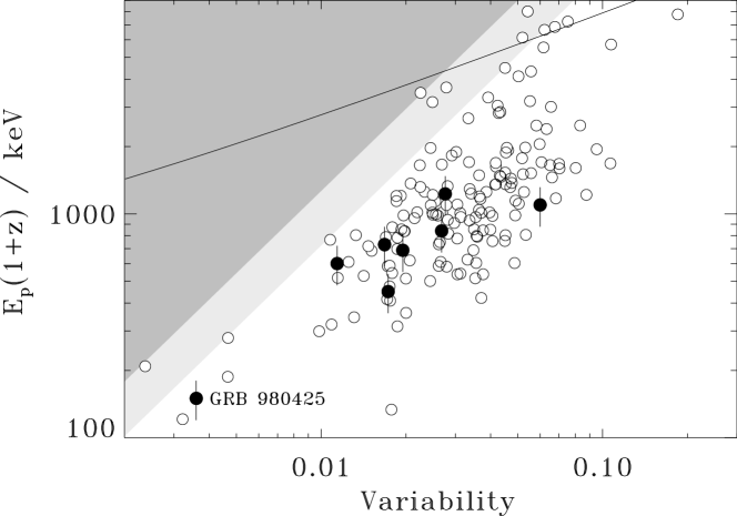
Figure 1.— The peak of the $\nu F_{\nu}$ spectrum in the cosmological rest frame as a function of the burst variability. The filled circles are bursts with secure redshifts estimates, while the empty circles are bursts in which the redshift is derived using the variability-luminosity distance indicator. A trend is clear: the most “spiky” bursts seem to have photons with higher characteristic energies. The shaded regions and solid line indicate where selection effects may play a role, although these effects do not diminish the significance of the correlation. See §3 for details.

Figure 2.— Histogram of intrinsic peak energy $E_{p^{\prime}}=E_{p}(1+z)$ (solid line) for this limited sample. Superposed on the plot (dotted line) is the histogram of the observed peak energy, $E_{p}$.

Figure 3.— Cosmological rest frame peak energy vs. variability (as in Figure 1), but dividing the data into flux bins. The squares, triangles, pentagons, hexagons, and horizontal lines are for $f_{p}=1.5-2.2$ ph/cm²/s, $f_{p}=2.2-2.7$ ph/cm²/s, $f_{p}=2.7-4.0$ ph/cm²/s, $f_{p}=4.0-7.0$ ph/cm²/s, and $f_{p}>7.0$ ph/cm²/s, respectively.

TABLE 1

Trigger	$E_{p}^{(1)}$ (keV)	$f_{p}$ (ph/cm2/s)	V(2)	z(2)
109	450.30	3.62	0.02331	1.79
130	337.10	3.47	0.01681	1.14
143	617.70	47.57	0.05975	2.32
219	263.40	18.06	0.01716	0.58
249	550.90	34.62	0.01698	0.43
394	287.90	4.78	0.01724	1.03
398	180.40	1.71	0.01751	1.63
467	339.30	7.73	0.03122	1.97
503	644.10	5.05	0.07525	10.23
563	280.10	1.89	0.01146	0.85
660	323.00	4.55	0.03047	2.41
676	390.70	4.20	0.02543	1.91
678	1479.00	6.18	0.02256	1.35
761	313.30	3.21	0.03642	3.75
869	523.60	3.52	0.05568	7.27
907	254.90	3.57	0.03864	3.92
973	361.00	5.29	0.04619	4.33
1141	332.50	9.01	0.01417	0.59
1157	223.00	10.04	0.06974	6.26
1288	375.40	6.55	0.02690	1.70
1385	512.70	3.62	0.01919	1.35
1396	219.40	1.68	0.04179	6.41
1440	268.20	11.50	0.05258	3.67
1447	296.30	1.74	0.01511	1.31
1467	166.60	2.26	0.01759	1.46
1468	804.90	3.34	0.05192	6.62
1533	152.30	4.00	0.04895	5.47
1541	337.20	35.58	0.02659	0.81
1578	195.20	3.75	0.01309	0.77
1601	802.80	2.14	0.05419	9.00
1606	253.40	7.82	0.02000	1.03
1623	489.00	2.98	0.02913	2.73
1652	177.80	4.08	0.02440	1.82
1663	617.40	19.00	0.02493	0.97
1712	278.40	3.10	0.03411	3.43
1733	618.20	3.00	0.03920	4.36
1734	93.60	1.70	0.08759	12.00
1886	506.10	16.37	0.10720	10.29
1982	253.00	1.68	0.02786	3.33
1989	92.60	2.73	0.05337	7.71
1993	67.10	1.69	0.03708	5.28
2047	122.90	2.12	0.07029	12.00
2061	464.20	2.19	0.01850	1.59

TABLE 1, continued

Trigger	$E_{p}^{(1)}$ (keV)	$f_{p}$ (ph/cm2/s)	V(2)	z(2)
2080	336.70	5.64	0.01864	1.07
2090	287.40	10.15	0.06066	4.92
2122	115.70	1.89	0.01867	1.72
2123	108.10	2.12	0.00322	0.12
2138	176.40	7.00	0.03126	2.07
2156	423.60	16.57	0.02817	1.22
2193	300.10	1.55	0.02194	2.39
2213	357.00	4.59	0.04568	4.53
2228	235.40	8.10	0.02617	1.49
2232	201.00	6.02	0.06506	7.22
2287	246.90	1.91	0.03372	4.23
2316	196.90	3.83	0.00237	0.06
2340	117.20	1.61	0.04904	8.78
2345	149.60	2.49	0.09533	12.00
2346	143.70	2.93	0.05037	6.73
2383	617.60	3.06	0.03334	3.33
2387	198.10	3.86	0.00984	0.51
2428	439.60	2.05	0.06167	11.61
2443	315.00	2.10	0.02453	2.47
2450	288.10	7.57	0.02618	1.54
2451	80.90	2.82	0.04867	6.46
2533	518.70	8.92	0.01329	0.55
2593	81.20	1.56	0.03764	5.62
2606	324.40	2.38	0.01928	1.63
2681	360.50	1.64	0.04274	6.83
2700	227.90	4.06	0.03705	3.44
2703	348.10	2.89	0.02146	1.75
2780	318.20	1.59	0.01790	1.74
2812	329.80	10.52	0.03637	2.16
2831	590.70	43.43	0.02495	0.68
2855	328.00	9.53	0.01752	0.79
2877	126.40	2.92	0.03556	3.78
2889	381.40	5.92	0.01252	0.60
2890	539.30	2.32	0.02242	2.06
2897	57.60	2.94	0.01777	1.32
2913	146.50	5.20	0.04494	4.17
2922	151.60	2.85	0.03993	4.61
2929	559.30	5.91	0.01852	1.04
2958	146.80	3.75	0.04064	4.15
2984	561.10	4.61	0.03019	2.37
2993	1029.00	3.22	0.02486	2.07
2994	956.90	14.42	0.02448	1.06
3001	238.60	4.19	0.03367	2.92

TABLE 1, continued

Trigger	$E_{p}^{(1)}$ (keV)	$f_{p}$ (ph/cm2/s)	V(2)	z(2)
3003	461.70	2.83	0.01077	0.66
3011	361.70	1.68	0.04332	6.89
3015	226.70	1.75	0.04533	7.30
3035	393.30	6.03	0.01980	1.13
3042	395.70	6.74	0.04173	3.27
3055	152.30	1.78	0.00466	0.23
3057	553.60	32.36	0.02556	0.80
3067	462.10	18.67	0.04507	2.31
3075	181.10	2.32	0.03044	3.29
3093	205.00	2.03	0.04314	6.23
3101	112.00	2.22	0.06610	12.00
3115	298.80	11.10	0.05570	4.09
3128	396.10	12.41	0.03651	2.02
3142	441.30	2.03	0.04237	5.90
3178	680.10	14.34	0.02251	0.94
3212	197.30	2.02	0.04158	5.86
3227	472.80	17.03	0.02600	1.08
3237	218.90	2.01	0.05818	10.34
3241	384.10	12.48	0.03682	2.04
3245	331.50	12.79	0.02065	0.87
3283	203.80	2.57	0.06325	10.75
3287	172.10	6.69	0.02003	1.10
3290	186.10	10.70	0.08028	7.62
3301	477.60	2.81	0.02685	2.48
3306	168.50	3.28	0.02793	2.45
3330	475.80	6.75	0.01962	1.07
3345	220.90	6.76	0.03587	2.58
3352	238.80	3.71	0.00467	0.17
3405	510.80	1.53	0.06217	12.00
3407	176.60	1.53	0.04347	7.29
3408	342.90	12.73	0.02830	1.38
3415	161.20	9.16	0.03529	2.20
3436	236.10	3.56	0.02643	2.17
3448	213.30	2.19	0.03134	3.54
3481	366.60	21.94	0.03968	1.77
3488	292.10	8.65	0.05214	4.15
3489	419.80	6.65	0.01471	0.71
3512	280.70	4.84	0.04175	3.83
3523	799.60	21.57	0.02080	0.71
3569	191.00	4.53	0.08323	12.00
3593	948.80	6.61	0.04503	3.73
3618	363.40	2.50	0.03353	3.69
3634	233.30	3.30	0.05176	6.60

TABLE 1, continued

Trigger	$E_{p}^{(1)}$ (keV)	$f_{p}$ (ph/cm2/s)	V(2)	z(2)
3648	294.00	5.70	0.02971	2.10
3662	546.90	3.05	0.05025	6.53
3663	245.30	4.48	0.04524	4.53
3664	102.90	1.98	0.04518	6.81
3765	328.20	25.29	0.03568	1.43
3788	371.20	5.20	0.01868	1.11
3843	220.40	2.33	0.01787	1.47
3853	598.90	3.08	0.18500	12.00
3891	215.80	13.69	0.03050	1.49
3893	200.50	3.70	0.01089	0.60
3900	90.30	1.53	0.06823	12.00
3912	185.90	4.04	0.03759	3.54
3918	284.00	2.00	0.02486	2.57
3929	355.90	3.97	0.01972	1.35
3954	310.60	8.19	0.04722	3.63
4039	1249.00	5.45	0.02785	1.94
4216	114.60	1.51	0.03475	5.01
5389	197.60	4.14	0.04062	3.96
5470	707.00	4.79	0.06769	8.68
5475	328.20	2.42	0.05522	8.72
5476	135.90	2.55	0.03313	3.60
5479	188.70	2.76	0.04757	6.29
5484	246.00	2.68	0.06557	11.23
5486	303.40	9.35	0.03542	2.19
5489	301.40	9.44	0.04699	3.37
5495	128.70	2.12	0.07006	12.00
5518	213.50	2.35	0.05314	8.27
5526	386.70	3.38	0.02814	2.44
5539	129.30	1.88	0.10660	12.00
5541	147.20	1.66	0.03494	4.80

Table 1Burst trigger number, observed peak energy, photon peak flux, variability, and redshift data used in our analysis.

⁽¹⁾ From fits made to 16 channel data, graciously provided by Robert S. Mallozzi (deceased).

⁽²⁾ From Table 2 of Fenimore & Ramirez-Ruiz (2001).

TABLE 2

$L\propto V^{\beta}$	Eliminate outliers?	Significance	Function
$\beta=3.3$	No	$7\sigma$	$E_{po}\propto V^{0.8\pm 0.15}$
$\beta=3.3$	Yes	$5.5\sigma$	$E_{po}\propto V^{0.7\pm 0.15}$
$\beta=2.2$	No	$5\sigma$	$E_{po}\propto V^{0.5\pm 0.15}$
$\beta=2.2$	Yes	$4\sigma$	$E_{po}\propto V^{0.4\pm 0.15}$
$\beta=5.8$	No	$8\sigma$	$E_{po}\propto V^{1.15\pm 0.15}$
$\beta=5.8$	Yes	$5.5\sigma$	$E_{po}\propto V^{1.05\pm 0.15}$

Table 2Significance and functional form of correlation between $E_{p^{\prime}}$ and $V$ given the best fit, upper and lower limit ($\beta=3.3,\ 2.2,\ 5.8$, respectively) for the $L-V$ relation of Fenimore and Ramirez-Ruiz (2001). We have computed the correlation in each case for the two most severe possible truncations (shaded regions of Figure 1) where the most severe of the two elimates outliers (light shaded region in Figure 1).

References

- (1) Band, D. et al. 1993, ApJ, 413, 281
- (2) Beloborodov, A. M., et al. 2000, ApJ, 535, 158
- (3) Bloom J. S., et al. 1999a, Nature, 401, 453
- (4) Efron, B. & Petrosian, V. 1992, ApJ, 399, 345
- (5) Esin, A. A., & Blandford, R. D. 2000, ApJ, 534, L151
- (6) Fenimore, E. E., et al. 1995, ApJ, 448, L101
- (7) Fenimore, E. E., & Ramirez-Ruiz, E. 2001, ApJ, submitted (astro-ph/0004176)
- (8) Fishman, G., et al. 1992, in Gamma-Ray Bursts: Huntsville, 1991, ed. W. S. Paciesas & G. J. Fishman (New York: AIP), 13
- (9) Galama, T. J., et al. 1998, Nature, 395, 670
- (10) Heise, J., et al. 2001, in Gamma-Ray Bursts in the Aferglow Era: Rome, 2000, in press
- (11) Ioka, K., & Nakamura, T. 2001, ApJ, 554, L163
- (12) Jimenez, R., Band, D. & Piran, T. 2001, ApJ, 561, 171
- (13) Kippen, R. M., et al. 2001, in Gamma-Ray Bursts in the Aferglow Era: Rome, 2000, in press (astro-ph/0102277)
- (14) Kobayashi, S., Ryde, F., & MacFadyen, A. I. 2001, ApJ, submitted (astro-ph/0110080)
- (15) Lazzati, D. et al. 2001, A&A, 378, 996
- (16) Link, B., Epstein, R. I., & Priedhorsky, W. C. 1993, ApJ, 408, L81
- (17) Lloyd, N.M., Petrosian, V., & Mallozzi, R.S. 2000, ApJ, 534, 227
- (18) Lloyd-Ronning, N. M., Fryer, C. L., & Ramirez-Ruiz, E. 2002, ApJ, in press (astro-ph/0108200).
- (19) Lynden-Bell, D. 1971, MNRAS, 155, 95
- (20) Norris, J. P., et al. 1996, ApJ, 459, 2393.
- (21) Norris, J. P., Marani, G. F., & Bonnel, J. T. 2000, ApJ, 534, 248
- (22) Plaga, R. 2001, A&A, 370, 351
- (23) Preece R. D., et al. 2000, ApJS, 126, 19
- (24) Ramirez-Ruiz, E., & Fenimore, E. 1999, Presentation at the 1999 Huntsville GRB conference.
- (25) Ramirez-Ruiz, E., & Fenimore, E. 2000, ApJ, 539, 712
- (26) Ramirez-Ruiz, E., Dray, L., Madau, P., & Tout, C. A. 2000, MNRAS, 327, 829
- (27) Ramirez-Ruiz, E., & Lloyd-Ronning, N. M. 2002, New Astronomy, in press (astro-ph 0203447).
- (28) Salmonson, J.D. 2000, ApJ, 544, L115
- (29) Schaefer, B, E., Ming, D., & Band, D. L. 2001, ApJ, submitted (astro-ph/0101461)
- (30) Reichart, D. E. 1999, ApJ, 521, L111
- (31) Reichart, D. E., et al. 2001, ApJ, 552, 57
- (32) Salmonson, J. D. 2000, ApJ, 544, L115
- (33) Stern, B., Poutanen, J., & Svensson, R. 1997, ApJ, 489, L41
- (34)