Measuring the Size of Quasar Broad-Line Clouds Through
Time Delay Light-Curve Anomalies of Gravitational Lenses

Abstract

Intensive monitoring campaigns have recently attempted to measure the time delays between multiple images of gravitational lenses. Some of the resulting light-curves show puzzling low-level, rapid variability which is unique to individual images, superimposed on top of (and concurrent with) longer time-scale intrinsic quasar variations which repeat in all images. We demonstrate that both the amplitude and variability time-scale of the rapid light-curve anomalies, as well as the correlation observed between intrinsic and microlensed variability, are naturally explained by stellar microlensing of a smooth accretion disk which is occulted by optically-thick broad-line clouds. The rapid time-scale is caused by the high velocities of the clouds ($\sim 5\times 10^{3}~{}{\rm km~{}s^{-1}}$), and the low amplitude results from the large number of clouds covering the magnified or demagnified parts of the disk. The observed amplitudes of variations in specific lenses implies that the number of broad-line clouds that cover $\sim 10\%$ of the quasar sky is $\sim 10^{5}$ per $4\pi$ steradian. This is comparable to the expected number of broad line clouds in models where the clouds originate from bloated stars.

1 Introduction

The use of time delays between the images produced by galaxy scale gravitational lenses to measure the Hubble constant was proposed almost four decades ago (Refsdal 1964). With approximately ten time delays now measured for different lenses (e.g. Kundic et al. 1997; Schechter et al. 1997; Burud et al. 2000), this method has recently become practical (see Kochanek 2002 for a recent summary and analysis). As part of the associated observational effort, Burud (2002) has presented light-curves with very well determined time delays for the systems RX J0911+05 and SBS 1520+530. In both systems Burud (2002) finds evidence for short-term variability which is unique to individual images. The variability is observed on time-scales of tens to hundreds of days, with an amplitude of up to a few percent, and appears to be associated with small intrinsic fluctuations. Similar rapid, low amplitude residual variability has previously been observed between the images of Q0957+561 (Schild 1996). If caused by microlensing within the lens galaxy, this short-term variability is puzzling because naively, the observed amplitudes require very small (non-stellar) microlens masses (Schild 1996) of $m\lesssim 10^{-4}M_{\odot}$ (see also Gould & Miralda-Escudé 1997). Having a dominant microlens population in the required mass range is ruled out by the work of Refsdal et al. (2000) and Wambsganss et al. (2000) on quasar microlensing in Q0957+561 and by Wyithe, Webster & Turner (2000a,b) in Q2237+0305, as well as by Galactic microlensing experiments (e.g. Alcock et al. 2001). Another explanation was suggested by Gould & Miralda-Escudé (1997); in their model rapidly moving hot spots (or cold spots) on the disk surface possess a high transverse velocity and lead to short time-scale variability as the spots move across the stellar microlensing caustics. Since only a small fraction of the source area is magnified, the variability amplitude is small. By postulating the existence of spots with appropriate properties, one might avoid the need to invoke a population of planetary mass microlenses.

In this paper we offer a natural explanation for the observed properties of the short-term variability involving quasar phenomena identified through separate lines of inquiry. We start our discussion with a description of the standard quasar (§2) and microlensing (§3) models. In §4, we explain how the rapid, low-amplitude microlensing observed by Burud (2002) is naturally produced without postulating hypothetical components for either the quasar disk or the lens population. Our model includes typical stellar-mass microlenses, and a featureless accretion disk surrounded by a shell of optically thick broad line clouds, which possess the high velocities and small source sizes necessary to explain the rapid, low amplitude variability. In §5.1 and §5.2 we compare this model against alternative explanations. Finally, we summarize our primary conclusions in § 6. Throughout the paper we assume a flat (filled–beam) cosmology having density parameters of $\Omega_{m}=0.3$ in matter, $\Omega_{\Lambda}=0.7$ in a cosmological constant, and a Hubble constant $H_{0}=65{\rm\,km\,sec^{-1}\,Mpc^{-1}}$.

2 Quasar Model

The UV-optical spectra of nearly all quasars show broad emission lines with Doppler widths of $\sim 5000\,{\rm km\,sec^{-1}}$. The emission is believed to originate from dense clouds having a small filling factor of $\sim 10^{-6}$, which are illuminated by a central ionizing continuum source (see, e.g. Netzer 1990 and references therein). Two popular models were proposed for the origin of the broad line emitters: (i) cool clouds confined within a hot medium (Krolik, McKee & Tarter 1981); and (ii) winds from giant stars which are bloated due their exposure to the intense quasar radiation (Alexander & Netzer 1997 and references therein). The equivalent width of the lines indicates that $\sim 10\%$ of the continuum emission of the quasar is absorbed and reprocessed by the clouds. Hence, the fraction of sky covered by clouds when viewed from the central continuum source, is $F_{\rm c}\sim 0.1$.

The number of clouds, which is important for our analysis is the subject of some controversy. An upper limit for the largest number of individual clouds can be obtained from photo-ionization arguments, yielding $N_{\rm cl}\lesssim 10^{7-8}$ (Arav et al. 1998). In addition, a lower limit on the number of clouds $N_{\rm cl}\gtrsim 10^{7-8}$, has been derived based on the smoothness of the emission lines of NGC 4151 (Arav et al. 1998) and 3C273 (Dietrich et al. 1999), under the assumption that the clouds are confined with a thermal internal velocity dispersion of $\sim 10$–$20~{}{\rm km~{}s^{-1}}$. However the estimated number of clouds is expected to go down dramatically if this assumption is relaxed, bringing the required number to be as small as few times $10^{5}$ for a velocity spread of $\sim 100~{}{\rm km~{}s^{-1}}$ per cloud (H. Netzer, private communication), as expected for the cometary tails of bloated stars. Hence, the observed smoothness of the emission lines does not rule out the bloated star model, which predicts the existence of $10^{4-5}$ clouds per quasar. It was also suggested that the low excitation lines on which the above analysis was based, originate from the outer parts of the accretion disk while the high excitation lines are dominated by discrete emitters (see Dietrich et al. 1999 and references therein). We note that the number of disk-transiting clouds on which we focus in this paper could in principle be significantly smaller than the total number of broad line clouds. First, individual clouds on randomly oriented Keplarian orbits filling a spherical volume might have a distribution preferentially in the plane of the disk (Osterbrock 1993 cited in Dietrich et al. 1999). Second, if the cloud velocity distribution is dominated by an inflow or an outflow bulk velocity, then the number of transiting clouds would also be much smaller than the total (because the radial component of the velocity is much larger than the tangential component). The velocity dispersion of the clouds can be inferred from the line widths, assuming a particular geometry. In this paper we adopt the simplest model, assuming that the velocity distribution of the occulting clouds is randomly oriented in a spherical shell and is induced by the gravitational force of the central black hole. The characteristic distance of the shell from the central source ($\sim 10^{4}$ Schwarzschild radii) is then larger by three orders of magnitude than the scale of the continuum emission region (see, e.g. Peterson 1997).

We model the lensed optical source as an accretion disk surrounded by a large number of optically thick, identical spherical clouds. We adopt the radial surface brightness profile for a thermal accretion disk as computed by Agol & Krolik (1999). The broad line clouds are assumed to be located in a spherical shell of radius $R$ and have orbits with random inclinations around a black hole of mass $M_{\rm bh}$. Based on the virial theorem for the cloud distribution, we get

$$R=\frac{r_{\rm sch}}{2f_{\rm g}}\left(\frac{c}{\sigma_{\rm cl}}\right)^{2},$$ (1)

where $\sigma_{\rm cl}$ is the 1-D velocity dispersion of the broad lines in ${\rm km\,sec^{-1}}$, $r_{\rm sch}=2GM_{\rm bh}/c^{2}$ is the Schwarzschild radius of the black hole, $G$ is the gravitational constant, and $c$ the speed of light. The constant $f_{\rm g}$ depends the geometry of the cloud velocity distribution; in our spherical shell (2-D) geometry $f_{\rm g}=2$ (an isothermal sphere would be described by $f_{\rm g}=3$). Given a total number of clouds $N_{\rm cl}$, the covering fraction is $F_{\rm c}=N_{\rm cl}\pi r_{\rm cl}^{2}/4\pi R^{2}$, where $r_{\rm cl}$ is the physical radius of each cloud. Therefore

$$r_{\rm cl}=R\sqrt{\frac{4F_{\rm c}}{N_{\rm cl}}}$$ (2)

Throughout this paper we show numerical examples with typical parameter values of $M_{\rm bh}=5\times 10^{8}M_{\odot}$, $\sigma_{\rm cl}=5\times 10^{3}\,{\rm km\,sec^{-1}}$ and $F_{\rm c}=0.1$, and assume a face-on disk profile observed in the $R$-band. We show results as a function of the number of clouds, $N_{\rm cl}$, which is the free parameter that is least constrained by existing observations of quasars.

3 Microlensing Model

Throughout most of this paper we consider a fiducial lensing scenario, comprising a lens galaxy at a redshift $z_{\rm d}=0.5$ and a source at $z_{\rm s}=1.5$. We assume typical microlensing parameters encountered just inside the Einstein radius of the lens galaxy, which is modeled as a spherical singular isothermal sphere. In particular, we adopt the likely values of $\kappa_{\star}=0.08$ and $\kappa_{\rm c}=0.46$ for the convergence in stars and smoothly distributed mass, respectively, and a value of $\gamma=0.54$ for the shear (see Wyithe & Turner 2002). The average magnification of the corresponding macro-image is 12.5. The magnification maps for the simulations in this paper were computed with the microlens program kindly provided to us by Joachim Wambsganss.

4 Variability due to Obscuration of the Disk by Broad Line Clouds

Monitoring data of the the systems RX J0911+05 and SBS 1520+530 by Burud (2002) shows evidence for short-term variability which is unique to individual images. The variability is observed on time-scales of tens to hundreds of days, with an amplitude of up to a few percent. Furthermore, the microlensing features appear to be associated with small intrinsic fluctuations. In this section we present a microlensing model that accounts for all three of these features.

4.1 Intrinsic and Microlensing Lightcurves

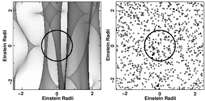
Figure 1: The microlensing geometry. Left: A microlensing magnification map with the contour enclosing 95% of the flux from a face-on thermal accretion disk (Agol & Krolik 1999) around a $5\times 10^{8}M_{\odot}$ black hole. Right: The projection of a shell of $10^{5}$ randomly distributed clouds assuming a covering factor of 10% and a velocity dispersion of 5000 ${\rm km\,s\,^{-1}}$. The lens and source redshifts are $z_{\rm d}=0.5$ and $z_{\rm s}=1.5$. The microlens masses are $m=0.1M_{\odot}$.

Figure 1 shows the geometry of the system. The left panel shows a portion of a magnification map computed for the aforementioned parameter values. Superimposed on this map is a contour enclosing 95% of the flux from the accretion disk source. This contour is displayed again on the right hand panel of Figure 1, together with a random distribution of broad line clouds, whose sizes were computed for $N_{\rm cl}=10^{5}$ [see Eq. (2)]. Since the velocities of the broad line clouds are an order of magnitude larger than the projected transverse velocity expected for the lens galaxy, we assume the accretion disk to be stationary relative to the caustic network. The clouds obscure a fraction $F_{\rm c}=0.1$ of the disk surface. Since the disk surface brightness is a function of radius, the motion of the clouds across regions of varying surface brightness causes low level variability of the total flux. Variability also results from the Poisson noise associated with the variance in the number of obscuring clouds. In the absence of microlensing, and assuming a stationary disk the intrinsic observed flux as a function of time, $t$, is

$$f_{\rm int}(t)=\int_{0}^{\infty}r\,dr\,s_{\nu}(r)-\sum_{i=1}^{N_{\rm cl}}\int_{0}^{r_{\rm cl}}r\,dr\int_{0}^{2\pi}d\theta~{}s_{\nu}\left(\left|\vec{r_{i}}(\frac{t}{1+z_{\rm s}})+\vec{r}\right|\right),$$ (3)

where $s_{\nu}(r)$ is the surface brightness of the disk at frequency $\nu$ and radius $r=|\vec{r}|$, and $\vec{r_{i}}=(r_{i},\theta_{i})$ are the time dependent coordinates of the $N_{\rm cl}$ broad line clouds. If the accretion disk is also subject to microlensing, then the microlensed surface brightness profile is the product of the position-dependent magnification $\mu(\vec{r})$ with the intrinsic accretion disk brightness $s_{\nu}(|\vec{r}|)$. Thus, in the presence of microlensing the light-curve is

$$f_{\rm ml}(t)=\int_{0}^{\infty}r\,dr\int_{0}^{2\pi}d\theta\mu(\vec{r})s_{\nu}(|\vec{r}|)$$

$$-\sum_{i=1}^{N_{\rm cl}}\int_{0}^{r_{\rm cl}}r\,dr\int_{0}^{2\pi}d\theta\mu\left(\vec{r_{i}}(\frac{t}{1+z_{\rm s}})+\vec{r}\right)s_{\nu}\left(\left|\vec{r_{i}}(\frac{t}{1+z_{\rm s}})+\vec{r}\right|\right).$$ (4)

The first term on the right-hand-side of this equation (the magnified flux from the disk) is not a function of time since we have assumed a stationary disk. The variability in the continuum emission due to obscuration by broad line clouds is very different from the variability in the line profiles due to microlensing of the broad line emission itself (Schneider & Wambsganss 1990).

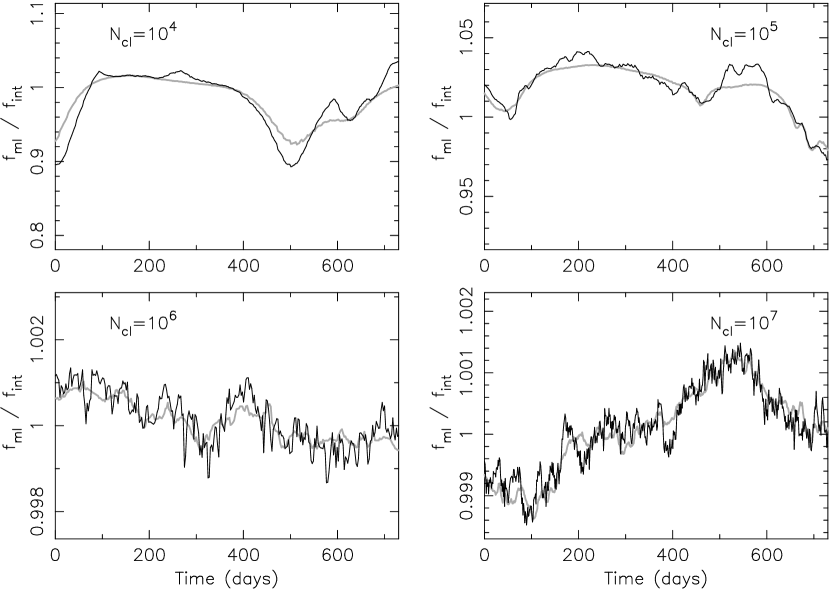
Figure 2: Sample light curves for a disk centered on the position shown in Figure 1. Curves are shown assuming four different cloud sizes corresponding to a total number of clouds per $4\pi$ steradian of $N_{\rm cl}=10^{4}$, $10^{5}$, $10^{6}$ and $10^{7}$. The light line shows the variability in the absence of microlensing, and the dark line shows the variability with microlensing. Note that the vertical axis has a different scale in each case. The lens and source redshifts are $z_{\rm d}=0.5$ and $z_{\rm s}=1.5$.

In Figure 2 we show four sample light-curves corresponding to $N_{\rm cl}=10^{4}$, $10^{5}$, $10^{6}$ and $10^{7}$, all with a duration of two years. The light line shows the level of intrinsic variability $f_{\rm int}(t)$, while the dark line shows variability including microlensing $f_{\rm ml}(t)$. It is apparent that larger clouds produce variability of longer duration and larger amplitude. The amplitudes range from a few percent for the largest clouds under consideration down to hundredths of a percent for the smallest clouds (note that the scaling of the $y$-axis is different in each panel of Figure 2). Similarly, the time-scales for the variability range between tens and hundreds of days. The two curves show similar overall trends, however the peaks and troughs in the microlensed light-curve are more pronounced. The difference between the microlensed and intrinsic variability arise because the variation in effective surface brightness over the accretion disk surface is more extreme in the microlensed case. Keeping in mind the simplicity of our model, the light-curves computed using $N_{\rm cl}\sim 10^{5}$ in Figure 2 show a striking qualitative resemblance to the light-curves presented by Burud (2002), with anomalous microlensing variability superimposed on, and concurrent with, intrinsic light-curve features.

The variability shown in Figure 2 (both $f_{\rm int}$ and $f_{\rm ml}$) is superimposed upon additional longer time-scale intrinsic source variability (common to all of its images), which is observed in unlensed quasars (e.g. Webb & Malkan 2000). We have assumed a population of identical clouds. However for a real quasar we expect a spectrum of cloud sizes with a distribution $\phi(r_{\rm cl})$, representing the number of clouds with radii between $r_{\rm cl}$ and $r_{\rm cl}+\Delta r_{\rm cl}$. Hence, the light-curves reflect a superposition of the corresponding amplitudes and time-scales due to this distribution. The total number of clouds is $N_{\rm cl}^{\rm tot}=\int_{0}^{\infty}dr_{\rm cl}\,\phi(r_{\rm cl})$. However, the effective number of clouds that contribute to the microlensing signal ($N_{\rm eff}$) corresponds to an effective cloud radius $r_{\rm cl}^{\rm eff}$ calculated from the mean of the obscuration area weighted cloud-size distribution. For spherical clouds

$$N_{\rm eff}\sim 4F_{\rm c}\left(\frac{R}{r^{\rm eff}_{\rm cl}}\right)^{2}\hskip 14.22636pt{\rm where}\hskip 14.22636pt(r^{\rm eff}_{\rm cl})^{2}=\frac{\int_{0}^{\infty}dr_{\rm cl}\,r_{\rm cl}^{4}\phi(r_{\rm cl})}{\int_{0}^{\infty}dr_{\rm cl}\,r_{\rm cl}^{2}\phi(r_{\rm cl})}.$$ (5)

The values of $N_{\rm cl}$ quoted in this paper should be identified with $N_{\rm eff}$.

4.2 Variability Statistics

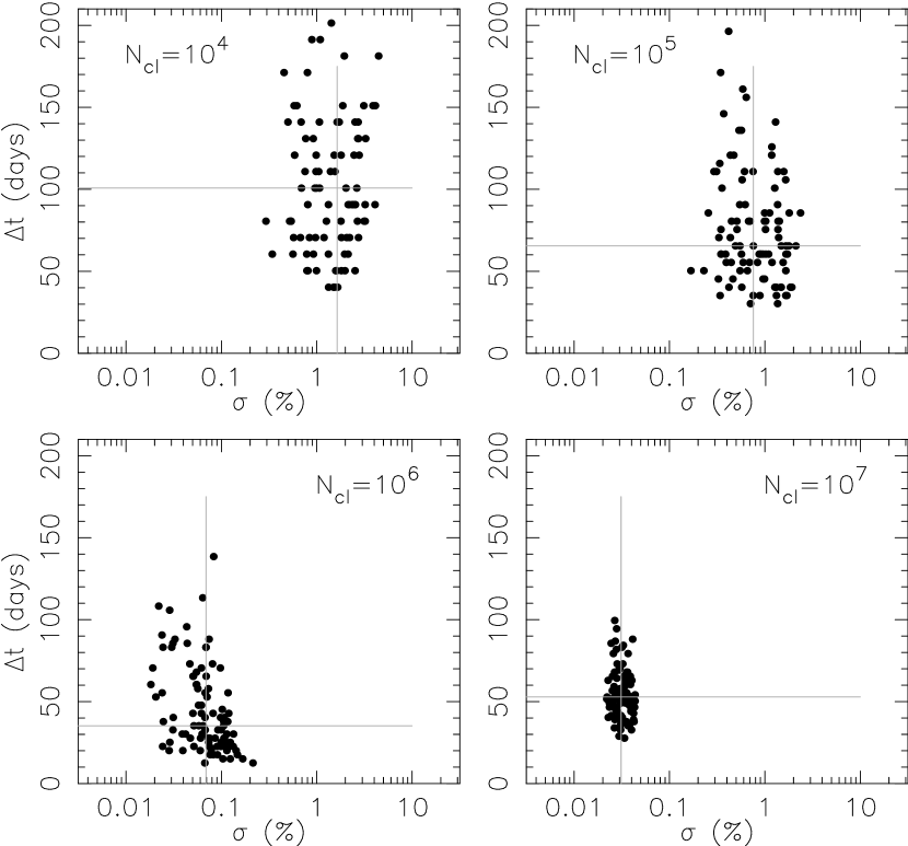
Figure 3: Scatter plots of the correlation time-scale $\Delta t_{\rm corr}$ versus the variance of the variability amplitude $\sigma$ for different source positions on the magnification map. The light lines show the medians of both variables. The four panels correspond to $N_{\rm cl}=10^{4}$, $10^{5}$, $10^{6}$ and $10^{7}$. The lens and source redshifts are fixed at $z_{\rm d}=0.5$ and $z_{\rm s}=1.5$.

The light-curves of Figure 2 demonstrate that bigger clouds produce variability of a longer duration and a larger amplitude. As can be seen from Figure 1, these light-curves were computed (for the purpose of demonstration) using a favorable source location on the magnification map close to several caustics. In this section we present the characteristic time-scales and variability amplitudes for 100 random accretion disk positions across the network of microlensing caustics. Since intrinsic variability will be present in all images of a multiply imaged quasar and only microlensing can produce the anomalous light-curve variability, we calculate variability statistics for the ratio, $f(t)=f_{\rm int}(t)/f_{\rm ml}(t)$ between the intrinsic and microlensed light-curves at each source position. We calculate the autocorrelation function, $f_{\rm AC}(\Delta t)={\rm sign}(f_{\rm AC}^{\prime})\sqrt{|f_{\rm AC}^{\prime}|}$, where $f_{\rm AC}^{\prime}\equiv\langle(f(t)-\langle f\rangle)\times(f(t+\Delta t)-\langle f\rangle)\rangle$. Here, angular brackets denote averaging over long times. The characteristic variability amplitude is taken to be $\sigma=f_{\rm AC}(0)$ (the light-curve variance), and the correlation time-scale $\Delta t_{\rm corr}$ is defined by the condition $f_{\rm AC}(\Delta t_{\rm corr})/f_{\rm AC}(0)=0.5$ for each source position. Figure 3 shows scatter plots of $\Delta t_{\rm corr}$ versus $\sigma$ for $N_{\rm cl}=10^{4}$, $10^{5}$, $10^{6}$ and $10^{7}$. The aforementioned dependence of the time-scale and variability amplitudes on $N_{\rm cl}$ are readily apparent in this plot. The upper panels of Figure 4 show one minus the single variable cumulative probabilities for $\sigma$ and $\Delta t_{\rm corr}$. Characteristic time-scales of 50–100 days are consistent with all cloud sizes, while time-scales below $\sim 50$ days are not consistent with $N_{\rm cl}\lesssim 10^{4}$ and time-scales above $\sim 100$ days are only consistent with $N_{\rm cl}\lesssim 10^{6}$. Inspection of the top-right-hand panel of Figure 4 shows an even stronger dependence on $N_{\rm cl}$. In particular if $N_{\rm cl}\sim 10^{4}-10^{5}$, the variability amplitude is a few tenths of a percent to a few percent, while the variability amplitude is always below $\sigma\sim 0.2\%$ if $N_{\rm cl}\gtrsim 10^{6}$.

Another heavily monitored gravitational lens is Q2237+0305 at an unusually low lens redshift of $z_{\rm d}=0.0394$ (Irwin et al. 1989; Corrigan et al 1991; $\O$stensen et al. 1995; Wozniak et al. 2000a; Wozniak et al. 2000b). The lens was monitored not for the purpose of measuring time delays (for which its geometry is unsuited), but of observing quasar microlensing (for which it is the most favorable lens known). The variability record shows long-term, large amplitude variation, but no variation at the percent level over time-scales of tens of days. Thus if the model proposed in this paper is correct, it must not predict rapid, low amplitude variability in Q2237+0305. To demonstrate the required consistency, we have repeated the calculation described above for a lens galaxy at $z_{\rm d}=0.05$ rather than $z_{\rm d}=0.5$ which closely mimics the Q2237+0305 geometry. The lower panel of Figure 4 shows one minus the single variable cumulative probabilities for $\sigma$ and $\Delta t_{\rm corr}$ as before for $N_{\rm cl}=10^{4}$, $10^{5}$, and $10^{6}$. The median variability for $N_{\rm cl}=10^{4}$ is around $\sigma\sim 1\%$ with a range of $0.1\%\lesssim\sigma\lesssim 5\%$. On the other hand, if $N\gtrsim 10^{5}$ the range is $0.01\%\lesssim\sigma\lesssim 0.5\%$, with a median of $\sigma\sim 0.1\%$. Thus we would not expect a previous detection of short-term anomalous variability in Q2237+0305 if $N_{\rm cl}\gtrsim 10^{5}$. The time-scales are comparable to those for the generic lens case, which is expected since the timescale depends on velocities generated in the source plane rather than the lens plane.

The difference in the statistics of rapid, low amplitude microlensing variability (due to obscuration of the continuum by broad line clouds) between the typical lens geometry ($z_{\rm d}\sim 0.5$) and the special case of a lens at very low redshift ($z_{\rm d}\sim 0.05$) follows from the different size of the projected microlens Einstein radius. The broad-line-cloud induced variability requires that a caustic lie across the accretion disk. In the typical lensing case ($z_{d}=0.5$), the source is relatively large with respect to the caustic network, so that one or more caustics generally cross the source (see Fig. 1). In the low redshift lens case ($z_{d}=0.05$), caustic crossings are rare, and so are the broad line microlensing events. Note that the value of $N_{cl}\sim 10^{5}$ bracketed by the non-detection at $z_{d}=0.05$ and the detection at $z_{d}=0.5$ corresponds to the expected number of broad line clouds in the bloated star model (Alexander & Netzer 1997).

5 Viability of Alternative Explanations

Two alternative explanations for rapid, low amplitude variability appear in the literature. We discuss these in turn, and demonstrate their shortcomings in explaining the observations of RX J0911+05 and SBS 1520+530 by Burud (2002).

5.1 Variability Due to Disk Hot Spots

Gould & Miralda-Escudé (1997) suggested that the observed rapid, low-amplitude variability might result from hot spots on the surface of the disk. This scenario is similar to ours in so far as the short time-scale results from the large orbital velocities in the source plane, while the low amplitude results from the fact that only a small fraction of the total flux is subjected to large amplitude magnification by microlensing. The main differences from our model are that the hot spot velocities ($\sim 0.2c$) are larger than the cloud velocities due to their closer proximity to the black-hole; and the amplitude of fluctuations is governed by the contrast between the surface brightness of the hot spots and the disk, rather than between the opaque clouds and the disk.

We make the simple assumption of circular Keplarian rotation for the hot spots, and distribute a number $N_{\rm sp}$ of them at random within the contour containing 99% of the flux from the disk surface. We assume that the hot spots are long lived for the purpose of the light-curve computation. This is equivalent to the computation of the statistics for the time averaged number of spots. We denote the radius of each spot by $r_{\rm sp}$, and the ratio between the surface brightness of the spot and the disk (locally) by the contrast $C$. Hence, $C=1$ if the spots have the same temperature as the disk, $C=0$ if the spots have zero temperature and contribute no flux (equivalent to the obscuration case presented in the previous section), and $C>1$ for spots that are hotter than the disk. The microlensing light-curve for a stationary disk with hot spots is

$$f_{\rm ml}(t)=\int_{0}^{\infty}r\,dr\int_{0}^{2\pi}d\theta\mu(\vec{r})s_{\nu}(|\vec{r}|)$$

$$+(C-1)\sum_{i=1}^{N_{\rm sp}}\int_{0}^{r_{\rm sp}}r\,dr\int_{0}^{2\pi}d\theta\mu\left(\vec{r_{i}}(\frac{t}{1+z_{\rm s}})+\vec{r}\right)s_{\nu}\left(\left|\vec{r_{i}}(\frac{t}{1+z_{\rm s}})+\vec{r}\right|\right),$$ (6)

where $\vec{r_{i}}=(r_{i},\theta_{i})$ are the time dependent coordinates of the $N_{\rm sp}$ hot spots. This formulation does not result in intrinsic variability.

The parameters for this model are not constrained by observations and we have computed statistics for six representative cases. We assume values for $r_{\rm sp}$ of $10^{14}$cm and $5\times 10^{14}~{}{\rm cm}$, with contrasts of $C=50$ and $C=2$ respectively, resulting in fluctuation amplitudes of $\sim 0.1-1\%$. For each case we compute light-curves for $N_{\rm sp}=1$, 10 and 100. The corresponding fractions of disk covered by the spots are $F_{\rm sp}=0.0001$, 0.001 and 0.01 if $r_{\rm sp}=10^{14}$cm and $F_{\rm sp}=0.0025$, 0.025 and 0.25 if $r_{\rm sp}=5\times 10^{14}$cm. The amplitude of the light-curve scales with $|1+(C-1)F_{\rm sp}|$ and so the results in this section for the amplitude of the fluctuations can be easily generalized to other values of $C$.

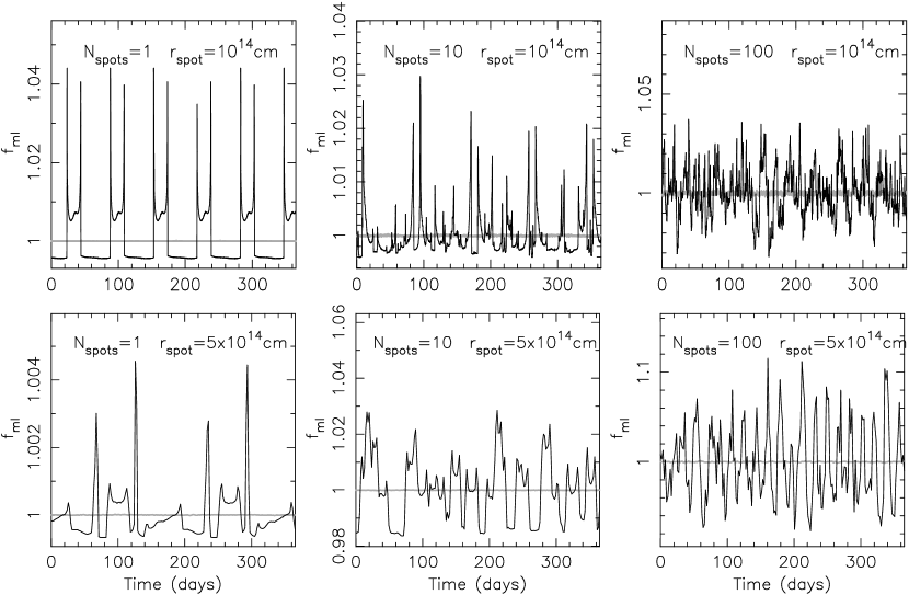
Figure 5: Sample light curves assuming spot radii of $r_{\rm sp}=10^{14}$cm (upper row) and $r_{\rm sp}=5\times 10^{14}$cm (lower row). In each case, light curves resulting from $N_{\rm sp}=1$, 10 and 100 are shown. The light line shows the lack of variability in the absence of microlensing, and the dark line shows the variability due to microlensing. Note that the vertical axis has a different scale in each case. The lens and source redshifts are $z_{\rm d}=0.5$ and $z_{\rm s}=1.5$. The contrast of individual spots in the upper and lower rows is $C=50$ and $C=2$, respectively.

Figure 5 shows sample light-curves for these six cases. The signature of periodicity noted by Gould & Miralda-Escudé (1997) is apparent in the light-curves with a single spot, although for $N_{\rm sp}>1$ the variability is due to the sum of many periodic light-curves with a random phase and the periodicity is diluted. Figure 5 implies that the variability time-scale is shorter than that generated by broad line clouds. Furthermore, if only a few spots are present then the light-curve resembles a classical microlensing light-curve with M-shaped events, but with a reduced amplitude and time-scale. Thus, small numbers of hot spots produce microlensing peaks which look qualitatively different from the troughs produced in the light-curves by the broad line clouds. Moreover, in our formulation, hot spots do not produce intrinsic variability, so that we do not expect microlensing peaks to be concurrent with intrinsic peaks as predicted by the broad line cloud model and observed by Burud (2002).

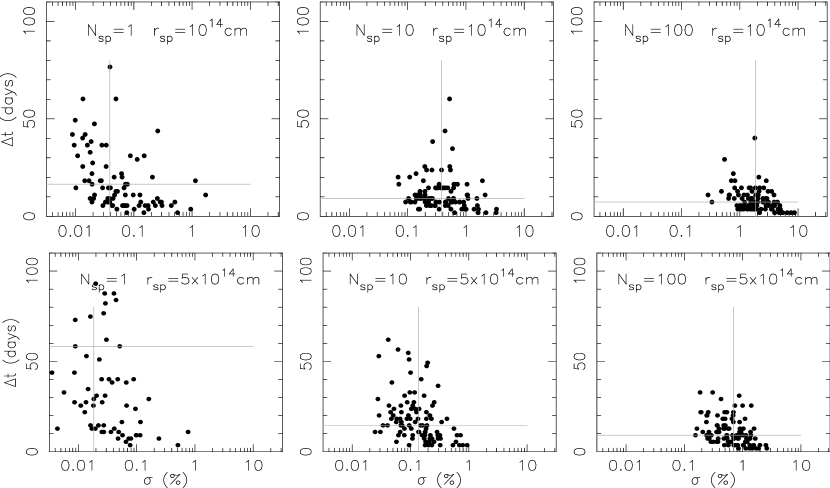
Figure 6: Scatter plots of the correlation time-scale $\Delta t_{\rm corr}$ versus the variance of the variability amplitude $\sigma$ for different source positions. The light lines show the medians of both variables. The upper and lower rows assume spot radii of $r_{\rm sp}=10^{14}$cm and $r_{\rm sp}=5\times 10^{14}$cm. Plots for $N_{\rm sp}=1$, 10 and 100 are shown in each case. The contrast of individual spots in the upper and lower rows is $C=50$ and $C=2$, respectively.

Figure 6 quantifies the variability statistics by showing scatter plots of $\Delta t_{\rm corr}$ versus $\sigma$ for the six cases mentioned above. The variability amplitudes cannot be directly used to constrain $N_{\rm sp}$ or $r_{\rm sp}$ since it is governed by the contrast $C$. However, the time-scales are much shorter than those due to the broad line cloud absorption, with medians below 10–20 days in all cases except for a single large spot ($r_{\rm sp}\sim 15r_{\rm sch}$). Note that this time-scale is nearly independent of the black-hole mass; although a smaller $M_{\rm bh}$ lowers the orbital velocity at a fixed radius, the radius corresponding to a fixed level of disk emission is roughly proportional to $M_{\rm bh}$. Overall, the predicted variability time-scales are shorter than those observed in RX J0911+05 and SBS 1520+530.

5.2 Microlensing by Very Small Masses

We also consider rapid low amplitude microlensing variability due to a population of very low mass compact objects. In this scenario, small amplitude variability results from the source being large compared to the characteristic scale of the caustic network (or equivalently the microlens Einstein radius), while the rapid time-scale results from the short crossing time of this network. We assume a featureless accretion disk without hot spots around a $5\times 10^{8}M_{\odot}$ black hole that moves relative to the caustic network. The transverse velocity $\vec{v}_{\rm gal}$ of the lens galaxy with respect to the observer–source line-of sight is assumed to have a magnitude of $400\,{\rm km\,sec^{-1}}$. The light-curve $f_{\rm ml}(t)$ is

$$f_{\rm ml}(t)=\int_{0}^{\infty}r\,dr\int_{0}^{2\pi}d\theta\mu\left(\vec{r}_{0}+\vec{r}+(t-t_{0})\frac{\vec{v}_{\rm gal}}{1+z_{\rm d}}\frac{D_{\rm s}}{D_{\rm d}}\right)s_{\nu}\left(\left|\vec{r}\right|\right),$$ (7)

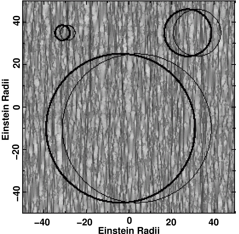
Figure 7: Sample magnification map for very low mass microlenses. The contours enclosing 95% of the flux from a face-on thermal accretion disk (Agol & Krolik 1999) around a $5\times 10^{8}M_{\odot}$ black hole are shown for three microlens masses, namely $m=10^{-2}M_{\odot},10^{-3}M_{\odot}$, and $10^{-4}M_{\odot}$. The pair of circles in each case are shown to demonstrate how far the disk moves during 10 years, assuming a transverse velocity for the lens galaxy of $400\,{\rm km\,sec^{-1}}$. The lens and source redshifts are $z_{\rm d}=0.5$ and $z_{\rm s}=1.5$.

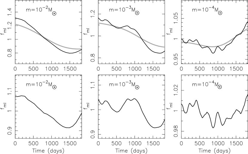
Figure 8: Sample light curves for a smooth accretion disk and very low mass microlenses. Curves are shown for the three microlens masses, $m=10^{-2}M_{\odot},10^{-3}M_{\odot}$ and $10^{-4}M_{\odot}$. In the upper panels the dark lines show raw microlensing light-curves, while the light lines show the light-curves after being Gaussian-smoothed on the correlation time-scale. In the lower panels, the curve shows the ratio between the raw and smoothed curves. The lens and source redshifts are $z_{\rm d}=0.5$ and $z_{\rm s}=1.5$, and the transverse velocity of the lens galaxy is $400\,{\rm km\,sec^{-1}}$.

where $\vec{r}_{0}$ is the quasar position at time $t_{0}$. $D_{d}$ and $D_{s}$ are the angular diameter distances to the lens and source, which we again take to have redshifts $z_{\rm d}=0.5$ and $z_{\rm s}=1.5$. A sample magnification map for very low mass microlenses is shown in Figure 7. Superimposed on this map are the contours enclosing 95% of the flux from a face-on thermal accretion disk assuming three different cases of microlens masses, namely $m=10^{-2}M_{\odot},10^{-3}M_{\odot}$ and $10^{-4}M_{\odot}$. The pair of circles in each case demonstrates how far the disk moves during 10 years. Sample light-curves are shown as the dark lines in the top panel of Figure 8. The light-curves show two characteristic time-scales: a long time-scale governed by the caustic clustering length (see Figure 7) as well as a shorter time-scale.

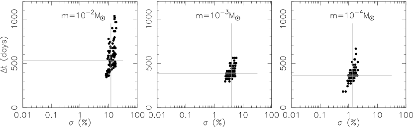
Figure 9: Scatter plots of the correlation time-scale $\Delta t_{\rm corr}$ versus the variance of the variability amplitude $\sigma$ for planetary-mass microlenses. The light lines show the medians of both variables. Plots are shown for microlens masses of $m=10^{-2}M_{\odot},10^{-3}M_{\odot}$ and $10^{-4}M_{\odot}$.

In order to isolate the characteristic amplitude and time-scales of the rapid variability, we performed the following procedure. For each light-curve we find the correlation time as before, and then smooth the light-curve using the correlation time as the standard deviation of a Gaussian smoothing function. The resulting curves are shown by the light lines in the upper panels of Figure 8. The ratio between the two curves yields the rapid, low amplitude variability. These are shown in the lower panels of Figure 8. We constructed autocorrelation functions for a hundred light-curves in each case and extracted the characteristic variability and amplitude as before. The results are shown in Figure 9. We find that the smallest masses under consideration can produce the required variability amplitudes of $\sim 1\%$. However the time-scales are around 400 days, longer than those seen in RX J0911+05 and SBS 1520+530. Note that $\Delta t_{\rm corr}$ is proportional to the inverse of the transverse velocity assumed. The time-scale is also dependent on the direction of the transverse velocity with respect to the microlensing shear. We have conservatively assumed that the direction to be parallel to the shear which results in the most rapid time-scales. However a transverse velocity parallel to the shear can significantly increase $\Delta t_{\rm corr}$ (Wambsganss, Paczynski & Katz 1990; Lewis & Irwin 1996) and make it even less compatible with the data. In addition to the relatively large time-scale for the rapid component of variability, we note that the simulated light-curves differ qualitatively from those observed. The observed light-curves do not show long term microlensing variability over the duration of the monitoring period, as is predicted by this model. Furthermore, since the microlensing variability must be uncorrelated between macro-images, there is no mechanism to explain the correlation between the intrinsic variability and the microlensing variability observed in the light-curves of RX J0911+05 and SBS 1520+530.

To save this model, one might suppose that hot spots are present in addition to the very low mass microlenses. In this way, one might shorten the time-scale predicted by the low mass-microlensing light-curves using the large source plane velocities of the hot-spots, while retaining the low amplitudes for the reasons discussed in § 5.1. However we argue that this scenario will also be inconsistent with the observations. As can be seen from Figure 7, the short ($\sim 400$ day) variability is superimposed on longer term variability that was removed in the above calculations of variability statistics. This long term variability, which is due to the clustering of caustics on scales many Einstein Radii in extent will still be present following the addition of hot spots, but is not seen in the light-curves of RX J0911+05 and SBS 1520+530, which have durations of $\sim 1000-1500$ days. Thus predictions of microlensing variability due to very low mass microlenses differ qualitatively from observations, whether or not the disk has spots.

6 Discussion

We have identified a simple explanation for the anomalous microlensing variability reported by Burud (2002) in the systems RX J0911+05 and SBS 1520+530. We find that the obscuration of a differentially magnified (microlensed) accretion disk by optically-thick broad-line clouds results in rapid variability due to the high cloud velocities and in fluctuations with a low amplitude due to the large number of clouds (and hence small level of Poisson fluctuations). The model predicts fluctuations with an amplitudes (a few percent) and time-scales (50-100 days), comparable to those observed. In addition, the model naturally explains the observed correlation between the intrinsic and microlensing features. The model does not require the inclusion of any hypothetical components.

It is in principle also possible to generate rapid, low amplitude variability through microlensing of hot spots on the surface of an accretion disk (Gould & Miralda-Escudé 1997) or through very low mass microlenses. In the first case, our simulations show that the variability time-scales are substantially shorter than those observed in RX J0911+05 and SBS 1520+530. Of the cases considered, the longer time-scales are produced by a small number of relatively large spots ($r_{\rm sp}\sim 10r_{\rm sch}$). However, a small number of spots produces light-curve shapes that differ qualitatively from those identified in the observations. In the second alternative model of planetary-mass micolenses, we find that the time-scales are governed by the caustic clustering length and source crossing time, rather than the crossing time of the microlens Einstein radius. As a result, the predicted time-scales are longer than those observed.

If our explanation for the nature of this unexpected microlensing signal is correct, it will be of great significance in constraining the properties of the broad line region. Although the dimension of the broad line region is measured by reverberation mapping and the covering factor is known to be $\sim 10\%$, there is currently little information regarding the number and hence the size, of individual broad line clouds (see discussion in §2). Our simple model suggests that to explain the anomalous light-curve features observed by Burud (2002) in RX J0911+05 and SBS 1520+530, the number of broad line clouds that contribute the bulk of the covering factor should be $N_{\rm cl}<10^{6}$. In addition, the lack of these features in Q2237+0305 suggests that $N_{\rm cl}>10^{4}$. Interestingly, these constraints bracket the predicted range for the number of clouds in the bloated star model (Alexander & Netzer 1997).

Our results provide a qualitative explanation for the rapid, low amplitude microlensing variability recently observed in several gravitational lens systems. As more measurements of variability become available in the future for these and other lens system, it will become possible to refine our analysis by detailed modeling of individual systems. The sub-microarcsecond resolution provided by the sensitivity of the rapid microlensing fluctuations to the number of broad line clouds, has the potential to place important constraints on models of the broad line region.

Figure 4: One minus the cumulative probabilities for the correlation time-scale $\Delta t_{\rm corr}$ (left) and the variability variance $\sigma$ (right) for the fiducial time-delay lens case (top, $z_{\rm d}=0.5$ and $z_{\rm s}=1.5$) and for a lensing configuration similar to Q2237+0305 (bottom, $z_{\rm d}=0.05$ and $z_{\rm s}=1.5$). Curves are shown for $N_{\rm cl}=10^{4}$, $10^{5}$, $10^{6}$ and $10^{7}$ (top only).

References

- (1) Agol, E., & Krolik, J. 1999, ApJ, 524, 49
- (2) Alcock, C., et al., 2000, 542, 281
- (3) Alexander, T., Netzer, H., 1997, MNRAS, 284, 967
- Arav et al. (1998) Arav, N., Barlow, T. A., Laor, A., Sargent, W. L. W., & Blandford, R. D. 1998, MNRAS, 297, 990.
- (5) Burud, I., et al., 2000, ApJ., 544, 117
-
(6)
Burud, I., 2002, PhD Thesis, Institut d’Astrophysique,
Liege,
http://vela.astro.ulg.ac.be/themes/dataproc/deconv/theses/burud/ibthese_e.html - (7) Corrigan et al., 1991, Astron. J., 102, 34
- (8) Dietrich, M., Wagner, S.J., Courvoisier, T.J.-L., Bock, H., North, P., 1999, Astron. Astrophys., 351, 31
- (9) Gould, A., Miralda-Escudé, J., 1997, ApJ., 483, L13
- (10) Irwin, M. J., Webster, R. L., Hewitt, P. C., Corrigan, R. T., Jedrzejewski, R. I., 1989, Astron. J., 98, 1989
- (11) Kochanek, C.S., 2002, ApJ., submitted, astro-ph/0204043
- (12) Krolik, J.H., McKee, C.F., Tarter, C.B., 1981, ApJ, 249, 422
- (13) Kundic, T., et al., 1997, ApJ, 482, 75
- (14) Lewis, G.F., Irwin, M.J., 1996, MNRAS, 283, 225
- (15) Netzer, H., 1990, in Blandford, R.D., Netzer, H., Woltjer, L., eds, Saas-Fee Advanced course 20: Active galactic Nuclei. Springer, NewYork, p. 57
- (16) stensen, R. et al. 1996, Astron. Astrophys., 309, 59
- (17) Osterbrock D.E., 1993, ApJ 404, 551
- (18) Peterson, B.M., 1997, An introduction to Active Galactic Nuclei, Cambridge University Press
- (19) Refsdal, S., 1964, MNRAS, 128, 307
- (20) Refsdal, S., Stabell, R., Pelt, J., Schild, R., 2000, Astron. Astrophys., 360, 10
- (21) Schechter, P.L., et al. 1997, ApJ, 475, L85
- (22) Schild, R., 1996, ApJ, 464, 125
- (23) Schneider, P., Wambsganss, J., 1990, Astron. Astrophys, 237, 42
- (24) Webb, W., Malkan, M., 2000, ApJ., 540, 652
- (25) Wozniak, P. R., Alard, C., Udalski, A., Szmanski, M., Kubiak, M, Pietrzynski, G., Zebrun, K., 2000a, Ap. J., 529, 88
- (26) Wozniak, P. R., Alard, C., Udalski, A., Szmanski, M., Kubiak, M, Pietrzynski, G., Zebrun, K., 2000b, Ap. J., 540, L65
- (27) Wambsganss, J., Paczynski, B., Katz, N., 1990, ApJ., 352, 407
- (28) Wambsganss, J., Schmidt, R.W., Colley, W.N., Kundic, T., Turner, E.L., 2000, Astron. Astrophys., 362, L37
- (29) Wyithe, J. S. B, Webster, R. L., Turner, E. L., 2000, MNRAS, 315, 51
- (30) Wyithe, J. S. B, Webster, R. L., Turner, E. L., 2000, MNRAS, 318, 762
- (31) Wyithe, J. S. B, Turner, E. L., 2002, ApJ., accepted, astro-ph/0203214