On leave from ]Canadian Institute for Advanced Research and Department of Physics and Astronomy, University of British Columbia, Vancouver, BC, Canada, V6T 1Z1

Néel order in doped quasi one-dimensional antiferromagnets

Abstract

We study the Néel temperature of quasi one-dimensional S=1/2 antiferromagnets containing non-magnetic impurities. We first consider the temperature dependence of the staggered susceptibility of finite chains with open boundary conditions, which shows an interesting difference for even and odd length chains. We then use a mean field theory treatment to incorporate the three dimensional inter-chain couplings. The resulting Néel temperature shows a pronounced drop as a function of doping by up to a factor of 5.

The study of doped low-dimensional antiferromagnets has been a very active field since the discovery of high-T_c superconductivity. A particularly simple form of doping results from replacing some magnetic Cu ions by non-magnetic ions like Zn. In this case the system is well described by the Heisenberg model with some spins removed from a regular lattice. This problem has been quite extensively studied both theoretically and experimentally in the quasi-two-dimensional case. Recent Monte Carlo simulations have shown convincingly that the zero temperature 2 dimensional system remains Néel ordered for impurity concentrations, $p$ up to the classical percolation threshold, ($p_{c}\approx.407$, on the square lattice) Kato ; Sandvik . An analytic approach has been developed based on spin-wave theory and the T-matrix approximation, valid at impurity concentrations well below percolation, and extended to include weak inter-plane couplings Chernyshev . Recent experiments on La₂Cu_1-x(Zn,Mg)_xO₄ Vajik are consistent with the $T=0$ critical concentration corresponding to classical percolation, and agree in detail, at lower impurity concentrations, with the analytic theory.

Here we study the effect of doping on three dimensional ordering in spin-1/2 chain compounds where the exchange interaction along the chains $J$ is much stronger than the inter-chain coupling $J^{\prime}$. Before doping, the Hamiltonian is

$$H=\sum_{j,\vec{y}}\left(J\vec{S}_{j,\vec{y}}\cdot\vec{S}_{j+1,\vec{y}}+\sum_{\vec{\delta}}J^{\prime}\vec{S}_{j,\vec{y}}\cdot\vec{S}_{j,\vec{y}+\vec{\delta}}\right),$$ (1)

where $J$ is the site-index along the chains and $\vec{\delta}$ are the vectors to neighboring chains. The chain lattice spacing has been set to unity. Randomly removing some of the spins breaks the chains up into finite segments with open boundary conditions, which are still weakly coupled to neighboring chains. This model describes Zn doped Sr₂CuO₃, for example. For the pure system a standard method to study the Néel temperature for weakly coupled chains is to first determine the staggered susceptibility of the one-dimensional chains, $\chi_{1}(T)$. If we then treat the inter-chain couplings in mean field theory MFT we obtain the condition which determines the Néel temperature

$$zJ^{\prime}\chi_{1}(T_{N})=1,$$ (2)

where $z$ is the number of neighboring chains from the sum over $\vec{\delta}$ in Eq. (1). Since at low $T$, $\chi_{1}(T)$ diverges as $1/T$, this predicts $T_{N}\propto J^{\prime}$, so that Néel order is predicted to occur for arbitrarily weak inter-chain coupling.

In this paper we extend this approach to the doped system by calculating the staggered susceptibility of chains with arbitrary length $L$ to find an average value of $\chi_{1}$ as a function of temperature $T$. This type of mean field treatment of inter-plane couplings in doped samples was used to study the Néel temperature of quasi-two-dimensional antiferromagnets in Chernyshev . This method can be carried out much more accurately in the quasi-one-dimensional case studied here because an analytic expression for the staggered susceptibility of finite chains can be found, which by itself yields rather interesting results, exhibiting very different behavior for even and odd length chains. Eq. (2) corresponds to approximating the interchain interactions as simply providing a staggered field of fixed magnitude, acting on a given chain. This approximation results from averaging over both quantum fluctuations and impurity locations on neighboring chains. We expect it to become more reliable when the average chain length $\bar{L}$ and $z$ (i.e. the lattice dimension) increases. Clearly this approximation must break down at large impurity doping $p=1/\bar{L}$, before the percolation threshold is reached ($p_{c}\approx 69.8\%$ for a three dimensional simple cubic lattice). In lower dimensions this approach becomes more questionable since the percolation threshold is reached earlier and the number of neighbors is lower, while in higher dimensions this method may become exact as $z\to\infty$ and valid for all doping levels since $p_{c}\to 1$.

The staggered susceptibility per unit length of a finite chain of length $L$ with open boundary conditions at finite temperature $T=1/\beta$ is

$$\chi_{1}(L,T)\equiv\frac{1}{L}\int_{0}^{\beta}d\tau\sum_{j,k=1}^{L}(-1)^{j-k}\langle S^{z}_{j}(\tau)S^{z}_{k}(0)\rangle.$$ (3)

In order to find a reliable average we need to determine $\chi_{1}$ for a large range of temperatures and lengths for which we use both bosonization techniques and numerical Monte Carlo simulations. Note that here we measure the staggered response to a staggered field, not to be confused with the staggered response to a uniform field impurity .

In order to calculate $\chi_{1}$ as a function of temperature we now go to the continuum limit and use the field theory treatment which is correct in the asymptotic low $T$, large $L$ limit review . The spin operators are then described in terms of a boson field, $\phi$,

$$S^{z}_{j}\approx\frac{\partial_{x}\phi}{\sqrt{2\pi}}+C(-1)^{j}\cos\sqrt{2\pi}\phi,$$ (4)

where $C$ is a parameter which will be discussed in more detail below. The boson field $\phi$ is described by a free massless relativistic Hamiltonian review up to a marginally irrelevant interaction which gives rise to logarithmic corrections as we will see later. We normalize the operator $\cos\sqrt{2\pi}\phi$ so that its $T=0$, $L=\infty$, equal time correlation function decays with distance as $1/2|r|$. In the sum of Eq. (3) we can neglect all rapidly oscillating parts so that only the second term in Eq. (4) will be kept in the alternating spin-spin correlation function

$$G(x,y,\tau)=C^{2}\langle\cos\sqrt{2\pi}\phi(x,i\tau)\cos\sqrt{2\pi}\phi(y,0)\rangle,$$ (5)

so that Eq. (3) becomes

$$\chi_{1}\approx\frac{1}{L}\int_{0}^{\beta}d\tau\int_{0}^{L}dx\int_{0}^{L}dy\,G(x,y,\tau).$$ (6)

To calculate the correlation function we use the mode expansion of the boson for a finite chain with open boundary conditions ourPRB

$$\phi(x,t)=\sqrt{\frac{\pi}{8}}+\sqrt{2\pi}S^{z}\frac{x}{L}+\phi_{>}(x,t),$$ (7)

where

$$\phi_{>}(x,t)\equiv\sum_{n=1}^{\infty}\frac{1}{\sqrt{\pi n}}\sin\frac{\pi nx}{L}\left(e^{-i\pi nvt/L}a_{n}+h.c.\right)$$ (8)

contains the ordinary boson modes $a_{n}$ and the “zero mode” eigenvalue $S^{z}$ corresponds to the z-component of the total spin of the chain, which takes integer values for even lengths $L$ and half-integer values for odd $L$. The spin wave velocity is given by $v=\pi J/2$.

Before considering the case of arbitrary $T$ and $L$, it is interesting to consider the limit $T\to 0$ with $L$ held fixed. In this limit, upon inserting a complete set of states, $\chi_{1}\to{1\over LT}|\langle 0|S^{z}_{\rm alt}|0\rangle|^{2}$ will be dominated by the groundstate $|0\rangle$, where $S^{z}_{\rm alt}\equiv\sum_{j=1}^{L}(-1)^{j+1}S^{z}_{j}$. Using Eq. (7) we can directly find the local staggered magnetization of the lowest energy state in any sector with a given $S^{z}$

$$\langle S^{z}(x)\rangle \approx C(-1)^{x}\langle\cos\sqrt{2\pi}\phi(x)\rangle$$ (9)

$$= C(-1)^{x}\frac{\sin(2\pi S^{z}x/L)}{\sqrt{(2L/\pi)\sin(\pi x/L)}}.$$

For $L$ even $S^{z}=0$ in the groundstate so this gives zero $LT\chi_{1}\to 0$. However, for $L$ odd $S^{z}=\pm 1/2$ in the groundstates, giving

$$\langle\pm|S^{z}(x)|\pm\rangle\approx\pm C(-1)^{x}\sqrt{\frac{\pi}{2L}\sin\frac{\pi x}{L}},$$ (10)

which upon integrating over $x$ gives $S^{z}_{\rm alt}\propto\sqrt{L}$ and therefore $\chi_{1}\propto 1/T$. This divergence is in sharp contrast to the even case. Interestingly Eq. (10) indicates a maximum response in the center of the chain which agrees with numerical results laukamp ; long and is reminiscent of the square-root increase of the staggered response to a uniform field with the distance from the open ends impurity . It is interesting to note that our finding $S^{z}_{\rm alt}\propto\sqrt{L}$ for a spin chain corresponds to an intermediate result between a Néel state with $S^{z}_{\rm alt}=\pm L/2$ and a nearest neighbor dimer state with one unpaired spin $S^{z}_{\rm alt}=\pm 1/2$.

We now consider the case of general $L$ and $T$ using the field theory approach. The correlation function can then be written as

$$G(x,y,\tau)=\frac{C^{2}}{2}\left(\langle e^{i2\pi S^{z}(x-y)/L}\rangle\langle e^{i\sqrt{2\pi}(\phi_{>}(x,i\tau)-\phi_{>}(y,0))}\rangle\right.$$

$$\ \ \ \ \ -\left.\langle e^{i2\pi S^{z}(x+y)/L}\rangle\langle e^{i\sqrt{2\pi}(\phi_{>}(x,i\tau)+\phi_{>}(y,0))}\rangle\right).$$ (11)

Upon using the cumulant theorem for boson modes $\langle e^{A}\rangle=e^{\langle A^{2}\rangle/2}$ we can determine the correlation function at any finite temperature and length by following the analogous calculations in Refs. mattsson and EMK . Using the shorthand notation $u=\pi\frac{x-y-iv\tau}{2L}$, $\bar{u}=\pi\frac{x-y+iv\tau}{2L}$, $w=\pi\frac{x+y+iv\tau}{2L}$, and $\bar{w}=\pi\frac{x+y-iv\tau}{2L}$ we find

$$G(x,y,\tau)=\frac{\pi C^{2}}{4L}\frac{\partial_{x}\theta_{1}(0,e^{-\gamma})}{\sqrt{\theta_{1}(w+u,e^{-\gamma})\,\theta_{1}(w-\bar{u},e^{-\gamma})}}$$

$$\ \ \times\left[B\left(u+\bar{u},e^{-2\gamma}\right)\sqrt{\frac{\theta_{1}(w,e^{-\gamma})\theta_{1}(\bar{w},e^{-\gamma})}{\theta_{1}(u,e^{-\gamma})\theta_{1}(\bar{u},e^{-\gamma})}}\right.$$ (12)

$$\ \ \ -\ \left.B\left(w+\bar{w},e^{-2\gamma}\right)\sqrt{\frac{\theta_{1}(u,e^{-\gamma})\theta_{1}(\bar{u},e^{-\gamma})}{\theta_{1}(w,e^{-\gamma})\theta_{1}(\bar{w},e^{-\gamma})}}\right],$$

where $\theta_{1}$ is the elliptic theta function of the first kind GR . The parameter $\gamma=\frac{v\pi}{2LT}$ gives the spacing in the finite size energy spectrum in relation to the temperature. The contribution $B(x)$ from the zero modes is given by

$$B(z,e^{-2\gamma})\equiv{\sum_{S^{z}}e^{-2\gamma(S^{z})^{2}+2iS^{z}z}\over\sum_{S^{z}}e^{-2\gamma(S^{z})^{2}}}=\frac{\theta(z,e^{-2\gamma)}}{\theta(0,e^{-2\gamma})},$$ (13)

where $\theta$ is the elliptic theta function of the second kind for odd chains $\theta=\theta_{2}$, while it is the elliptic theta function of the third kind for even chains $\theta=\theta_{3}$. Remarkably, the correlation functions in the continuum limit in Eq. (12) therefore retain information about the underlying lattice and explicitly depend on the parity of $L$. This result requires the explicit use of the zero modes in the mode expansion mattsson ; EMK . The difference arises because of the different set of eigenvalues of $S^{z}$: integer and half-integer for even and odd length chains, respectively.

At this point we may rescale all the variables of integration in Eq. (6) by $L$ (or alternatively $T$) to express $\chi_{1}$ in terms of a universal function of the dimensionless variable $LT/v$.

$$\chi_{1}=C^{2}f(LT/v)/T$$ (14)

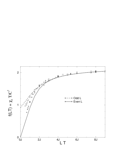
Figure 1: The scaled staggered susceptibility in Eq. (14) $f(LT)=\chi_{1}T/C^{2}$ determined from Eqs. (6) and (12) for even and odd length chains. The upper boundary of the graph represents the asymptotic limit as $LT\to\infty$ in Eq. (15). The points correspond to numerical Monte Carlo results for different combinations of $L$ and $T$ divided by the logarithmic correction in Eq. (18) with $a=23$.

In the thermodynamic limit $LT/v\to\infty$, we can use the asymptotic behavior of the $\theta$ functions GR as was done in a related calculation in mattsson ; EMK for $e^{-\gamma}\to 1$. In this case we can combine the two terms of $G(x,y,\tau)$ in Eq. (12) into one, giving the known finite temperature correlation functions impurity . This results in the well-known $1/T$ behavior benzoate

$$\chi_{1}\ \stackrel{{\scriptstyle\gamma\to 0}}{{\longrightarrow}}\ \frac{C^{2}}{4T}\frac{\Gamma^{2}(1/4)}{\Gamma^{2}(3/4)}\ \approx\ 2.18844\ C^{2}/T$$ (15)

As expected there is no difference between even and odd length chains in the limit of $LT/v\to\infty$ in Eq. (15).

In the opposite limit of zero temperature and finite length $LT/v\to 0$, however, we find a qualitative difference for even and odd chains. Again using asymptotic limits of $\theta$ functions as $e^{-\gamma}\to 0$, we now find

$$G(x,y,\tau)\to\frac{\pi C^{2}}{4L}\sqrt{\frac{\sin(w+u)\sin(w-\bar{u})}{\sin(u)\sin(\bar{u})\sin(w)\sin(\bar{w})}}\times\left\{\begin{array}[]{lcl}1,&\phantom{nn}&\text{L even}\\ &&\\ \cosh(\frac{\pi v\tau}{L}),&\phantom{nn}&\text{L odd}\\ \end{array}\right.$$ (16)

Since for odd $L$ the correlation function $G(x,y,\tau)$ approaches a constant as $\tau\to\infty$ we get a divergence of $\chi_{1}$ in Eq. (6) with $1/T$ for low temperatures, while for even $L$ the integral is proportional to $L$ resulting in

$$\chi_{1}\ \stackrel{{\scriptstyle\gamma\to\infty}}{{\longrightarrow}}\ \left\{\begin{array}[]{lcl}0.92905\ C^{2}L/J,&\phantom{n}&\text{L even}\\ &{}\hfil&\\ \frac{8C^{2}}{\pi T}E^{2}\left(\frac{\pi}{4},\sqrt{2}\right)\approx\ 0.913893\ C^{2}/T,&\phantom{n}&\text{L odd}\end{array}\right.$$ (17)

where $E$ is the elliptic integral of the second kind GR , which can also be derived from Eq. (10). Note that the scaling behavior with $1/T$ in the two limits $LT/v\ll 1$ for odd $L$ in Eq. (17) and $LT/v\gg 1$ in Eq. (15) is the same, up to a factor of about 2. This is of crucial significance for the behavior of the Néel temperature of the doped quasi-one-dimensional system as we shall see.

So far we have ignored the marginally irrelevant interaction mentioned earlier. Its effect on the staggered susceptibility at finite $T$ but $L\to\infty$ is well-known. It corresponds to replacing the constant $C^{2}$ by a slowly varying function of $T$

$$C^{2}=2\sqrt{\ln(aJ/T)/(2\pi)^{3}},$$ (18)

where $a$ is a dimensionless constant exact ; benzoate . From fitting our susceptibility data, we find $a\sim 23$, which gives $C^{2}\approx 0.33\pm 0.07$ for $0.001\lesssim T/J\lesssim 0.2$. A finite length $L$ together with open boundary conditions leads to more complicated logarithmic corrections which may in general involve a different exponent near the boundary Qin . Hence, the general expression of the logarithmic correction at finite $L$ is not known, but we expect that $C^{2}\approx 0.33\pm 0.07$ remains approximately correct for the relevant length scales studied here.

The full behavior of $\chi_{1}$ as a function of the scaling variable $LT$ is shown in Fig. (1) compared to numerical Monte Carlo data after dividing by the logarithmic factor in Eq. (18). There are no adjustable parameters for this fitting except for the constant inside the logarithm $a\approx 23$ and all numerical points from the Monte Carlo simulations fall close to this universal line for larger values of $LT$ as well (not shown). The errors are less than the size of the symbols in the figure so that the deviations are due to higher order corrections. For the simulations we chose different values of $20\lesssim L\lesssim 120$ and $0.025\lesssim T/J\lesssim 0.2$. For $LT\gtrsim 4J$ the even and odd cases are virtually indistinguishable, but as $LT\to 0$ there is a clear difference in the behavior.

Figure 2: The Néel temperature $T_{N}/J^{\prime}$ as a function of $J^{\prime}$ and average chains length $\bar{L}$ from bosonization results (lines) compared to Monte Carlo simulations (symbols).

We now want to determine the Néel temperature by using the mean field treatment of inter-chain couplings in Eq. (2), where $\chi_{1}$ now represents the one-dimensional susceptibility averaged over chain lengths with the probability distribution, $P(L)=e^{-L/\bar{L}}/\bar{L}$, where $\bar{L}$ is the average chain length, corresponding to an impurity concentration of $p=1/\bar{L}$. Because of the scaling form in Eq. (14) it is straightforward to show that the mean field condition in Eq. (2) can be written as

$$T_{N}=C^{2}zJ^{\prime}g(T_{N}\bar{L})$$ (19)

where $g(T_{N}\bar{L})=\int dy\ ye^{-y}f(T_{N}\bar{L}\,y)$ is the average of the scaling function $f$ in Fig. (1) and Eq. (14) and $C^{2}$ is given in Eq. (18) with $T=T_{N}$. We see that the solutions for the Néel temperature $T_{N}/J^{\prime}$ in Eq. (19) are functions of the scaling variable $\bar{L}J^{\prime}$ as shown in Fig. (2) for $z=4$ compared to the results from Monte Carlo simulations. The marginal operator leads to weak logarithmic corrections to this scaling behavior, which leaves the shape of the curve largely unchanged for different $J^{\prime}$, and only shifts it up by a few percent as $J^{\prime}$ is lowered. Therefore we can make a nearly universal quantitative prediction for all doping levels and coupling strengths.

The Néel temperature is strongly affected by doping when the impurity concentration, $1/\bar{L}\geq J^{\prime}/J$ and may drop by as much as a factor of 5, although it remains finite. This is because the scaled average staggered susceptibility $g(T_{N}\bar{L})$ of odd chains is finite as $\bar{L}\to 0$ so that Eq. (19) can always be fulfilled for a positive $T_{N}$. If, however, only even chains were allowed in the system, no non-zero solution would exist for $\bar{L}\lesssim 0.6J/zJ^{\prime}$. As mentioned above, we expect this result to break down at larger impurity doping as the percolation threshold is approached and Néel order disappears.

- (1) K. Kato et al., Phys. Rev. Lett. 84, 4204 (2000).
- (2) A.W. Sandvik, preprint, cond-mat/0110510.
- (3) Y.C. Chen and A.H. Castro-Neto, Phys. Rev. B61, R3772 (2000).
- (4) O.P. Vajik et al., Science, 259, 1691 (2002).
- (5) See, for example I. Affleck, M. Gelfand and R. Singh, J. Phys. A 27, 7313 (1994); I. Affleck and B.I. Halperin, J. Phys. A29, 2627 (1996).
- (6) S. Eggert and I. Affleck, Phys. Rev. Lett. 75, 934 (1995).
- (7) For a review of the conformal field theory treatment of the spin-1/2 chain and earlier references see I. Affleck, Fields, Strings and Critical Phenomena (ed. E. Brézin and J. Zinn-Justin North-Holland, Amsterdam, 1990), p.563.
- (8) S. Eggert and I. Affleck, Phys. Rev. B 46, 10866 (1992).
- (9) A.E. Mattsson, S. Eggert and H. Johannesson, Phys. Rev. B 56, 15615 (1997).
- (10) S. Eggert, A.E. Mattsson and J.M. Kinaret, Phys. Rev. B 56, R15537 (1997).
- (11) I.S. Gradshteyn and I.M. Ryzhik, Table of Integrals, Series, and Products, Academic Press, San Diego, (1994).
- (12) S. Lukyanov, Nucl. Phys. B522, 533 (1998); I. Affleck, J. Phys. A31, 4573 (1998).
- (13) I. Affleck and M. Oshikawa, Phys. Rev. B 60, 1038 (1999).
- (14) V. Brunel, M. Bocquet and T. Jolicoeur, Phys. Rev. Lett. 83, 2821 (1999); I. Affleck and S. Qin, J. Phys. A32, 7815 (1999).
- (15) M. Laukamp, G.B. Martins, C. Gazza, A.L. Malvezzi, E. Dagotto, P.M. Hansen, A.C. Lopez and J. Riera, Phys. Rev. B 57, 10755 (1998).
- (16) S. Eggert and I. Affleck, in preparation.