The Westerbork HI Survey of Spiral and Irregular Galaxies
I. HI Imaging of Late-type Dwarf Galaxies

Neutral hydrogen observations with the Westerbork Synthesis Radio Telescope are presented for a sample of 73 late-type dwarf galaxies. These observations are part of the WHISP project (Westerbork H i Survey of Spiral and Irregular Galaxies). Here we present H i maps, velocity fields, global profiles and radial surface density profiles of H i, as well as H i masses, H i radii and line widths. For the late-type galaxies in our sample, we find that the ratio of H i extent to optical diameter, defined as 6.4 disk scale lengths, is on average $1.8\pm 0.8$, similar to that seen in spiral galaxies. Most of the dwarf galaxies in this sample are rich in H i  with a typical $M_{{H\textsc{i}}}/L_{B}$ of 1.5. The relative H i content $M_{\mathrm{{H\textsc{i}}}}/L_{R}$ increases towards fainter absolute magnitudes and towards fainter surface brightnesses. Dwarf galaxies with lower average H i column densities also have lower average optical surface brightnesses. We find that lopsidedness is as common among dwarf galaxies as it is in spiral galaxies. About half of the dwarf galaxies in our sample have asymmetric global profiles, a third has a lopsided H i distribution, and about half shows signs of kinematic lopsidedness.

1 Introduction

Over the past decades there have been numerous surveys of the H i properties of galaxies using single dish telescopes. These have been useful for determining the global H i properties of galaxies and for finding relations between H i content, morphological type and other global properties. They have been particularly useful for obtaining accurate redshifts and line widths for many galaxies. However, due to the large beam size, imaging galaxies in H i was restricted to the largest galaxies.

With the advent of synthesis radio telescopes H i imaging became routinely possible. Their high spatial resolution inspired many studies of the detailed distribution and kinematics of H i in galaxies. However, most of these studies focused on one or a few galaxies, and only a few studies aimed at obtaining a large sample of field galaxies. Bosma (1978, 1981a,b) and Wevers (1984) both investigated a sample of about 20 galaxies in H i, but these studies focused on large and H i bright galaxies. Broeils & van Woerden (1994) and Rhee & van Albada (1996) investigated larger samples of about 50 galaxies and over a wider range of galaxy properties, but both studies used short observation with the Westerbork Synthesis Radio Telescope (WSRT) so that essentially only one-dimensional data are available. In addition to these studies, there have also been studies of the H i distribution in cluster galaxies. Warmels (1988a) and Cayatte et al. (1990) studied the Virgo Cluster, Verheijen & Sancisi (2001, hereafter VS) the Ursa Major cluster.

To date, little effort has been put into making a large, homogeneous H i imaging survey of the local galaxy population. Clearly, such a survey is important for a systematic study of the H i component, including its kinematical properties and their relation with optical properties. For this reason, the Westerbork H i Survey of Spiral and Irregular Galaxies (WHISP) with the Westerbork Synthesis Radio Telescope (WSRT) was started. The WHISP survey aims at mapping about 500 spiral and irregular galaxies in H i. There are two main aspects to the WHISP project. First, a systematic study of the H i component in itself, covering topics such as the distribution and kinematics of H i in and around galaxies, the frequency of lopsidedness and tidal features in H i, and the variation of these H i properties with the luminous properties and morphological types. Second, the provision of data for other studies, not directly related to the H i component. For example, the kinematic data are of great importance for studies of rotation curves and dark matter properties, the frequency of warps and the understanding of spiral structure. For statistically meaningful results, and for studies of variations with morphological type and luminosity, many hundreds of galaxies need to be observed. The WHISP project will provide the H i maps and velocity fields necessary for this work. These data will be useful for other studies of individual galaxies as well. In addition to the H i data, for all the galaxies in the WHISP sample $R$-band CCD photometry has also been obtained (Swaters & Balcells 2000, hereafter Paper II). These will be used to obtain photometric parameters such as integrated magnitudes, surface brightnesses scale lengths.

This paper focuses on the WHISP H i data for late-type dwarf galaxies. These galaxies in particular have been underrepresented in previous H i synthesis surveys. Nonetheless, as has already been found, these galaxies have interesting properties. Single dish observations have shown that they are generally rich in H i, often with $M_{\mathrm{{H\textsc{i}}}}/L_{B}$ ratios larger than unity (e.g., Roberts & Haynes 1994). The largest H i disks, relative to the optical extent, are found in late-type dwarf galaxies, such as NGC 2915 (Meurer et al. 1996), DDO 154 (Carignan & Purton 1998) and NGC 4449 (Hunter et al. 1998). Rotation curve studies show that these galaxies may have even larger dark matter fractions than ordinary spirals (e.g., Carignan & Beaulieu 1989; Broeils 1992b; Swaters 1999; Côté et al. 2000).

In this paper we present H i observations for a sample of 73 late-type dwarf galaxies and we compare their H i properties with their luminous properties. Sect. 2 describes the sample selection and the observations. Sect. 3 describes the reduction of the data and the derivation of the H i maps and velocity fields, the radial and global profiles, and global properties such as the H i mass, line widths and H i diameters. In section 4 the H i properties of these galaxies are compared to the optical properties, and to the H i and optical properties of bright spiral galaxies. Sect. 5 discusses the occurrence of asymmetries in late-type dwarf galaxies. In Sect. 6 the conclusions are presented.

To facilitate the reading of this paper, all long tables have been put into Appendix A. An atlas of the H i observations is presented in Appendix B.

Figure 1: Histogram of Hubble types in the primary WHISP sample. The shaded area gives the distribution over Hubble types of the sample presented in this paper.

2 The sample

The galaxies for the WHISP survey have so far been selected from the Uppsala General Catalogue of Galaxies (UGC, Nilson 1973), taking observability with the WSRT into account. The typical resolution of the WSRT is $14^{\prime\prime}\times 14^{\prime\prime}/\sin\delta$. To make sure that the galaxies will be sufficiently resolved by the WSRT beam, we first selected galaxies with blue diameters larger than $1.5^{\prime}$ and declinations north of $20^{\circ}$. This resulted in a sample of 3148 galaxies. For 1560 of these H i fluxes are catalogued in the Third Reference Catalogue of Bright Galaxies (hereafter RC3, de Vaucouleurs et al. 1991). Next, the sample was restricted further to galaxies with known H i flux densities larger than 100 mJy, where the H i flux density is the ratio of the integrated H i flux and profile width at the 50% level as listed in the RC3. This resulted in our primary WHISP sample of 409 galaxies. The distribution over morphological types of this sample is shown in Fig. 1. Almost half of the galaxies in the sample selected as described above are late-type dwarf galaxies.

From the primary sample we selected late-type dwarf galaxies, i.e., all galaxies with Hubble types later than Sd, supplemented with galaxies of earlier Hubble type, but with absolute magnitudes fainter than $M_{B}=-17$. Furthermore, we only selected galaxies with H i flux densities larger than 200 mJy and with Galactic latitudes $|b|>10^{\circ}$. This resulted in a sample of 109 galaxies. To this sample we added galaxies that met all selection criteria of the primary WHISP sample, except the diameter criterion. This additional sample consists of 4 galaxies, and these were added to the sample presented in this paper because of the possible uncertainties in using the optical diameter $D_{25}$ as an indicator of the H i diameter (see Sect. 4.1). The combined sample constructed in this way consists of 113 galaxies. The distribution over morphological types of the sample is shown in Fig. 1 as the shaded area. Because the selection is largely based on morphological type, a few galaxies have been included in the sample that have been classified as irregulars, but that proved to be large interacting galaxies rather than dwarf galaxies. Their data are presented here as well.

Out of the sample thus selected, 73 have been observed (these are listed in Table 1). For most of the 40 other galaxies H i data have been obtained by others, although some of these data are as yet unpublished. These 40 galaxies will not be discussed here.

The adopted distances for the galaxies in our sample are listed in Table 1. If available, distances from Cepheids, brightest stars or group membership were used. In case none of these were available, the distance was derived from the systemic velocity, adopting a Hubble constant of $H_{0}=75$ km s^-1 Mpc^-1, and correcting for the Virgocentric inflow following the prescription given in Kraan-Korteweg (1986). A more detailed discussion of the adopted distances and the distance uncertainties is given in Paper II.

3 Observations and reduction

The H i data presented in this paper were obtained with the WSRT between 1992 and 1996. Most galaxies were observed in a single 12 hour synthesis observation. Large galaxies were observed longer to increase the radius of the first grating ring. The typical full resolution is $14^{\prime\prime}\times 14^{\prime\prime}/\sin\delta$. The observations were done with a uniform velocity taper and a channel separation of 2 or 4 km s^-1. The observational setup for each galaxy and the reduction steps are detailed in the WHISP webpages, http://www.astro.rug.nl/$\sim$whisp. Here, we present only a summary of the reduction steps. Unless otherwise stated, the reduction procedure outlined below is the WHISP pipeline reduction as detailed on the WHISP webpages.

The raw UV data were calibrated and flagged interactively, using the NEWSTAR software developed at NFRA at Dwingeloo. Next, the UV data were Fourier transformed to the map plane. Three sets of maps were produced for each galaxy, at the full resolution, at $30^{\prime\prime}\!\times 30^{\prime\prime}$ and at $60^{\prime\prime}\!\times 60^{\prime\prime}$. For each data cube five antenna patterns were calculated, spread evenly through the data cube.

After the maps were constructed, the continuum was subtracted by fitting and subtracting a first order polynomial to the channel maps without H i line emission. Next, the maps were cleaned in the map plane in two steps. First, the areas with H i emission were identified in the $60^{\prime\prime}$ Hanning-smoothed data and masks indicating the areas with emission were constructed by hand. The data were then cleaned, using the masks to define the search areas. Next, the clean components were restored and these data were used to refine the masks. These masks were then used to define the search areas for all three resolutions. Each data cube was cleaned with antenna patterns at the appropriate resolution down to $0.5\sigma$.

3.1 Global profiles, line widths and H i masses

The global profiles were constructed from the flux in the clean components obtained from the $60^{\prime\prime}$ Hanning-smoothed data cubes, after correction for primary beam attenuation. Because the maps were cleaned down to $0.5\sigma$, there is still a small amount of residual flux in the map. In principle, this residual flux may be added to the flux in clean components to give the total flux. There is a pitfall, however. The residual flux is given by the sum over the search area divided by the sum over the antenna pattern. The sum over the antenna pattern varies with the size of the box and may even change sign, possibly resulting in inaccurate values for the residual flux. Therefore, only the flux in the clean components was used to calculate the global profile. On average, the total flux including the residual flux is 2% larger than the flux in the clean components only. Only for 10% of the galaxies, the differences between the two fluxes is larger than 5%, but it is always smaller than 8%. The global profiles for all galaxies are shown in Appendix B.

The H i flux integral for each galaxy has been obtained by adding the fluxes in the clean components, correcting for primary beam attenuation. From this, the H i mass was calculated with the standard formula

$$\mathrm{M}_{\mathrm{{H\textsc{i}}}}=236\cdot\mathrm{D}^{2}\cdot\mathrm{S},$$ (1)

where $\mathrm{M}_{\mathrm{{H\textsc{i}}}}$ is the H i mass in $\mathrm{M}_{\odot}$, D the distance in Mpc and S the H i flux integral in mJy km s^-1. The flux integrals and H i masses are listed in Table 2.

Flux measurements with a synthesis array may underestimate the total flux because of the missing zero and short spacings. The shortest spacings for the present observations were 36 or 72 m, therefore the observations are less sensitive to structures more extended than 5 or 10 arcmin. Because most of the galaxies in our sample are smaller than this limit, the fluxes are in general expected to be well determined. VS found that the WSRT H i fluxes of the galaxies in his sample are in excellent agreement with those obtained from single dish observations (the galaxies in his sample are all smaller than $10^{\prime}$). Comparison of the flux densities derived from the observations presented in this paper to the ones derived from the RC3 data, as used to select our sample, confirms that we are not systematically missing flux. The derived flux densities generally agree, although with a large scatter of about 15%. For galaxies with H i diameters larger than $400^{\prime\prime}$ we seem to miss up to about 10% to 15% of the single dish flux.

From the global profiles the line widths at the 20% and 50% level were derived. For double-horn profiles, the peaks on both sides were used separately to calculate the 20% or 50% levels. In other cases, the overall peaks of the profiles were used. The line-width $W_{20}^{\mathrm{obs}}$ ($W_{50}^{\mathrm{obs}}$) was defined as the difference between the velocities at the 20% (50%) levels on both sides of the global profile. The systemic velocity $v_{\mathrm{sys}}$ was taken to be the average of the midpoints between the profile edges at the 20% and 50% level.

The line widths have been corrected for instrumental broadening using expressions given by VS:

$$\begin{array}[]{l}W_{20}=W_{20}^{\mathrm{obs}}-35.8\left[\sqrt{1+\left(R\over{23.5}\right)^{2}}-1\right]\\ \\ W_{50}=W_{50}^{\mathrm{obs}}-23.5\left[\sqrt{1+\left(R\over{23.5}\right)^{2}}-1\right],\end{array}$$ (2)

where $R$ is the instrumental velocity resolution in km s^-1. Corrections for broadening due to random motions of the H i gas have been calculated with expressions given by Tully & Fouqué (1985):

$$\begin{array}[]{rl}W^{2}_{R,l}\;=\;W^{2}_{l}\kern-7.0pt&+\;W^{2}_{t,l}\;\left[1-2\;e^{-\left(\frac{W_{l}}{W_{c,l}}\right)^{2}}\right]\\ &\\ &-\;2\;W_{l}\;W_{t,l}\left[1-e^{-\left(\frac{W_{l}}{W_{c,l}}\right)^{2}}\right],\end{array}$$ (3)

where the subscript $l$ refers to the line width at the $l=20$% or the $l=50$% level, and $W_{t,l}$ is a term that represents random motions. This formula gives a quadratic subtraction if $W_{l}<W_{c,l}$, and a linear subtraction if $W_{l}>W_{c,l}$ We have adopted $W_{c,20}=120$ km s^-1, $W_{c,50}=100$ km s^-1, $W_{t,20}=32$ km s^-1 and $W_{t,50}=15$ km s^-1 (VS).

3.2 Integrated H i maps

The integrated H i maps were constructed by adding the signal from the cleaned channel maps within the areas defined by the clean masks. Integrated H i maps were constructed at the full resolution, and at $30^{\prime\prime}\!\times 30^{\prime\prime}$ and $60^{\prime\prime}\!\times 60^{\prime\prime}$, using the same masks. These H i maps were corrected for primary beam attenuation.

The H i maps at $30^{\prime\prime}$ resolution are shown in Appendix B. All plots have been displayed on a common gray scale. Note that the noise in an integrated H i map is not constant over the map, because at each position data were added from a different number of channel maps due to the masking used. For uniformly tapered data sets, the noise is given by:

$$\sigma_{tot}=n_{l}^{0.5}\sigma_{c}\sqrt{(n_{c}+n_{l})/(n_{c}-1)},$$ (4)

where $\sigma_{tot}$ is the noise in the integrated H i map and $\sigma_{c}$ the noise in the fit to the line-free channels used to subtract the continuum. The number of channels contributing to the integrated H i maps is given by $n_{l}$, and the number of line-free continuum channels is denoted by $n_{c}$. With this equation a noise map was calculated, which was then used to construct a signal-to-noise map. Using the signal-to-noise map, we selected from the integrated H i map all pixels with a signal-to-noise ratio between 2.75 and 3.25. The average value of these points was then used to define the $3\sigma$ contour indicated by the thick line in the integrated H i maps in the figures in Appendix B.

Figure 2: (a) The intensity weighted mean (IWM) and a Gaussian fit to a skewed model profile. Both the Gaussian fit and the IWM fail to recover the peak velocity, which represents the rotation velocity. The Gaussian fit is closer to the input rotation velocity. (b) The same profile as in panel a, but with a SNR of 3. The Gaussian fit velocity is hardly affected, but the IWM velocity is strongly influenced by the noise. For details see text.

3.3 Velocity fields

The velocity fields were derived in two steps. First, as part of the standard WHISP reduction, a moment analysis was done, which yielded the intensity weighted mean (IWM) velocity field. It is well known that the IWM velocities may suffer from systematic errors. For example, if a profile is skewed (e.g., as a result of beam smearing, high inclination or a thick H i disk), the IWM will yield a value offset from the peak towards the skewed side, as demonstrated in Fig. 2a. A second possible source of systematic error in the IWM velocities is that profiles with low signal-to-noise ratios will be biased to the midpoint of the velocity range of the profile (see Fig. 2b). For a more detailed discussion of the systematic effects that may be introduced if IWM velocities are used, see Swaters (1999).

A better velocity determination is obtained by fitting a single Gauss to the velocity profile, which is less sensitive to asymmetries and noise (see Fig. 2). We therefore determined the velocity fields by fitting a single Gaussian to the line profiles at each position in the Hanning smoothed $30^{\prime\prime}$ resolution data. Initial estimates for the fits were obtained from the moment analysis. Only those fits were used that had amplitudes higher than $3\sigma$. The velocity fields derived in this way are shown in Appendix B.

3.4 Radial H i surface density profiles and H i diameters

The total H i maps have been used to derive radial surface density profiles of H i. Two different methods were used, depending on inclination and angular size. For galaxies with inclinations smaller than about $75^{\circ}$ that are well resolved, the data were azimuthally averaged in concentric ellipses. The orientation parameters used for this are the same as those for the rotation curve analysis (see Swaters 1999). Mostly, these are the same as the optical orientation parameters. The azimuthal averaging was done for the approaching and the receding sides separately. Pixels without measured signal in the total H i map were excluded.

Azimuthal averaging following the above procedure does not produce reliable results for highly inclined galaxies or galaxies that are poorly resolved. For these galaxies the H i radial surface density profiles were derived following the method described by Warmels (1988b). First the total H i maps were integrated parallel to the minor axis, resulting in H i strip integrals. To get the H i surface density profiles, the iterative deconvolution scheme described by Lucy (1974) was applied to the H i strip integrals, with the assumption that the H i distribution is axisymmetric. In short, this method works as follows. An input estimate of the radial profile is converted to a strip integral and smoothed to the resolution of the observations. Next, this strip integral is compared to the observed one, and the input profile is adjusted, and used as input for the next cycle, until a convergence criterion is met. For a detailed description of the procedure, see Warmels (1988b).

In Fig. 3 a comparison is shown between the profiles derived from averaging in ellipses and those based on the Lucy deconvolution scheme. For most galaxies that are not highly inclined, the two profiles agree well, as is seen in Fig. 3 for UGC~5918 and UGC~12732. However, for small and highly inclined galaxies the profiles differ, as expected. For small galaxies, illustrated by UGC~3698 in Fig. 3, the central parts are not resolved, and the Lucy deconvolution restores some of the flux to the central parts. A known problem with this method is that it may restore too much flux to the center. To avoid this, the iteration process to determine the radial profile was stopped after 10 iterations, or at an earlier stage if the derived radial profile matched the observed strip integral at the 95% confidence level, following Warmels (1988b). For edge-on galaxies, averaging over ellipses obviously gives an incorrect result. If the galaxies are optically thin in H i, the Lucy method will give the correct radial H i surface density profile.

Figure 3: Comparison between the radial H i surface density profiles derived from averaging in ellipses (full line) and using the Lucy deconvolution scheme (dotted line).

The surface density profiles have been used to determine the H i radii, $R_{\mathrm{{H\textsc{i}}}}$, defined as the radius where the H i surface density corrected to face-on reaches a density of $1\hbox{\leavevmode\nobreak\ M}_{\odot}/\mathrm{pc}^{-2}$. These radii are given in Table 2.

Most H i surface density profiles are close to exponential in their outer parts. This can be clearly seen in Fig. 4, where the profiles have been plotted on a logarithmic scale and the dotted lines give the exponential fits made to the profile. The derived H i scale lengths are given in Table 2.

Finally, the average H i surface density within 3.2 optical disk scale lengths ($\langle\Sigma_{\mathrm{{H\textsc{i}}}}\rangle_{3.2h}$, where $h$ is the optical disk scale length) was determined, with the optical scale lengths as determined in Paper II. The derived average H i surface densities are listed in Table 2. Use of the optical scale length of the disk has certain advantages over the isophotal radius. The number of optical disk scale lengths within an isophotal radius depends on the central disk surface brightness. The lower the surface brightness, the smaller the number of optical scale lengths within the isophotal radius. For galaxies with very low surface brightnesses, the central surface brightness may even be fainter than the chosen isophotal value and the isophotal diameter would therefore not be defined. The determination of the optical disk scale length, on the other hand, is independent of surface brightness.

To keep our definition of galaxy diameter compatible with the often used isophotal diameters, we defined the galaxy diameter as $6.4h$. This value was chosen because most spiral galaxies for which the isophotal diameter $D_{25}$ has been measured, have an approximately constant central disk surface brightness of 21.65 $B$-mag arcsec^-2 (Freeman 1970), and for these galaxies the 25 mag arcsec^-2 isophote is reached at $3.2h$. Hence, the definition of $6.4h$ as a measure of the galaxy diameter is similar to $D_{25}$ for bright spiral galaxies, but it gives a consistent definition of the galaxy diameter irrespective of surface brightness.

Figure 4: Radial H i surface density profiles (full lines) plotted on a ‘magnitude scale’, i.e., $2.5\log\Sigma_{\mathrm{{H\textsc{i}}}}$, so that the H i scale lengths are defined in the same way as the optical disk scale lengths. The dotted lines represent the exponential fits to the outer parts of the profiles. The UGC numbers are given in the lower left corner of each panel.

Figure 4: continued

The large sample of dwarf galaxies presented here allows a study of the relations between the H i properties of late-type dwarf galaxies and their optical properties. It is important to find out whether the relations found for bright spiral galaxies are also valid for the dwarf galaxy regime. As several studies on the relations between the global properties of late-type dwarf galaxies, based on larger and more complete samples, have already been published (e.g., Roberts & Haynes 1994; Hoffman et al. 1996), we will focus here on H i radii and surface densities. We use the optical data presented in Paper II. Absolute magnitudes, extrapolated central disk surface brightnesses and scale lengths are listed in Table 1.

4 H i properties

4.1 H i diameters versus optical diameters

Figure 5: The H i diameter $D_{\mathrm{{H\textsc{i}}}}$ versus $D_{25}^{\,B,i}$ (a) and $6.4h$ (b). The full line in both panels represents the relation found between $D_{\mathrm{{H\textsc{i}}}}$ and $D_{25}^{\,B,i}$ by Broeils & Rhee (1997).

Broeils & Rhee (1997, hereafter BR) have investigated the H i properties of a sample of spiral galaxies mapped in H i with the WSRT. The sample they use is a combination of the samples of Broeils & van Woerden (1994) and Rhee & van Albada (1996). BR find a strong correlation between the H i diameter $D_{\mathrm{{H\textsc{i}}}}$ (defined at a H i surface density of 1 $\hbox{M}_{\odot}$pc^-2) and the absorption-corrected optical diameter $D_{25}^{\,B,i}$, measured at the 25 $B$-mag arcsec^-2. In Fig. 5a a comparison is shown between the optical and the H i diameters for the late-type dwarf galaxies in our sample. To make this comparison, our $R$-band diameters have been transformed to $B$-band diameters assuming $D_{25}^{\,R,i}/D_{25}^{\,B,i}=1.4$. This ratio was determined from the 46 galaxies for which we have both $R$ and $B$-band data (see Paper II). The full lines in Fig. 5a and b show the relation between $D_{\mathrm{{H\textsc{i}}}}$ and $D_{25}^{\,B,i}$ found by BR (we assumed that for the BR sample $D_{25}^{\,B,i}$ equals $6.4h$). Nearly all galaxies in our sample have much larger H i diameters than expected from the relation found by BR. However, this is most likely due to the choice of the definition of the optical diameter. As argued in Sect. 3, the isophotal diameter $D_{25}^{\,B,i}$ is not a suitable definition if galaxies with different central disk surface brightnesses are compared. For galaxies with lower surface brightnesses, only a smaller fraction of the disk is enclosed within the isophotal diameter. Because most of the dwarfs in this sample have low surface brightnesses, the use of the isophotal diameter $D_{25}^{\,B,i}$ leads to small optical diameters, which could explain the offset seen in Fig. 5a.

Figure 6: Histogram of $D_{\mathrm{{H\textsc{i}}}}/D_{25}^{\,B,i}$ (top panel) and of $D_{\mathrm{{H\textsc{i}}}}/6.4h$ (bottom panel). The horizontal bar in both panels indicates the range of $D_{\mathrm{{H\textsc{i}}}}/D_{25}^{\,B,i}$ for spiral galaxies, as found by Broeils & Rhee (1997).

In Fig. 5b, the relation between optical diameter and H i diameter is shown, but now the optical diameter has been defined as 6.4$h$, as argued above. The scale lengths used in Fig. 5b are $R$-band scale lengths. A comparison of the $B$-band and $R$-band scale lengths for the 46 galaxies for which both bands have been observed showed that on average the scale lengths are similar in both bands (see Paper II). With the optical radius defined as $6.4h$, the late-type dwarf galaxies follow the relation as found by BR. But the relation for dwarf galaxies has a larger scatter than found by BR for brighter spirals, indicating that the optical and H i diameters are less strongly coupled in the dwarf regime, or that the optical and H i diameters are less well defined.

The importance of the definition of optical radius is also seen clearly in Fig. 6, where the distributions of $D_{\mathrm{{H\textsc{i}}}}/D_{25}^{\,B,i}$ and $D_{\mathrm{{H\textsc{i}}}}/6.4h$ are shown. The horizontal bar indicates the average found by BR of $1.7\pm 0.5$. Expressed in units of $D_{25}^{\,B,i}$, the late-type dwarf galaxies have extreme properties, with $D_{\mathrm{{H\textsc{i}}}}/D_{25}^{\,B,i}=3.3\pm 1.5$. In the more suitable units of $6.4h$, the gaseous extent of dwarf galaxies is $D_{\mathrm{{H\textsc{i}}}}/D_{6.4h}=1.8\pm 0.8$. Summarizing, we find that the average H i extent of late-type dwarf galaxies relative to the optical diameter is similar to that of bright spiral galaxies, but with a larger spread. In particular, it seems that the most extended H i disks, relative to the optical disks, are found among dwarf galaxies (e.g., Meurer et al. 1996; Carignan & Purton 1998; Hunter et al. 1998).

Figure 7: H i mass versus H i diameter (filled circles) and versus optical diameter ($6.4h$, open circles). The solid lines represent the fits to the data points. The resulting fit is printed next to the fitted line.

As shown in previous studies (BR; VS), there is a tight relation between H i mass and H i diameter. This relation also holds for dwarf galaxies, as is shown in Fig. 7. The small scatter about this relation points to a small spread in mean H i surface density for the dwarf galaxies in our sample. The H i mass also correlates with the optical diameter, shown in Fig. 7 as well, but with a larger scatter.

Figure 8: The distribution of $M_{\mathrm{{H\textsc{i}}}}/\mathrm{L}_{R}$, the horizontal bars indicate the ranges of $M_{\mathrm{{H\textsc{i}}}}/\mathrm{L}_{R}$ for other morphological types, as found by Broeils & Rhee (1997).

Figure 9: (a) $M_{\mathrm{{H\textsc{i}}}}/\mathrm{L}_{R}$ against absolute $R$-band magnitude, filled circles: late-type dwarfs, open circles: Ursa Major galaxies (Verheijen & Sancisi 1997), crosses: low surface brightness galaxies (de Blok et al. 1996). (b) $M_{\mathrm{{H\textsc{i}}}}/\mathrm{L}_{R}$ versus $R$-band surface brightness. (c) $R$-band surface brightness versus $R$-band magnitude.

4.2 H i mass versus luminosity

Fig. 9 shows the distribution of $M_{\mathrm{{H\textsc{i}}}}/\mathrm{L}_{B}$, where $\mathrm{L}_{B}$ was calculated from $\mathrm{L}_{R}$ assuming a $B-R=0.8$, which is the average $B-R$ colour for the dwarf galaxies in our sample (see Paper II). For comparison, the ranges of $M_{\mathrm{{H\textsc{i}}}}/\mathrm{L}_{B}$ for different morphological types, as derived by BR, are indicated by the horizontal bars. It is clear that the late-type dwarf galaxies have a much higher $M_{\mathrm{{H\textsc{i}}}}/\mathrm{L}_{B}$ than earlier type spiral galaxies, a result already found by Roberts (1969, see also Roberts & Haynes 1994), although for this sample the results may be biased towards higher values because we selected galaxies to have flux densities in excess of 200 mJy. The average value of $M_{\mathrm{{H\textsc{i}}}}/\mathrm{L}_{B}$ for the late-type dwarf galaxies presented here is $1.5\pm 1.0$ $\mathrm{M}_{\odot}/\mathrm{L}_{B,\odot}$.

In Fig. 9 the correlations between $\mu_{0}^{R}$, $M_{R}$ and $M_{\mathrm{{H\textsc{i}}}}/\mathrm{L}_{R}$ are shown. In order to compare the dwarf galaxy properties with those of more luminous spiral galaxies, we have included the results from two other studies. The open circles in Fig. 9 are the Ursa Major galaxies from VS, and the crosses are the low surface brightness galaxies from de Blok, McGaugh & van der Hulst (1996). The full circles are the data from our sample. A clear trend is visible between $\mu_{0}^{R}$ and $M_{\mathrm{{H\textsc{i}}}}/\mathrm{L}_{R}$, in the sense that lower surface brightness galaxies are richer in H i. Also, there appears to be a trend between $M_{R}$ and $M_{\mathrm{{H\textsc{i}}}}/\mathrm{L}_{R}$, although among dwarf galaxies this trend is weak. Fig. 9c shows the weak correlation between $\mu_{0}^{R}$ and $M_{R}$. The dwarf galaxies in our sample have the same range in surface brightness at each absolute magnitude. This is not true of the bright spiral galaxies in the UMa sample of VS, which predominantly have high surface brightnesses. Note that the data presented in Fig. 9 do not represent a complete sample, and some galaxies, such as compact high surface brightness dwarfs or extended low surface brightness galaxies may be missing.

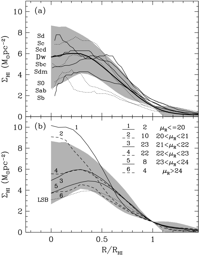
Figure 10: (a) Comparison of the range in radial H i surface density profiles among dwarf galaxies and bright spiral galaxies. The thick black line indicated by ‘Dw’ represents the average profile of all dwarf galaxies in our sample, and the shaded area indicates one standard deviation at each radius around the mean. The other lines represent average profiles for different morphological types from Cayatte et al. (1994). (b) Radial H i surface density profiles of the dwarf galaxies, binned by central disk surface brightness as indicated in the top right. In front of the range in surface brightnesses the number of galaxies in each bin is given. The shaded area is the same as in panel (a). The dotted line is the average profile for LSB galaxies from de Blok et al. (1996).

4.3 H i surface density versus surface brightness

Figure 11: Average H i surface density within 3.2 disk scale lengths ($\langle\Sigma_{\mathrm{{H\textsc{i}}}}\rangle_{3.2h}$) versus central disk surface brightness $\mu_{0}^{R}$.

Inspection of the radial H i surface density profiles in Fig. 4 or in Appendix B, makes it clear that the shapes of the radial H i surface density profiles range from centrally peaked profiles to profiles with central holes. In Fig. 10a the radial density profiles for the galaxies in our sample are compared to the average radial profiles compiled by Cayatte et al. (1994, hereafter CKBG). These authors constructed a comparison sample of radial profiles of undisturbed galaxies based on Warmels (1988c) and Broeils (1992a), as a comparison sample for their Virgo cluster galaxies. CKBG give their profiles in units of $R_{25}$. We converted their profiles to units of $R_{\mathrm{{H\textsc{i}}}}$, using the mean $R_{\mathrm{{H\textsc{i}}}}/R_{25}$ given in CKBG. Because it is confusing to plot all our 73 radial profiles in one figure, the average of all the profiles is shown with the thick line. The shaded area represents one standard deviation at each radius around the mean surface brightness. We note that our selection on flux densities larger than 200 mJy may have introduced a bias towards systems that are rich in H i.

The comparison with the profiles compiled by CKBG shows that the radial profiles found in dwarf galaxies indeed cover a large range shapes, from profiles seen in early-type spirals to those seen in late-type spiral galaxies. Because there is an overlap in morphological types between our sample and late-type spirals, it is not surprising that some of the radial profiles are similar. On the other hand, it is surprising to see that a significant fraction of dwarf galaxies have low H i densities and radial profiles like those found in early-type spiral galaxies. The early type spiral galaxies are believed to have consumed most of their H i and hence have a low H i content. The low H i density dwarf galaxies, on the other hand, are rich in H i, as measured by $M_{\mathrm{{H\textsc{i}}}}/\mathrm{L}_{R}$ (see Fig. 9).

A clue as to why a significant fraction of the dwarf galaxies have low H i densities is provided in Fig. 10b. In this figure, the radial H i density profiles are shown averaged in surface brightness bins. It is clear that galaxies with high optical surface brightnesses have higher H i densities as well. The dwarfs with the lowest surface brightnesses, $\mu_{R}>23$, have radial H i profiles much like those of the LSB galaxies studied by de Blok et al. (1996), shown by the dotted line. These LSB galaxies have central surface brightnesses in the range $22<\mu_{R}<24$. It seems that the H i densities and the luminosity densities are coupled, as was also found by de Blok et al. (1996).

This coupling is explored further in Fig. 11, where the correlation between the average H i density within 3.2 disk scale lengths ($\langle\Sigma_{\mathrm{{H\textsc{i}}}}\rangle_{3.2h}$) and the central surface brightness is shown. The central surface brightness is directly related to the average surface brightness for an exponential disk. Because most of the dwarf galaxies have light profiles close to purely exponential (see Paper II), the central surface brightness has been used in Fig. 11. It is clear that galaxies with higher surface brightnesses have higher H i densities as well. However, the H i density changes much more slowly than the surface brightness in the $R$-band. Over a range of 4 magnitudes in surface brightness, i.e., a factor of 40 in luminosity density, the H i density changes only by about a factor of 4. Therefore, it seems that these galaxies have low H i densities not because they have consumed their H i, like the early type spiral galaxies may have, but because their baryonic mass density in general is lower.

We also investigated whether a correlation exists between H i radial profile shape and absolute magnitude. No such correlation was found; at each absolute magnitude, all profile shapes occur.

5 H i morphology

Large-scale asymmetries in the optical appearance of galaxies have been known for a long time. But galaxies can also be asymmetric in their H i distributions. Baldwin et al. (1980) drew attention to lopsided H i distributions of disk galaxies, emphasizing that the asymmetry affects large parts of the disk and that it is a common phenomenon among spiral galaxies. Richter & Sancisi (1994) made an estimate of the frequency of asymmetries from the shape of the H i line profiles. From an inspection of about 1700 global profiles they found that at least half of the disk galaxies have strong or mild asymmetries. This result was confirmed by Haynes et al. (1998). Swaters et al. (1999) found that lopsidedness may not only be seen in the morphology, but also in the kinematics. They find that probably at least half of all galaxies are kinematically lopsided.

With the present sample of 73 late-type dwarf galaxies, we can investigate the frequency of lopsidedness among dwarf galaxies. To this end, we have inspected the data presented in Appendix B by eye, and looked for lopsidedness in the global profiles, the integrated H i maps and the velocity fields. The results are listed in Table 2.

We find that lopsidedness is as common among dwarf galaxies as it is among spiral galaxies. We find that 25 of the 73 global profiles are clearly asymmetric, and another 12 show mild asymmetries, bringing the total fraction of asymmetric global profiles to about 50%, similar to the fraction seen among spiral galaxies (Richter & Sancisi 1994). The fraction of dwarf galaxies that are lopsided in their H i distribution is about 35%. The fraction of kinematically lopsided dwarf galaxies has been determined from the appearance of the position-velocity diagrams and the velocity fields presented in Appendix B. For 19 galaxies we found that the signal-to-noise ratio was too low to determine whether a lopsidedness in the kinematics was present. For the remaining 54 galaxies, we found that 16 show clear signs of kinematic lopsidedness, and 11 show weak signs, bringing the total at about 50%, concordant with the fraction found in Swaters et al. (1999).

In five of the galaxies the lopsidedness is clearly due to ongoing interaction (UGC~1249, UGC~5272, UGC~5935, UGC~6944 and UGC~7592). In the other cases, there is no clear present interaction. Many of the dwarf galaxies in our sample are members of small groups, and hence are likely to have undergone interaction in the past. The distances to the nearest companions may be large, however, and therefore the excited lopsidedness must be long-lived to explain the high observed fractions of asymmetries in the global profiles, the H i distribution and the kinematics.

5.1 Notes on individual galaxies

UGC~1249 is interacting with the nearby spiral galaxy UGC~1256 which explains its distorted kinematics. The H i to the NE of UGC~1249 is part of a bridge between the two galaxies. We note that these data are somewhat affected by instrumental effects.

UGC~4274 is also known as the Bearpaw Galaxy. The H i in this galaxy is concentrated in one clump that is offset from the optical center. This galaxy was observed in the same pointing as UGC 4278. Because UGC~4274 was far away from the pointing center, the noise at its position was higher after correction for the primary beam attenuation. This explains the large difference between the gray scale and the three sigma contours in the figure in Appendix B.

UGC~4305 shows many holes in its H i distribution. The morphology and kinematics of this galaxy, Holmberg~II, have been studies in detail by Puche et al. (1992).

UGC~5272 has a small companion $2^{\prime}$ to the south, with an H i mass of about $1\cdot 10^{7}$ $\hbox{M}_{\odot}$ and an absolute magnitude of $M_{R}\approx-12.5$. UGC~5272 and its companion are connected by an H i bridge.

UGC~5721 is strongly lopsided in its H i distribution, even though it appears isolated on the sky.

UGC~5935 is interacting with UGC~5931. The extended features in the figure in Appendix B do not represent tidal H i  but are the result of instrumental effects.

UGC~5986 has a strong warp on the SW end. This warp may be related to a small companion, visible in the optical image at the position where the warp sets in. The H i on the NE end appears disrupted as well, with an extension in the same direction as the warp on the SW end. The possible companion does not have H i emission and its redshift is not catalogued, and thus it may be a background galaxy.

UGC~6944 is part of a small group consisting of three bright galaxies. Two of the members contain H i (UGC~6933 and UGC~6944), one has no H i, even though its optically determined systemic velocity falls within the velocity range of these observations. There is some H i seen between the galaxies, most likely as the result of interactions between them.

UGC~7592 has a huge, low column density H i envelope. The H i in the optical part of the galaxy appears to rotate in the opposite sense as the outer H i, although it may also be that the outer H i is warped through the plane of the sky. The properties of the outer H i are studied in more detail in Hunter et al. (1998).

UGC~8490 has a strong warp that is already visible from the morphology of the system, but the kinematics show it more clearly.

6 Conclusions

From the neutral hydrogen observations for the sample of 73 late-type dwarf galaxies presented here, we obtain the following results.

(1) The ratio of the H i extent to the optical diameter, defined as 6.4 disk scale lengths, is on average $1.8\pm 0.8$, similar to the value found for spiral galaxies, but with a larger spread.

(2) Most of the dwarf galaxies in this sample are rich in H i  with typical $M_{\mathrm{{H\textsc{i}}}}/L_{B}$ values of 1.5.

(3) The relative H i content $M_{\mathrm{{H\textsc{i}}}}/L_{B}$ increases towards fainter absolute magnitudes and towards fainter surface brightnesses.

(4) Dwarf galaxies with lower average surface brightnesses also have lower average H i column densities. Over a range of 4 magnitudes in surface brightness, i.e., a factor of 40 in luminosity density, the H i density changes only by about a factor of 4.

(5) We find that lopsidedness is as common among dwarf galaxies as it is in spiral galaxies. About half of the dwarf galaxies in our sample have asymmetric global profiles, a third has a lopsided H i distribution, and about half shows signs of kinematic lopsidedness.

Appendix A Tables

A.1 Table 1 – The sample

Column (1) gives the UGC number. For a description of the sample selection, see Sect. 2.

Column (2) provides other common names, in this order: NGC, DDO (van den Bergh 1959, 1966), IC, Arp (Arp 1966), CGCG. At most two other names are given.

Columns (3) and (4) give the equatorial coordinates (1950) derived from the optical images, as described in Paper II.

Column (5) gives the morphological type according to the RC3, using the same coding.

Column (6) provides the adopted distance. Where possible, stellar distance indicators have been used, mostly Cepheids and brightest stars. If these were not available, a distance based on group membership was used. If this was not available either, the distance was calculated from the H i systemic velocity following the prescription given in Kraan-Korteweg (1986), with an adopted Hubble constant of $H_{0}=75$ km s^-1 Mpc^-1. A full list of published distances for the galaxies in this sample, updated to the beginning of 1998, is given in Table A2 of Paper II. A discussion on the distance uncertainties is given in Sect. 3 of Paper II.

Column (7) gives the absolute $B$-band magnitude, calculated from the apparent photographic magnitude as given in the RC3, and the distance as given in column 6.

Column (8) lists the extrapolated central $R$-band disk surface brightnesses as determined from fits to the surface brightness profiles presented in Paper II. The values have been corrected for Galactic foreground extinction (derived from the $A_{B}$ value according to Burstein & Heiles (1984) assuming $A_{B}/A_{R}$ of 1.77 (Rieke & Lebofsky 1985)), and were corrected to face-on, assuming that the galaxies are transparent.

Column (9) gives the $R$-band disk scale length, as determined from the surface brightness profiles presented in Paper II.

Column (10) gives the diameter at which the 25 $R$-band mag arcsec^-2 is reached, after correction for Galactic foreground extinction and inclination.

A.2 Table 2 – H i properties

Column (1) gives the UGC number.

Column (2) lists the systemic heliocentric velocity.

Column (3) and (4) give the linewidths as determined from the global profile, corrected for random motions and inclinations. Column 3 gives the linewidth at the 20% level, column 4 at the 50% level.

Column (5) contains the integrated H i fluxes derived from the global profiles.

Column (6) lists the H i mass in units of $10^{8}$ $\hbox{M}_{\odot}$.

Column (7) gives the H i radius, defined as the radius where the H i surface density corrected to face-on reaches 1 $\hbox{M}_{\odot}$pc^-2.

Column (8) gives the H i scale length, as determined from a fit to the outer parts of the radial H i density profile.

Column (9) lists the average H i surface density within 3.2 disk scale lengths $\langle\Sigma_{\mathrm{{H\textsc{i}}}}\rangle_{3.2h}$.

Column (10), (11) and (12) indicate whether a galaxy was found to be lopsided in the global profile, the H i distribution or the kinematics. An single star (H) indicates weak lopsidedness, and a double star (HH) strong lopsidedness.

Table 1: The sample

UGC	Other names	R.A. (1950)			Dec. (1950)			Type	Da	$M_{B}$	$\mu_{0}^{R}$	$h$	$D_{25}^{B,i}$
		h m s			∘ ′ ′′				Mpc	mag	mag/${\prime\prime}^{2}$	′′	′′
(1)	(2)	(3)			(4)			(5)	(6)	(7)	(8)	(9)	(10)
731	DDO 9	1	07	46.7	49	20	7	.I..9*.	8.0	-16.6	23.0	46	92
1249	IC 1727	1	44	40.9	27	04	59	.SBS9..	7.5	-17.9	22.1	56	143
1281		1	46	38.9	32	20	31	.S..8..	5.5	-16.2	22.7	46	85
2023	DDO 25	2	30	17.4	33	16	18	.I..9*.	10.1	-17.2	21.8	25	76
2034	DDO 24	2	30	34.4	40	18	34	.I..9..	10.1	-17.5	21.6	26	78
2053	DDO 26	2	31	32.0	29	31	57	.I..9..	11.8	-16.0	22.5	19	43
2455	NGC 1156	2	56	46.5	25	02	21	.IBS9..	7.8	-18.5	19.8	23	111
3137		4	39	21.3	76	19	35	.S?….	18.4	-18.7	24.2	65	48
3371	DDO 39	5	49	49.1	75	18	30	.I..9*.	12.8	-17.7	23.3	53	81
3698		7	05	42.5	44	27	40	.I..9*.	8.5	-15.4	21.2	10	37
3711	NGC 2337	7	06	37.2	44	32	21	.IB.9..	8.6	-17.8	20.9	22	81
3817		7	19	07.9	45	12	18	.I..9*.	8.7	-15.1	22.5	16	36
3851	NGC 2366, DDO 42	7	23	35.1	69	18	53	.IBS9..	3.4	-16.9	22.6	88	207
3966	DDO 46	7	38	01.3	40	13	41	.I..9..	6.0	-14.9	22.2	19	47
4173		7	59	04.6	80	16	10	.I..9*.	16.8	-17.8	24.3	61	35
4274	NGC 2537, Arp 6	8	09	42.8	46	08	28	.SBS9P.	6.6	-18.0	20.7	23	91
4278	IC 2233	8	10	27.5	45	53	43	.SBS7*/	10.5	-17.7	22.5	45	78
4305	Arp 268	8	13	54.9	70	52	46	.I..9..	3.4	-16.8	21.7	60	178
4325	NGC 2552	8	15	40.1	50	09	57	.SAS9$.	10.1	-18.1	21.6	36	105
4499		8	34	01.9	51	49	39	.SX.8..	13.0	-17.8	21.5	22	70
4543		8	39	55.7	45	54	59	.SA.8..	30.3	-19.2	22.0	23	61
5272	DDO 64	9	47	26.8	31	43	16	.I..9..	6.1	-15.1	22.4	21	49
5414	NGC 3104, Arp 264	10	00	56.3	40	59	57	.IXS9..	10.0	-17.6	21.8	30	89
5721	NGC 3274	10	29	30.3	27	55	35	.SX.7?.	6.7	-16.6	20.2	14	62
5829	DDO 84	10	39	54.0	34	42	45	.I..9..	9.0	-17.3	22.4	39	94
5846	DDO 86	10	41	17.2	60	37	52	.I..9..	13.2	-16.1	22.9	19	36
5918	VII Zw 347	10	46	17.6	65	47	41	.I..9*.	7.7	-15.4	24.2	46	27
5935	NGC 3396, Arp 270	10	47	08.3	33	15	20	.IB.9P.	26.4	-20.1	21.8	31	93
5986	NGC 3432, Arp 206	10	49	42.8	36	53	6	.SBS9./	8.7	-18.6	21.4	46	149
6446		11	23	52.9	54	01	20	.SA.7..	12.0	-18.3	21.4	28	95
6628		11	37	25.7	46	13	10	.SA.9..	15.3	-18.8	21.8	36	100
6817	DDO 99	11	48	18.0	39	09	34	.I..9..	4.02	-15.2	23.1	48	84
6944	NGC 3995, Arp 313	11	55	09.8	32	34	19	.SA.9P.	47.4	-21.2	20.4	17	76
6956	DDO 102	11	55	51.4	51	11	48	.SBS9..	15.7	-17.2	23.4	33	51
7047	NGC 4068	12	01	29.6	52	52	7	.IA.9..	3.5	-15.2	21.6	27	81
7125		12	06	10.0	37	04	51	.S..9..	19.5	-18.3	22.8	34	76
7151	NGC 4144	12	07	27.2	46	44	9	.SXS6$/	3.5	-15.7	22.3	44	121
7199	NGC 4163	12	09	37.6	36	26	47	.IA.9..	3.5	-15.1	21.4	22	73
7232	NGC 4190	12	11	13.6	36	54	49	.I..9P.	3.5	-15.3	20.2	15	68
7261	NGC 4204	12	12	42.1	20	56	14	.SBS8..	9.1	-17.7	21.9	35	102
7278	NGC 4214	12	13	08.6	36	36	17	.IXS9..	3.5	-18.3	20.2	53	237
7323	NGC 4242	12	15	01.3	45	53	49	.SXS8..	8.1	-18.9	21.2	54	176
7399	NGC 4288, DDO 119	12	18	10.4	46	34	9	.SBS8..	8.4	-17.1	20.7	18	70
7408	DDO 120	12	18	47.7	46	05	25	.IA.9..	8.4	-16.6	21.9	24	70
7490	DDO 122	12	22	10.4	70	36	39	.SA.9..	8.5	-17.4	21.3	27	90
7524	NGC 4395	12	23	19.9	33	49	26	.SAS9*.	3.5	-18.1	22.2	135	372
7559	DDO 126	12	24	37.5	37	25	9	.IB.9..	3.2	-13.7	23.8	45	49
7577	DDO 125	12	25	15.7	43	46	13	.I..9..	3.5	-15.6	22.5	51	115
7592	NGC 4449	12	25	45.2	44	22	11	.IB.9..	3.5	-18.5	20.3	51	215
7603	NGC 4455	12	26	13.8	23	05	53	.SBS7?/	6.8	-16.9	20.8	21	79
7608	DDO 129	12	26	18.7	43	30	7	.I..9..	8.4	-16.4	22.6	30	68
7690		12	30	01.6	42	58	49	.I..9*.	7.9	-17.0	19.9	12	61

Table 1: – Continued

UGC	Other names	R.A. (1950)			Dec. (1950)			Type	Da	$M_{B}$	$\mu_{0}^{R}$	$h$	$D_{25}^{B,i}$
		h m s			∘ ′ ′′				Mpc	mag	mag/${\prime\prime}^{2}$	′′	′′
(1)	(2)	(3)			(4)			(5)	(6)	(7)	(8)	(9)	(10)
7866	IC 3687	12	39	50.8	38	46	39	.IXS9..	4.8	-15.2	22.1	25	69
7916	I Zw 42	12	41	59.9	34	39	37	.I..9..	8.4	-14.9	24.4	42	26
7971	NGC 4707, DDO 150	12	46	05.9	51	26	16	.S..9*.	8.4	-17.1	21.3	23	77
8188	IC 4182	13	03	30.2	37	52	27	.SAS9..	4.7	-17.4	21.3	52	170
8201	VII Zw 499	13	04	38.2	67	58	21	.I..9..	4.9	-15.8	21.9	32	96
8286	NGC 5023	13	09	58.0	44	18	11	.S..6*/	4.8	-17.2	20.9	34	124
8331	DDO 169	13	13	19.8	47	45	49	.IA.9..	5.9	-15.1	22.9	28	54
8490	NGC 5204	13	27	43.9	58	40	39	.SAS9..	4.9	-17.3	20.5	29	128
8550	NGC 5229	13	31	58.6	48	10	14	.SBS7?/	5.3	-15.6	22.0	24	72
8683	DDO 182	13	40	23.2	39	54	33	.I..9..	12.6	-16.7	22.5	21	42
8837	DDO 185	13	52	56.0	54	08	51	.IBS9./	5.1	-15.7	23.2	50	79
9128	DDO 187	14	13	38.9	23	17	12	.I..9..	4.4	-14.3	21.9	17	50
9211	DDO 189	14	20	38.0	45	36	37	.I..9*.	12.6	-16.2	22.6	19	42
9992		15	41	26.0	67	24	44	.I..9..	10.4	-15.9	22.2	16	39
10310	Arp 2	16	14	49.1	47	10	7	.SBS9..	15.6	-17.9	22.0	25	70
11557		20	23	01.2	60	01	54	.SXS8..	23.8	-19.7	21.0	26	80
11707		21	12	20.3	26	31	36	.SA.8..	15.9	-18.6	23.1	58	94
11861		21	55	44.0	73	01	20	.SX.8..	25.1	-20.8	21.4	53	148
12060		22	28	17.4	33	33	50	.IB.9..	15.7	-17.9	21.6	21	73
12632	DDO 217	23	27	33.0	40	42	55	.S..9*.	6.9	-17.1	23.5	85	120
12732		23	38	09.0	25	57	33	.S..9*.	13.2	-18.0	22.4	35	83

Table 2: HI properties

UGC	$v_{\mathrm{sys}}$	$W_{R,20}^{i}$	$W_{R,50}^{i}$	$\int$Sdv	$M_{\mathrm{HI}}$	$R_{\mathrm{HI}}$	$h_{\mathrm{HI}}$	$\langle\Sigma_{\mathrm{HI}}\rangle_{3.2h}$		lopsidedness
	km s-1	km s-1	km s-1	Jy km s-1	$10^{8}$ $\hbox{M}_{\odot}$	′′	′′	M⊙pc-2		prof.	dens.	kin.
(1)	(2)	(3)	(4)	(5)	(6)	(7)	(8)	(9)		(10)	(11)	(12)
731	639	143	145	48.8	7.4	191	36	5.5		HH		HH
1249	340	129	144	23.5	3.1	362	135	4.3		HH	HH	HH
1281	157	112	113	44.4	3.2	206	60	3.0
2023	603	85	110	18.7	4.5	129	31	4.7
2034	578	103	134	35.8	8.6	189	29	5.5
2053	1029	79	101	17.1	5.6	120	28	6.3		H
2455	380	80	118	71.3	10.2	212	54	10.1
3137	993	218	216	54.5	43.6	297	95	4.0		HH
3371	816	155	159	31.5	12.2	188	31	3.2		HH		H
3698	426	57	63	6.7	1.1	64	39	4.4		HH
3711	433	160	177	39.4	6.9	164	62	7.7
3817	438	72	87	12.9	2.3	103	33	4.5
3851	99	106	111	267.4	7.3	439	118	8.5		HH	HH	HH
3966	361	112	117	24.8	2.1	135	56	6.4		H
4173	862	95	108	31.8	21.2	178	34	3.0		H	HH
4274	447	132	132	14.8	1.5	126	40	5.4		HH	HH
4278	561	161	167	52.3	13.6	193	32	4.1		H		H
4305	158	79	89	246.8	6.7	443	93	7.3
4325	519	185	189	31.2	7.5	142	25	6.6		HH	H	HH
4499	691	138	142	29.8	11.9	143	31	7.2				H
4543	1960	140	157	34.0	73.6	144	71	5.4			H
5272	520	79	102	19.3	1.7	106	22	8.9			HH
5414	612	117	123	27.4	6.5	146	35	6.0		HH	H	HH
5721	537	167	169	62.6	6.6	225	65	11.7		HH	HH
5829	629	119	142	58.2	11.1	188	35	6.7		H
5846	1019	83	95	17.4	7.1	133	31	5.1
5918	338	78	88	21.1	3.0	159	43	2.6			HH
5935	1633	163	178	62.8	103.3	144	104	5.0		HH	HH	HH
5986	616	229	238	151.8	27.1	395	60	6.1		HH	HH	HH
6446	645	152	160	39.7	13.5	182	35	5.5				HH
6628	850	100	110	28.0	15.4	143	35	4.9		H
6817	245	34	53	47.0	1.8	208	131	2.2
6944	3257	189	256	20.3	107.5	123	57	7.1		HH	HH
6956	917	96	122	14.0	8.2	140	38	3.3
7047	211	75	90	38.0	1.1	156	47	8.0		H	HH
7125	1071	135	138	50.0	44.9	240	122	5.3		HH	HH	HH
7151	264	144	144	54.2	1.6	192	19	7.0				HH
7199	164	18	23	9.7	0.3	70	60	3.0
7232	230	55	80	24.5	0.7	112	68	7.8		H
7261	853	153	138	34.3	6.7	159	35	5.2			HH	H
7278	293	121	145	261.7	7.6	447	136	8.3
7323	518	149	157	47.8	7.4	184	35	4.1			HH
7399	535	194	218	44.5	7.4	192	82	7.9		HH	HH	H
7408	462	19	29	9.1	1.5	85	61	2.0			HH
7490	467	161	166	17.5	3.0	142	44	3.3
7524	320	151	154	334.8	9.7	527	50	3.9		HH		HH
7559	218	70	75	30.3	0.7	156	60	3.6		HH	H	HH
7577	196	32	43	28.3	0.8	165	75	2.1			HH
7592	202	191	248	689.2	19.9	698	147	10.0				H
7603	641	126	129	49.1	5.4	192	74	6.3		H	H
7608	537	131	147	33.5	5.6	169	31	5.4		HH		H
7690	537	114	126	24.8	3.7	140	46	8.8			H

Table 2: – Continued

UGC	$v_{\mathrm{sys}}$	$W_{R,20}^{i}$	$W_{R,50}^{i}$	$\int$Sdv	$M_{\mathrm{HI}}$	$R_{\mathrm{HI}}$	$h_{\mathrm{HI}}$	$\langle\Sigma_{\mathrm{HI}}\rangle_{3.2h}$		lopsidedness
	km s-1	km s-1	km s-1	Jy km s-1	$10^{8}$ $\hbox{M}_{\odot}$	′′	′′	M⊙pc-2		prof.	dens.	kin.
(1)	(2)	(3)	(4)	(5)	(6)	(7)	(8)	(9)		(10)	(11)	(12)
7866	359	62	71	23.6	1.3	149	34	4.7
7916	606	64	71	21.6	3.6	140	17	3.1
7971	467	84	99	16.3	2.7	107	27	5.7		H
8188	313	87	116	57.6	3.0	193	38	5.4			HH
8201	37	43	58	35.0	2.0	175	72	3.3		H
8286	407	165	163	65.0	3.5	256	62	4.3				H
8331	260	47	55	17.3	1.4	179	35	1.7		H	HH
8490	204	136	144	140.6	8.0	346	135	9.1		HH
8550	364	113	115	27.7	1.8	172	16	4.0
8683	658	47	49	8.5	3.2	94	26	3.2
8837	144	78	93	26.6	1.6	136	35	1.8		HH		HH
9128	154	43	54	13.9	0.6	87	37	7.5
9211	685	129	132	27.9	10.5	167	42	6.2
9992	427	73	79	11.8	3.0	105	29	5.3		HH		H
10310	713	150	157	21.9	12.6	130	27	6.2				H
11557	1389	155	174	18.9	25.2	142	41	5.0
11707	905	184	186	62.4	37.2	203	37	5.2		HH		HH
11861	1481	296	314	48.0	71.4	194	33	5.1
12060	884	159	171	31.0	18.1	161	58	4.0		HH	HH	H
12632	422	141	145	77.1	8.7	266	43	3.4		HH		HH
12732	749	172	180	89.1	36.6	272	35	4.7		HH		HH

Appendix B Atlas of the H i observations

In the next pages overview figures are presented with the H i data for all the galaxies in the sample. For each galaxy a figure is given with six panels. The H i data shown are at $30^{\prime\prime}$ resolution.

Top left. A grayscale representation of the integrated H i distribution. The contour levels are $1,2,5,8,11,15,20,30,40,50,$ … $10^{20}$ atoms cm^-2. The outermost contour always represents a column density of $1\times 10^{20}$ atoms cm^-2. Contours representing column densities of $5\cdot 10^{21}$ atoms cm^-2 or higher are displayed in white. The thick solid line gives the approximate three sigma level, determined as described in Sect. 3. The plus sign indicates the position of the optical center. The beam size is given in the lower left.

Top right. The velocity field. The thick line is the systemic velocity. The interval between the thin lines is given in the lower left. Light shading indicates receding velocities, dark shading indicates approaching velocities. The extent of the velocity field may be smaller than that of the integrated H i map, because velocities were only determined from profiles with a signal-to-noise ratio higher than three.

Middle left. The integrated H i distribution overlayed on the optical $R$-band image from Paper II.

Middle right. The position-velocity diagram along the major axis. Contour levels are at $-4$ and $-2$ (dotted), and $2\sigma$, $4\sigma$, … .

Bottom left. The radial H i density profile. The thin solid line gives the profile for the approaching side, the dotted line gives the profile for the receding side. The thick solid line is the average radial H i density profile. The vertical arrow indicates a radius of 3.2 optical disk scale lengths.

Bottom right. The global profile. The arrow indicates the systemic velocity.

Full version with figures in this appendix can be downloaded from:

http://www.robswork.net/publications/WHISPI.ps.gz