Dynamic nonlinearity in large scale dynamos with shear

Abstract

We supplement the mean field dynamo growth equation with the total magnetic helicity evolution equation. This provides an explicitly time dependent model for alpha quenching in dynamo theory. For dynamos without shear, this approach accounts for the observed large scale field growth and saturation in numerical simulations. After a significant kinematic phase, the dynamo is resistively quenched, i.e. the saturation time depends on the microscopic resistivity. This is independent of whether or not the turbulent diffusivity is resistively quenched. We find that the approach is also successful for dynamos that include shear and exhibit migratory waves (cycles). In this case however, whether or not the cycle period remains of the order of the dynamical time scale at large magnetic Reynolds numbers does depend how on how the turbulent magnetic diffusivity quenches. Since this is unconstrained by magnetic helicity conservation, the diffusivity is presently an input parameter. Comparison to current numerical experiments suggests a turbulent diffusivity that depends only weakly on the magnetic Reynolds number, but higher resolution simulations are needed.

1 Introduction

The large scale magnetic field of the sun and other stars is frequently modeled using $\alpha\Omega$ dynamo theory (Moffatt 1978; Parker 1979; Krause, & Rädler 1980; Zeldovich, Ruzmaikin, & Sokoloff 1983). This theory has been successful in reproducing the cyclic behavior of solar and stellar activity as well as the latitudinal migration of belts of magnetic activity. The cyclic behavior results mainly from the shear (the $\Omega$ effect); see the references above. Shear also helps producing a strong toroidal field, while the $\alpha$ effect remains responsible for regenerating poloidal from toroidal field. Dynamos without (or weak) shear can also generate large scale fields, but now the $\alpha$ effect also regenerates toroidal from poloidal field ($\alpha^{2}$ dynamo). Such dynamos are usually nonoscillatory. On the other hand, not all $\alpha\Omega$ dynamos are oscillatory: in oblate geometries (accretion discs and galaxies), dynamos tend to be nonoscillatory (e.g., Covas et al. 1999). In simple cartesian geometry with periodic boundaries $\alpha$ effect dynamos always exhibit migratory waves once shear is strong enough.

The viability of an $\alpha$ effect dynamo has been controversial primarily because the nonlinear backreaction of the growing magnetic field on the dynamo coefficients has not been well understood. At the center of the debate is how to incorporate the backreaction into the $\alpha$ effect. It is often taken to be of the form $\alpha=\alpha_{\rm K}\,q(\overline{\bf{B}})$, where $\alpha_{\rm K}$ is the kinematic value and

$$q=\left(1+a\overline{\bf{B}}^{2}/B_{\rm eq}^{2}\right)^{-1}$$ (1)

is a lorentzian quenching function. Here, $\overline{\bf{B}}^{2}$ is the mean field, $B_{\rm eq}$ is the equipartition field strength and $a$ is a dimensionless parameter. In recent years there has been mounting concern that the value of $a$ might actually be of the order of the magnetic Reynolds number, $R_{\rm m}$ (Vainshtein & Cattaneo 1992; Gruzinov & Diamond 1994; 1995; 1996; Bhattacharjee & Yuan 1995; Cattaneo & Hughes 1996), rather than of order unity (e.g., Rüdiger, & Kitchatinov 1993). In stars, $R_{\rm m}\sim 10^{8\ldots 9}$, so quenching would set in for rather weak fields, suggesting that dynamo-generated fields should be much below the equipartition field strength. This is therefore referred to as ‘catastrophic’ quenching.

However, quenchings of the form (1) have traditionally been obtained under the assumption that the system is in a steady state. This leads to incorrect predictions about the evolution of the mean field. Since the magnetic helicity evolution equation must be taken into account, and because it is time dependent, the functional form for $\alpha$ quenching also becomes time dependent. Loosely speaking, a helical field is one with a field-aligned current. While this characterizes primarily the current helicity density, the magnetic helicity is really a volume integral which can be associated with the topological linkage of flux lines. Both magnetic helicity and topological linkage are conserved in the non-resistive (large magnetic Reynolds number) limit. This imposes a crucial constraint on the field evolution in general, and the evolution of the $\alpha$ effect in particular.

There have been a number of important attempts to incorporate dynamical $\alpha$ quenching based on magnetic helicity conservation (Kleeorin & Ruzmaikin 1982; Zeldovich et al. 1983; Kleeorin, Rogachevskii, & Ruzmaikin 1995; see also Seehafer 1996; Ji 1999). Recently Field & Blackman (2002, hereafter FB02) derived from Pouquet, Frisch and Léorat (1976), a simple two-scale approach whose solutions and physical interpretation were shown to agree well with simulations of Brandenburg (2001a, hereafter B01).

Let us define some terms: we refer to the procedure of obtaining $\alpha$ quenching from a time dependent differential equation derived from magnetic helicity conservation as “dynamical” quenching. In this case, $\alpha$ is obtained by solving an explicitly time dependent equation. On the other hand, we refer to the quenching as fixed form or “algebraic” if $\alpha$ is expressed as a fixed function of ${\bf{B}}$, where by fixed we mean that the functional form is kept fixed in time, and the only time dependence enters through ${\bf{B}}$. Although certain algebraic quenching expressions can emerge as a useful approximation in specific temporal regimes, we shall show below that only the dynamical quenching is consistent with the magnetic helicity equation, and the functional form of $\alpha({\bf{B}})$ must change with time. The lorentzian quenching formula (1), when applied for all time, would be an example of a fixed form algebraic quenching prescription.

B01 performed three-dimensional simulations of a zero shear helical dynamo in a periodic domain and found that the field attains super-equipartition field strengths. The initial growth phase is kinematic, and it is only at later times that a saturation phase emerges. The final super-equipartition field strength is reached after a resistive time scale. This behavior can be reproduced empirically by an $\alpha^{2}$ dynamo where both $\alpha$ and turbulent magnetic diffusivity, $\eta_{\rm t}$, are catastrophically quenched according to Eq. (1) with $a\sim R_{\rm m}$ (B01). Below we show however that this form of the turbulent electromotive force is not universal. The dynamical expression is degenerate in special cases where the mean field is current-free or force-free; it therefore reproduces catastrophically quenched behavior in those cases, but not in others.

For an $\alpha^{2}$ dynamo in a periodic box, growth of the large scale magnetic field energy is associated directly with the growth of large scale magnetic helicity. Since the total magnetic helicity can only change resistively, growth of the large scale magnetic helicity implies significant growth of small scale magnetic helicity of the opposite sign. By taking $\alpha$ as proportional to the difference between kinetic and current helicities [the “relative helicity” as derived by Pouquet et al. (1976)] and using a two-scale approach, FB02 developed a model for the nonlinear dynamical quenching of $\alpha$, whose equation for $\alpha$ is formally equivalent to that of Kleeorin & Ruzmaikin (1982) and Zeldovich et al. (1983). Using a two-scale approach, FB02 showed that the growth of the small scale magnetic helicity augments the current helicity contribution to $\alpha$ which ultimately quenches it. The coupling between the small and large scale magnetic helicity equations in this two-scale time dependent dynamical quenching theory predicts that at late times, the quenching of $\alpha$ is consistent with Eq. (1) with $a\sim R_{\rm m}$, but that at early times the dynamo proceeds kinematically, independent of $R_{\rm m}$. The results agree with the simulations of B01 both in terms of the time evolution of the large scale field energy and the saturation value.

An explicitly time dependent quenching formula has sometimes been used in mean-field models, but the main motivation in many instances was to study chaotic behavior in stellar dynamos (Ruzmaikin 1981; Schmalz & Stix 1991; Feudel, Jansen, & Kurths 1993; Covas et al. 1997; 1998). Some kind of dynamical $\alpha$ quenching, but with an explicit time lag, has previously been invoked by Yoshimura (1978) in order to reproduce long term behavior with multiple periods. This approach was however rather ad hoc and not based on magnetic helicity conservation. It was only recently that Kleeorin et al. (1995; 2000) pointed out that the catastrophic quenching of Vainshtein & Cattaneo (1992) can emerge from the dynamical quenching approach under certain circumstances (e.g. when the mean field is current-free or force-free).

The plan of the paper is as follows. In §§2 and 3 we present the governing equations in a form most suitable for our analytic and numerical treatment. We then consider limiting cases such as early and late time evolution, the effective $\alpha$ during the different stages, and the effects of shear (§4). We then consider the full time evolution numerically with and without shear, and compare with fully three-dimensional simulations (§5). Unlike dynamos without shear, dynamos with shear can exhibit dynamo waves and thus cyclic behavior. In addition to being a distinction of astrophysical relevance, we will see that this distinction is important in assessing the role of turbulent diffusion. Finally, we present possible extensions of the model (§6) and present our conclusions (§7).

2 The dynamical equation for $\alpha$

We use the magnetic helicity equation for the fluctuating field as an auxiliary equation that needs to be solved simultaneously with the mean-field dynamo equation. For the $\alpha^{2}$ dynamo case, the dynamical quenching theory derived below is similar to that of FB02, but here we generalize the approach to the $\alpha\Omega$ dynamo.

In a closed or periodic domain the magnetic helicity, $\langle{\bf{A}}\cdot{\bf{B}}\rangle$, evolves according to

$${{\rm d}{}\over{\rm d}{}t}\langle{\bf{A}}\cdot{\bf{B}}\rangle=-2\eta\mu_{0}\langle{\bf{J}}\cdot{\bf{B}}\rangle,$$ (2)

where ${\bf{A}}$ (with ${\bf{B}}=\mbox{\boldmath$\nabla$}{}\times{\bf{A}}$) is the magnetic vector potential, ${\bf{J}}=\mbox{\boldmath$\nabla$}{}\times{\bf{B}}/\mu_{0}$ is the current density, $\eta$ is the microscopic magnetic diffusivity, and angular brackets denote volume averages. We split the magnetic field into mean and fluctuating components, i.e. ${\bf{B}}=\overline{\bf{B}}+{\bf{b}}$ (and similarly for all other quantities). Mean fields are here defined by averaging over one or two coordinate directions, depending on whether the mean field is two- or one-dimensional; see below. The evolution of the mean magnetic vector potential is given by

$${\partial\overline{\bf{A}}\over\partial t}=\overline{\mbox{\boldmath${\cal E}$}}{}+\overline{\bf{U}}\times\overline{\bf{B}}-\eta\mu_{0}\overline{\bf{J}}-\mbox{\boldmath$\nabla$}{}\overline{\phi},$$ (3)

where $\overline{\mbox{\boldmath${\cal E}$}}{}=\overline{{\bf{u}}\times{\bf{b}}}$ is the electromotive force resulting from small scale velocity and magnetic fields, and $\overline{\phi}$ is the electrostatic potential of the mean field which can be chosen arbitrarily without affecting the magnetic field and magnetic helicity. From Eq. (3) one obtains an evolution equation for the magnetic helicity of the mean field,

$${{\rm d}{}\over{\rm d}{}t}\langle\overline{\bf{A}}\cdot\overline{\bf{B}}\rangle=2\langle\overline{\mbox{\boldmath${\cal E}$}}{}\cdot\overline{\bf{B}}\rangle-2\eta\mu_{0}\langle\overline{\bf{J}}\cdot\overline{\bf{B}}\rangle,$$ (4)

and an evolution equation for the magnetic helicity of the fluctuating field,

$${{\rm d}{}\over{\rm d}{}t}\langle{\bf{a}}\cdot{\bf{b}}\rangle=-2\langle\overline{\mbox{\boldmath${\cal E}$}}{}\cdot\overline{\bf{B}}\rangle-2\eta\mu_{0}\langle{\bf{j}}\cdot{\bf{b}}\rangle,$$ (5)

such that the sum of the two equations becomes Eq. (2). We note that $\overline{\bf{U}}$ does not enter Eqs (4) and (5). A remarkable property of Eq. (5) is that it contains no triple moments, in contrast to the energy equation for the fluctuating magnetic field, for example. This property allows a closure whereby Eq. (5) is solved along with the mean-field equations to ensure that the magnetic helicity equation (2) is satisfied exactly.

We now discuss the functional form of $\overline{\mbox{\boldmath${\cal E}$}}{}$. In mean-field electrodynamics one can show that for isotropic homogeneous turbulence (Moffatt 1978)

$$\overline{\mbox{\boldmath${\cal E}$}}{}=\alpha\overline{\bf{B}}-\eta_{\rm t}\mu_{0}\overline{\bf{J}},$$ (6)

where $\alpha$ will be specified below and $\eta_{\rm t}$ is the turbulent diffusivity. The anisotropies induced by the generated large scale field are ignored. In Eq. (6) we have ignored a possible contribution from the cross helicity effect (Yoshizawa & Yokoi 1993); in what follows, we assume that the small scale cross helicity is always small. We have measured its contribution to ${\cal E}$ in a simulation with shear and found it to be $\sim 1/20$ of the contribution from the $\alpha$ effect.

To proceed, we take the nonlinear $\alpha$ of the form originally proposed in Pouquet et al. (1976), where the residual (sum of kinetic and magnetic) isotropic and homogeneous $\alpha$ effect,

$$\alpha=\alpha_{\rm K}+\alpha_{\rm M}.$$ (7)

is given by

$$\alpha_{\rm K}=-{\textstyle{1\over 3}}\tau\langle\mbox{\boldmath$\omega$}{}\cdot{\bf{u}}\rangle,\quad\alpha_{\rm M}=+{\textstyle{1\over 3}}\tau\langle{\bf{j}}\cdot{\bf{b}}\rangle/\rho_{0}.$$ (8)

Angular brackets denote volume averages. (This implies that these and other turbulent transport coefficients are constant in space.) Non-isotropic tensorial generalizations to (8) are known (Kleeorin & Rogachevskii 1999; Rogachevskii & Kleeorin 2001). In Eq. (8), $\tau$ is the correlation time, $\langle\mbox{\boldmath$\omega$}{}\cdot{\bf{u}}\rangle$ is the small scale kinetic helicity (with $\mbox{\boldmath$\omega$}{}=\mbox{\boldmath$\nabla$}{}\times{\bf{u}}$), $\langle{\bf{j}}\cdot{\bf{b}}\rangle$ is the small scale current helicity (with ${\bf{j}}=\mbox{\boldmath$\nabla$}{}\times{\bf{b}}/\mu_{0}$, where $\mu_{0}$ is the vacuum permeability), and $\rho_{0}$ is the density which is assumed constant.

To account for the magnetic influence on the turbulent magnetic diffusivity, we assume the form

$$\eta_{\rm t}=\eta_{\rm t0}g(\overline{\bf{B}}),$$ (9)

where

$$\eta_{\rm t0}={\textstyle{1\over 3}}\tau\langle{\bf{u}}^{2}\rangle$$ (10)

is the kinematic value of the turbulent magnetic diffusivity, and $g(\overline{\bf{B}})$ is a quenching function (specified later) normalized such that $g(0)=1$. We use Eq. (10) to eliminate $\tau$ in Eq. (8), so

$$\alpha_{\rm M}=\eta_{\rm t0}\mu_{0}{\langle{\bf{j}}\cdot{\bf{b}}\rangle/B_{\rm eq}^{2}}.$$ (11)

with $B_{\rm eq}^{2}=\mu_{0}\rho_{0}\langle{\bf{u}}^{2}\rangle$.

In isotropic turbulence, the spectra of magnetic and current helicities are related to each other by a $k^{2}$ factor where $k$ is the wavenumber. To a good approximation this also applies in real space to the helicities at the two scales of the fluctuating and mean fields. In particular, we have

$$\langle{\bf{a}}\cdot{\bf{b}}\rangle=\mu_{0}\langle{\bf{j}}\cdot{\bf{b}}\rangle/k_{\rm f}^{2}=\alpha_{\rm M}{B_{\rm eq}^{2}/(\eta_{\rm t0}k_{\rm f}^{2})},$$ (12)

where we have used Eq. (11) to relate $\langle{\bf{a}}\cdot{\bf{b}}\rangle$ to $\alpha_{\rm M}$. Here, $k_{\rm f}$ is the characteristic wavenumber of the fluctuating field. After multiplying Eq. (5) by $\eta_{\rm t0}k_{\rm f}^{2}/B_{\rm eq}^{2}$ we obtain an evolution equation for $\alpha_{\rm M}$ (Kleeorin & Ruzmaikin 1982; see also Zeldovich et al. 1983; and Kleeorin et al. 1995)

$${{\rm d}{}\alpha_{\rm M}\over{\rm d}{}t}=-2\eta_{\rm t0}k_{\rm f}^{2}\left({\langle\overline{\mbox{\boldmath${\cal E}$}}{}\cdot\overline{\bf{B}}\rangle\over B_{\rm eq}^{2}}+{\alpha_{\rm M}\over R_{\rm m}}\right),$$ (13)

where we have defined the magnetic Reynolds number as

$$R_{\rm m}=\eta_{\rm t0}/\eta.$$ (14)

This result agrees with that in Kleeorin et al. (1995) if their characteristic length scale of the turbulent motions at the surface, $l_{\rm s}$, is identified with $2\pi/k_{\rm f}$ and if their parameter $\mu$ is identified with $8\pi^{2}\eta_{\rm t0}^{2}/(\langle{\bf{u}}^{2}\rangle l_{\rm s}^{2})$. Note that solving Eq. (3) or (4) together with (13) is equivalent to solving Eq. (3) or (4) with (5); FB02 solved (4) with (5) for the $\alpha^{2}$ dynamo.

The quenching function for magnetic diffusivity, $g(\overline{\bf{B}})$, is uncertain. Cattaneo & Vainshtein (1991) proposed a catastrophic quenching formula for $g(\overline{\bf{B}})$ in two-dimensional turbulence. Gruzinov & Diamond (1994) confirmed this, but found no quenching in the three-dimensional case, i.e. $g=1$ for all field strengths. This is in qualitative agreement with numerical simulations of Nordlund, Galsgaard, & Stein (1994). Kitchatinov, Rüdiger, & Pipin (1994) as well as Rogachevskii & Kleeorin (2001) found that $g\propto|\overline{\bf{B}}|^{-1}$ for strong fields and independent of $R_{\rm m}$. Instead of using their detailed functional (and tensorial) formulations, we adopt here a simple fit formula

$$g=(1+\tilde{g}|\langle\overline{\bf{B}}\rangle|/B_{\rm eq})^{-1}\quad\mbox{(case I)},$$ (15)

which was also used in B01 who found $\tilde{g}\approx 16$ for runs with different values of $R_{\rm m}$. This formula matches the asymptotic form of Eq. (20) of Rogachevskii & Kleeorin (2001) with $\tilde{g}=5\sqrt{2}/\pi\approx 2.25$ if $\langle{\bf{b}}^{2}\rangle\approx\mu_{0}\rho_{0}\langle{\bf{u}}^{2}\rangle$ is assumed (but it varies only little with the level of small scale magnetic energy: $\tilde{g}=2.78$ if $\langle{\bf{b}}^{2}\rangle=0$ is assumed, for example). In the following we allow for different values of $\tilde{g}$, including $\tilde{g}=0$. We emphasize that our prescription for the quenching of $\eta_{\rm t}$ is not dynamical, because the quenching depends on $\langle{\bf{b}}^{2}\rangle$ which does not obey such a stringent conservation law as $\langle{\bf{a}}\cdot{\bf{b}}\rangle$, as does that governing $\alpha$. Nevertheless, for fully helical fields, $\langle{\bf{b}}^{2}\rangle$ and $\langle{\bf{a}}\cdot{\bf{b}}\rangle$ are proportional to each other. This, as well as earlier work by B01 and FB02 motivates use of the expression

$$g=\alpha/\alpha_{\rm K}\quad\mbox{(case II)},$$ (16)

which will also be considered below for comparison.

3 The complete set of model equations

To summarize our approach, the problem consists of simultaneously solving the two equations

$${\partial\overline{\bf{B}}\over\partial t}=\mbox{\boldmath$\nabla$}{}\times\left(\overline{\bf{U}}\times\overline{\bf{B}}+\alpha\overline{\bf{B}}-(\eta+\eta_{\rm t})\mu_{0}\overline{\bf{J}}\right),$$ (17)

$${{\rm d}{}\alpha\over{\rm d}{}t}=-2\eta_{\rm t0}k_{\rm f}^{2}\left({\alpha\langle\overline{\bf{B}}^{2}\rangle-\eta_{\rm t}\mu_{0}\langle\overline{\bf{J}}\cdot\overline{\bf{B}}\rangle\over B_{\rm eq}^{2}}+{\alpha-\alpha_{\rm K}\over R_{\rm m}}\right),$$ (18)

where $\eta_{\rm t}$ depends on $\overline{\bf{B}}$ via Eq. (9). The $\eta_{\rm t0}$ coefficient in Eq. (18) is however constant. (In practice we continue solving for $\overline{\bf{A}}$ instead of $\overline{\bf{B}}$.) We emphasize that $\overline{\bf{B}}$ is spatially periodic and $\alpha$ and $\eta_{\rm t}$ are spatially uniform. The generalization to non-periodic $\overline{\bf{B}}$ and spatially varying forms of $\alpha$ and $\eta_{\rm t}$ is not straightforward and will be discussed at the end of the paper.

Shear (which models differential rotation) can be implemented in the form $\overline{\bf{U}}=(0,Sk_{1}^{-1}\cos k_{1}x,0)$, where $k_{1}$ is the minimum wavenumber. In this case the mean field is two-dimensional, i.e. $\overline{\bf{B}}=\overline{\bf{B}}(x,z,t)$, and comparison with corresponding turbulence simulations of Brandenburg, Bigazzi, & Subramanian (2001, hereafter BBS) Brandenburg, Dobler, & Subramanian (2002, hereafter BDS) is possible. A simpler model, that we will also consider, is one with linear shear, $\overline{\bf{U}}=(0,Sx,0)$. In that case the mean field is one-dimensional, i.e. $\overline{\bf{B}}=\overline{\bf{B}}(z,t)$. Corresponding turbulence simulations can be carried out in the shearing sheet approximation, which allows pseudo-periodic boundary conditions in $x$. In that case, however, there are currently only the more complicated simulations relevant to accretion discs (Brandenburg et al. 1995), so comparison with the present work is difficult.

The dynamo efficiency is determined by the usual dynamo parameters

$$C_{\alpha}=\alpha_{\rm K}/(\eta_{\rm T0}k_{1}),\quad C_{\Omega}=S/(\eta_{\rm T0}k_{1}^{2}),$$ (19)

where $\eta_{\rm T0}=\eta+\eta_{\rm t0}$. In addition we have to specify $R_{\rm m}$, $k_{\rm f}$, and a parameter $\epsilon_{\rm f}$ which measures the degree to which the small scale field is helical (defined in the next section). As a non-dimensional measure of $k_{\rm f}$ we introduce $\kappa_{\rm f}=k_{\rm f}/k_{1}$. Furthermore, in the absence of a satisfactory theory for $\eta$ quenching, the parameter $\tilde{g}$ also has to be specified. The problem is therefore completely described by the 6 dimensionless parameters $C_{\alpha}$, $C_{\Omega}$, $R_{\rm m}$, $k_{\rm f}$, $\epsilon_{\rm f}$, and $\tilde{g}$.

When comparing with simulations we may use the rough estimate $R_{\rm m}\approx u_{\rm rms}/(\eta k_{\rm f})$. A crude estimate for $C_{\alpha}$ can be obtained using Eqs (8) and (10) together with $\langle\mbox{\boldmath$\omega$}{}\cdot{\bf{u}}\rangle\approx\tilde{k}_{\rm f}\langle{\bf{u}}^{2}\rangle$, where $\tilde{k}_{\rm f}=\epsilon_{\rm f}k_{\rm f}$, so $\alpha_{\rm K}\approx\tilde{k}_{\rm f}\eta_{\rm t0}$. It is then convenient to define the nondimensional effective wavenumber of the fluctuating field, $\tilde{\kappa}_{\rm f}=\tilde{k}_{\rm f}/k_{1}$, so

$$C_{\alpha}\approx\tilde{\kappa}_{\rm f}/\iota,$$ (20)

where we have introduced the correction factor

$$\iota\equiv\eta_{\rm T0}/\eta_{\rm t0}=1+R_{\rm m}^{-1},$$ (21)

where $\eta_{\rm T0}=\eta_{t0}+\eta$. This ratio is just above unity for $R_{\rm m}\gg 1$.

In addition to one- and two-dimensional models, we shall also consider a one-mode reduction that reduces the one-dimensional vector equation for $\overline{\bf{A}}$ (or equivalently for $\overline{\bf{B}}$) to 2 ordinary (complex) differential equations. This procedure is similar, although more general, than that of FB02 where only two ordinary differential equations Eq. (4) and (13) were solved for the $\alpha^{2}$ maximally helical dynamo. In our present case, non-maximally helical dynamos with shear can also be studied.

4 Preliminary considerations

4.1 Final field strength

For helical (or partially helical) fields, the resulting steady-state field strength is determined by $\langle{\bf{J}}\cdot{\bf{B}}\rangle=0$; see Eq. (2). In terms of mean and fluctuating fields this means

$$\langle\overline{\bf{J}}\cdot\overline{\bf{B}}\rangle=-\langle{\bf{j}}\cdot{\bf{b}}\rangle;$$ (22)

see Eq. (41) of B01.

In order to connect the current helicities with magnetic energies, we can now define the effective wavenumbers for mean and fluctuating fields more precise and write,

$$\tilde{k}_{\rm m}=k_{\rm m}\epsilon_{\rm m}=\mu_{0}\langle\overline{\bf{J}}\cdot\overline{\bf{B}}\rangle/\langle\overline{\bf{B}}^{2}\rangle,$$ (23)

$$\tilde{k}_{\rm f}=k_{\rm f}\epsilon_{\rm f}=\mu_{0}\langle{\bf{j}}\cdot{\bf{b}}\rangle/\langle{\bf{b}}^{2}\rangle.$$ (24)

Here, $k_{\rm m}$ and $k_{\rm f}$ are characteristic wavenumbers of mean and fluctuating fields, and $\epsilon_{\rm m}$ and $\epsilon_{\rm f}$ are the fractions to which these fields are helical. In the final state, $k_{\rm m}$ will be close to the smallest wavenumber in the computational domain, $k_{1}$. In the absence of shear, $\epsilon_{\rm m}$ is of order unity, but can be less if there is shear or if the boundary conditions do not permit fully helical large scale fields (see below). In the presence of shear, $\epsilon_{\rm m}$ turns out to be inversely proportional to the magnitude of the shear. The value of $\tilde{k}_{\rm f}$, on the other hand, is determined by small scale properties of the turbulence and is assumed known.

Both $k_{\rm m}$ and $k_{\rm f}$ are positive. However, $\epsilon_{\rm m}$ can be negative which is typically the case when $\alpha_{\rm K}<0$. The sign of $\epsilon_{\rm f}$ is defined such that it agrees with the sign of $\epsilon_{\rm m}$, i.e. both change sign simultaneously and hence $\tilde{k}_{\rm m}\tilde{k}_{\rm f}\geq 0$. In more general situations, $k_{\rm m}$ can be different from $k_{1}$. Both $k_{\rm m}$ and $k_{\rm f}$ are defined more generally via

$$k_{\rm m}^{2}=\mu_{0}\langle\overline{\bf{J}}\cdot\overline{\bf{B}}\rangle/\langle\overline{\bf{A}}\cdot\overline{\bf{B}}\rangle,$$ (25)

$$k_{\rm f}^{2}=\mu_{0}\langle{\bf{j}}\cdot{\bf{b}}\rangle/\langle{\bf{a}}\cdot{\bf{b}}\rangle.$$ (26)

Using Eqs (23) and (24) together with Eq. (22) we have

$$\tilde{k}_{\rm m}\langle\overline{\bf{B}}^{2}\rangle=\mu_{0}\langle\overline{\bf{J}}\cdot\overline{\bf{B}}\rangle=-\mu_{0}\langle{\bf{j}}\cdot{\bf{b}}\rangle=\tilde{k}_{\rm f}\langle{\bf{b}}^{2}\rangle,$$ (27)

which generalizes Eq. (46) of B01 to the case with fractional helicities; see also Eq. (79) of BDS.

Although Eq. (27) may not be precisely satisfied in simulations, there is evidence that it is most nearly obeyed when the kinetic and magnetic Reynolds numbers are large (B01). In the presence of shear, the large scale magnetic energy may be time dependent, in which case Eq. (27) is expected to apply only on the time average.

Next, we want to express the final steady state values of $\langle{\bf{b}}^{2}\rangle\equiv b^{2}_{\rm fin}$ and $\langle\overline{\bf{B}}^{2}\rangle\equiv B^{2}_{\rm fin}$ in terms of $B_{\rm eq}^{2}$. Using Eqs (11) and (24) we have first of all

$$\alpha_{\rm M}=-\eta_{\rm t0}\tilde{k}_{\rm f}\langle{\bf{b}}^{2}\rangle/B_{\rm eq}^{2}.$$ (28)

On the other hand, in the steady state we have from Eqs (4) and (6)

$$\alpha_{\rm K}+\alpha_{\rm M}-\eta_{\rm T}\tilde{k}_{\rm m}=0,$$ (29)

where $\eta_{\rm T}=\eta+\eta_{\rm t}$ is the total magnetic diffusivity. These two relations yield

$${b^{2}_{\rm fin}\over B_{\rm eq}^{2}}={\alpha_{\rm K}-\eta_{\rm T}\tilde{k}_{\rm m}\over\eta_{\rm t0}\tilde{k}_{\rm f}},\;\;\;{B^{2}_{\rm fin}\over B_{\rm eq}^{2}}={\alpha_{\rm K}-\eta_{\rm T}\tilde{k}_{\rm m}\over\eta_{\rm t0}\tilde{k}_{\rm m}}.$$ (30)

In models where $\eta_{\rm t}$ is also quenched, both small scale and large scale field strengths increase as $\eta_{\rm t}$ is more quenched.

We note that both large and small scale field saturation strengths are determined by helicity considerations. In case I with $g=g_{\rm fin}$ (for the final state), we have $\langle{\bf{b}}^{2}\rangle/B_{\rm eq}^{2}=(C_{\alpha}-g_{\rm fin}\tilde{\kappa}_{\rm m})\iota/\tilde{\kappa}_{\rm f}$. Making use of the estimate (20), we have

$$\langle{\bf{b}}^{2}\rangle/B_{\rm eq}^{2}\approx 1-\iota g_{\rm fin}\tilde{\kappa}_{\rm m}/\tilde{\kappa}_{\rm f},$$ (31)

so $\langle{\bf{b}}^{2}\rangle\approx B_{\rm eq}^{2}$ in the limit of large $C_{\alpha}$, i.e. large $\tilde{\kappa}_{\rm f}$, and/or small $\tilde{\kappa}_{\rm m}$, which is the case for $\alpha\Omega$ dynamos. Regardless of the value of $g_{\rm fin}$, we have always

$$\langle\overline{\bf{B}}^{2}\rangle/\langle{\bf{b}}^{2}\rangle=\tilde{\kappa}_{\rm f}/\tilde{\kappa}_{\rm m}$$ (32)

in the final state.

We reiterate that our analysis applies to flows with helicity. In the nonhelical case, $\alpha_{\rm K}=\tilde{k}_{\rm m}=\tilde{k}_{\rm f}=0$, so Eq. (30) cannot be used. Nevertheless, one would expect a finite value of $\langle{\bf{b}}^{2}\rangle$ because of small scale dynamo action. The present approach is not really designed to handle this case: if we multiply the first equation in (30) by ${\tilde{k}}_{f}$, and then set it equal to $0$, we would just obtain $0=0$ for that equation.

Even in the fully helical case there can be substantial small scale contributions. Closer inspection of the runs of B01 reveals, however, that such contributions are particularly important only in the early kinematic phase of the dynamo.

4.2 Dependence of $\tilde{k}_{\rm m}$ on $\alpha$ and $S$

In order to estimate $b_{\rm fin}$ and $B_{\rm fin}$, it is essential to know the value of $\tilde{k}_{\rm m}$. We show here that for $\alpha\Omega$ dynamos, $\tilde{k}_{\rm m}$ is inversely proportional to the ratio of shear to turbulent velocities. The resulting relation turns out to be well confirmed by the numerical model solutions below.

In a numerical model, the value of $\tilde{k}_{\rm m}$ can be easily calculated for a given mean field using Eq. (23). However, in order to understand the dependence of $\tilde{k}_{\rm m}$ on $\alpha$ and $S$ we first consider a one-dimensional model. We consider the case $C_{\Omega}\gg C_{\alpha}$ (the $\alpha\Omega$ approximation), so that we can neglect the $\alpha$ effect in the equation for the toroidal magnetic field $B_{y}$. (In the opposite case, $C_{\Omega}\ll C_{\alpha}$, we expect $\tilde{k}_{\rm m}\approx k_{1}$.) We employ the gauge $\overline{\phi}=\overline{\bf{U}}\cdot\overline{\bf{A}}$ (Brandenburg et al. 1995), so Eq. (3) can then be written as (BBS)

$$\partial\overline{\bf{A}}/\partial t=-S\bar{A}_{y}\hat{\bf x}+\alpha\bar{A}_{x}^{\prime}\hat{\bf y}+\eta_{\rm T}\overline{\bf{A}}^{\prime\prime},$$ (33)

where primes denote $z$-derivatives, $\hat{\bf x}$ and $\hat{\bf y}$ are unit vectors in the $x$ and $y$-directions, respectively, and $\eta_{\rm T}=\eta+\eta_{\rm t}$ is the total magnetic diffusivity.

In a marginally excited one-dimensional model with periodic boundaries, the solution consists of traveling waves, so all volume averages are independent of time. In particular, $\langle\overline{\bf{J}}\cdot\overline{\bf{B}}\rangle$ and $\langle\overline{\bf{B}}^{2}\rangle$ are constant during a magnetic cycle. Therefore, $\alpha$ and $\eta_{\rm T}$ are constant during the saturated state, and we can use linear theory to find $\overline{\bf{A}}$ in the form $\tilde{\bf A}e^{{\rm i}kz-{\rm i}\omega t}$. Real and imaginary parts of the relevant eigenvalue (corresponding to growing solutions) are

$$\omega_{\rm cyc}\equiv\mbox{Re}\,\omega=\eta_{\rm T}k_{\rm m}^{2}(\tilde{C}_{\alpha}\tilde{C}_{\Omega}/2)^{1/2},$$ (34)

$$\lambda\equiv\mbox{Im}\,\omega=\omega_{\rm cyc}-\eta_{\rm T}k_{\rm m}^{2},$$ (35)

where $\tilde{C}_{\alpha}=\alpha/\eta_{\rm T}k_{\rm m}$ and $\tilde{C}_{\Omega}=S/\eta_{\rm T}k_{\rm m}^{2}$ are effective dynamo numbers based on $k_{\rm m}$ (not $\tilde{k}_{\rm m}$) during the saturated state. The corresponding eigenvector is

$$\tilde{\bf A}=-(1+{\rm i})(\tilde{C}_{\Omega}/2\tilde{C}_{\alpha})^{1/2}\hat{\bf x}+\hat{\bf y}.$$ (36)

This yields for $\tilde{k}_{\rm m}=\mbox{Re}(\tilde{\bf J}^{*}\tilde{\bf B})/|\tilde{\bf B}|^{2}$ the result

$$\tilde{k}_{\rm m}=(2\tilde{C}_{\alpha}\tilde{C}_{\Omega})^{1/2}k_{\rm m}/(\tilde{C}_{\alpha}+\tilde{C}_{\Omega}).$$ (37)

Since the saturated state corresponds to the marginally excited state, we have $\lambda=0$, which implies $\omega_{\rm cyc}=\eta_{\rm T}k_{\rm m}^{2}$ and $\tilde{C}_{\alpha}\tilde{C}_{\Omega}=2$, so

$$\epsilon_{\rm m}\equiv\tilde{k}_{\rm m}/k_{\rm m}=2/(\tilde{C}_{\alpha}+\tilde{C}_{\Omega}).$$ (38)

Given that we have made the $\alpha\Omega$ approximation, i.e. $C_{\alpha}\ll C_{\Omega}$, we have $\epsilon_{\rm m}=2/\tilde{C}_{\Omega}$. Since $\tilde{C}_{\Omega}=S/\eta_{\rm T}k_{\rm m}^{2}$, we have

$$\epsilon_{\rm m}\approx 2\eta_{\rm T}k_{\rm m}^{2}/S.$$ (39)

In the marginal state, $\omega_{\rm cyc}=\eta_{\rm T}k_{\rm m}^{2}$, so we can write $\epsilon_{\rm m}=2\omega_{\rm cyc}/S$, which is useful for diagnostic purposes. Another useful diagnostic quantity, considered also in BBS, is the ratio of toroidal to poloidal field strength, $Q=(\langle\overline{B}_{y}^{2}\rangle/\langle\overline{B}_{x}^{2}\rangle)^{1/2}$. In the steady state, $Q^{-1}=\epsilon_{\rm m}/\sqrt{2}$. These relations between $Q^{-1}$, $\epsilon_{\rm m}$, and $C_{\Omega}$ will later be compared with those obtained from the one and two-dimensional models.

4.3 The force-free degeneracy

Although $\alpha$ can only be obtained by solving an explicitly time dependent differential equation, it will be of some interest to estimate the effective values of $\alpha$ both during the growth and saturated phases, and to assess whether or not $\alpha$ is catastrophically quenched. We first clarify the potentially misleading finding of B01 that the simulation results are empirically described by a model where both $\alpha$ and $\eta_{\rm t}$ are catastrophically quenched. We begin by making the assumption that the time derivative in Eq. (18) can be dropped; see Appendix A for details. This leads to

$$\alpha={\alpha_{\rm K}+R_{\rm m}\eta_{\rm t}\mu_{0}\langle\overline{\bf{J}}\cdot\overline{\bf{B}}\rangle/B_{\rm eq}^{2}\over 1+R_{\rm m}\langle\overline{\bf{B}}^{2}\rangle/B_{\rm eq}^{2}},$$ (40)

which we refer to as the adiabatic approximation. Equation (40) was first derived by Gruzinov & Diamond (1994; 1995), Bhattacharjee & Yuan (1995) and Kleeorin et al. (1995).

The adiabatic approximation can be applied to nonoscillatory dynamos near the final steady state. For oscillatory dynamos the adiabatic approximation is generally invalid, except in the special case where $\langle\overline{\mbox{\boldmath${\cal E}$}}{}\cdot\overline{\bf{B}}\rangle$ is constant in time (the one-dimensional $\alpha\Omega$ dynamos considered below are such an example). We note that in the adiabatic approximation $k_{\rm f}$ does not enter explicitly. It only enters if one were to calculate $\langle{\bf{b}}^{2}\rangle$ for a given solution. We also note that for an imposed uniform magnetic field we have $\overline{\bf{J}}=0$, in which case Eq. (40) predicts a catastrophically quenched $\alpha$. This is in complete agreement with the numerical results of Cattaneo & Hughes (1996). One can also see how in the fully helical case $\alpha$ appears to be quenched only in a non-resistive way.

In the special case where the large scale field is force free, which was the case in B01, we have $\langle\overline{\bf{J}}\cdot\overline{\bf{B}}\rangle\overline{\bf{B}}=\langle\overline{\bf{B}}^{2}\rangle\overline{\bf{J}}$ and can then write the mean turbulent electromotive force, $\overline{\mbox{\boldmath${\cal E}$}}{}=\alpha\overline{\bf{B}}-\eta_{\rm t0}\mu_{0}\overline{\bf{J}}$, with $\alpha$ from Eq. (40) and constant $\eta_{\rm t0}$, as

$$\overline{\mbox{\boldmath${\cal E}$}}{}={\alpha_{\rm K}+R_{\rm m}\eta_{\rm t}\mu_{0}\langle\overline{\bf{J}}\cdot\overline{\bf{B}}\rangle/B_{\rm eq}^{2}\over 1+R_{\rm m}\langle\overline{\bf{B}}^{2}\rangle/B_{\rm eq}^{2}}\,\overline{\bf{B}}-\eta_{\rm t0}\mu_{0}\overline{\bf{J}}$$

$$={\alpha_{\rm K}\overline{\bf{B}}\over 1+R_{\rm m}\langle\overline{\bf{B}}^{2}\rangle/B_{\rm eq}^{2}}-{\eta_{\rm t0}\mu_{0}\overline{\bf{J}}\over 1+R_{\rm m}\langle\overline{\bf{B}}^{2}\rangle/B_{\rm eq}^{2}}.$$ (41)

The reformulation allowed us to combine the $\langle\overline{\bf{J}}\cdot\overline{\bf{B}}\rangle$ term in the $\alpha$ expression, together with the constant $\eta_{\rm t0}$ term into a quenching expression for $\eta_{\rm t}$; cf. the last term in Eq. (41). If one identifies $\alpha$ with $\alpha_{\rm K}/(1+R_{\rm m}\langle\overline{\bf{B}}^{2}\rangle/B_{\rm eq}^{2})$, and $\eta_{\rm t}$ with $\eta_{\rm t0}/(1+R_{\rm m}\langle\overline{\bf{B}}^{2}\rangle/B_{\rm eq}^{2})$, then this $\alpha$ is different from that consistent with magnetic helicity conservation, but in this particular case it yields the same electromotive force. This explains the excellent agreement between the fully helical simulations of B01 and models with catastrophically quenched $\alpha$ and $\eta_{\rm t}$. In cases with shear, for example, this degeneracy is lifted and then only Eq. (40), or its time dependent generalization (18), can be used.

If one however does assume from the outset that $\eta_{\rm t}\propto\alpha$, then magnetic helicity conservation and Eq. (40) produce a slightly different resistively limited quenching for both $\alpha$ and $\eta_{\rm t}$ as seen below, which is also not a bad fit to B01 (see FB02).

Before we go on analyzing the early saturation phase we discuss in more detail the effective value of $\alpha$ in the fully saturated state.

4.4 The effective $\alpha$ during saturation

In this section we consider the value of $\alpha$ in the final saturated state. We use the subscript ‘fin’ for final and emphasize that the resulting expressions are only valid in the steady state, in which case Eqs (7), (11), and (22) yield

$$\langle\overline{\bf{J}}\cdot\overline{\bf{B}}\rangle=-(\alpha-\alpha_{\rm K})B_{\rm eq}^{2}/\eta_{\rm t0}.$$ (42)

Therefore, as pointed out in FB02, the $\alpha$ also appears on the right of (40) and we must manipulate to solve for $\alpha$. This is given by

$$\alpha=\alpha_{\rm K}{1+R_{\rm m}g_{\rm fin}\over 1+R_{\rm m}(g_{\rm fin}+B_{\rm fin}^{2}/B^{2}_{\rm eq})},$$ (43)

where $g_{\rm fin}=g(B_{\rm fin})$ is the fraction by which the turbulent magnetic diffusivity is quenched in the final state. To determine the quenching of $\alpha$ in the steady state, one must specify $g(\overline{\bf{B}})$ and solve for $\alpha$. We consider the two cases of $\eta_{\rm t}$ presented in §2.

For case I, we can see immediately from (43) that for large $R_{\rm m}$, $\alpha/\alpha_{\rm K}=(1+g_{\rm fin}^{-1}B^{2}_{\rm fin}/B^{2}_{\rm eq})^{-1}$, so $\alpha$ is not resistively quenched unless $g_{\rm fin}$ itself is quenched to resistively small values. For case II, $g=\alpha/\alpha_{\rm K}$, so we must manipulate (43) further and find a quadratic equation for $\alpha$. The appropriate solution for $R_{\rm m}\gg 1$ is

$$\alpha=\left\{\begin{array}[]{ll}\alpha_{\rm K}(1-B_{\rm fin}^{2}/B_{\rm eq}^{2})&\mbox{for $B^{2}_{\rm fin}<B_{\rm eq}^{2}$},\\ 0&\mbox{otherwise},\end{array}\right.$$ (46)

so $\alpha\propto\eta_{\rm t}$ is quenched resistively all the way to zero if $\langle\overline{\bf{B}}^{2}\rangle/B_{\rm eq}^{2}>1$, which is usually the case in the simulations.

Using the assumption that a nontrivial stationary state is reached at late times (justified by simulations) several important points are revealed by the above results. First, the reason $\alpha$ can only be weakly quenched for an unquenched $\eta_{\rm t}$ is that otherwise the field would eventually decay through the action of $\eta_{\rm t}$, precluding a stationary state in the first place. Eq. (43) also shows that $\alpha$ is quenched more strongly than $\eta_{\rm t}$ when $\eta_{\rm t}$ is independent of $\alpha$, whereas if $\eta_{\rm t}\propto\alpha$ then both $\alpha$ and $\eta$ are quenched in tandem. We therefore expect a higher saturation value of the field strength for case II of §2 as compared to case I with $\tilde{g}=0$.

Finally, in the case $\eta_{\rm t}\propto\alpha$ (case II) the fact that the saturation ratio of the mean field to the equipartition value turns out to be $\gg\alpha/\alpha_{\rm K}$ at saturation is important because it suggests that the early time growth must have a less resistively limited form of $\alpha$. We discuss this in the next section. In this context, again note how one might be misled by uniform field simulations designed to measure $\alpha$, such as those of Cattaneo & Hughes (1994), in which the mean field cannot grow.

4.5 Early time evolution

During the early growth phase the magnetic helicity varies on time scales shorter than the resistive time, so the last term in Eq. (18) can be neglected and so $\alpha_{\rm M}$ evolves then approximately according to

$${{\rm d}{}\alpha_{\rm M}\over{\rm d}{}t}\approx-2\eta_{\rm t0}k_{\rm f}^{2}(\alpha_{\rm K}+\alpha_{\rm M}-\eta_{\rm t0}\tilde{k}_{\rm m}){\langle\overline{\bf{B}}^{2}\rangle\over B_{\rm eq}^{2}}.$$ (47)

We use this equation to describe the early kinematic time evolution when $\langle\overline{\bf{B}}^{2}\rangle$, and hence also $\alpha_{\rm M}$, grow exponentially. FB02 showed that the early time evolution leads to a nearly $R_{\rm m}$ independent growth phase at the end of which a significant large scale field growth occurs. We now derive this in our present formalism.

In the following discussion we restrict ourselves to the case where $\eta$ is small. Magnetic helicity conservation then requires that

$$\langle\overline{\bf{A}}\cdot\overline{\bf{B}}\rangle\approx-\langle{\bf{a}}\cdot{\bf{b}}\rangle\quad\mbox{(for $t\leq t_{\rm kin}$)},$$ (48)

where the time $t=t_{\rm kin}$ marks the end of the exponential growth phase (and the ‘initial’ saturation time $t_{\rm sat}$ used in B01). This time is determined by the condition that the term in brackets in Eq. (47) becomes significantly reduced, i.e. $-\alpha_{\rm M}$ becomes comparable to $\alpha_{\rm K}-\eta_{\rm t0}\tilde{k}_{\rm m}$. Using (28) and (48) together with (23) and (25), we obtain the mean squared field strengths of the small and large scale fields at the end of the kinematic phase,

$${b_{\rm kin}^{2}\over B_{\rm eq}^{2}}={\alpha_{\rm K}-\eta_{\rm t0}\tilde{k}_{\rm m}\over\tilde{\iota}\eta_{\rm t0}\tilde{k}_{\rm f}},\;\;\;{B_{\rm kin}^{2}\over B_{\rm eq}^{2}}={\alpha_{\rm K}-\eta_{\rm t0}\tilde{k}_{\rm m}\over\tilde{\iota}\eta_{\rm t0}\tilde{k}_{\rm m}}{k_{\rm m}^{2}\over k_{\rm f}^{2}},$$ (49)

respectively, where we have included the extra correction factor

$$\tilde{\iota}=1+R_{\rm m}^{-1}{k_{\rm f}/\epsilon_{\rm f}\over k_{\rm m}/\epsilon_{\rm m}},$$ (50)

which becomes important for intermediate values of $R_{\rm m}$. This correction factor results from restoring the $\alpha_{\rm M}/R_{\rm m}$ term from Eq. (18) in Eq. (47). Not surprisingly, at the end of the kinematic phase the small scale magnetic energy is almost the same as in the final state; cf. Eq. (30). However, the large scale magnetic energy is still by a factor $k_{\rm m}^{2}/k_{\rm f}^{2}$ smaller than in the final state (although $\epsilon_{\rm m}$ may be somewhat different in the two stages). This result was also obtained by Subramanian (2002) using a similar approach. Using Eqs (20) and (49), we can write

$${B_{\rm kin}^{2}\over B_{\rm eq}^{2}}={k_{\rm m}/\epsilon_{\rm m}\over\tilde{\iota}k_{\rm f}/\epsilon_{\rm f}}\left(1-{\tilde{\kappa}_{\rm m}\over\tilde{\kappa}_{\rm f}}\right),$$ (51)

which shows that $B_{\rm kin}$ can be comparable to and even in excess of $B_{\rm eq}$, especially when $\epsilon_{\rm m}$ is small (strong shear).

As emphasized in FB02, for an $\alpha^{2}$ dynamo, the initial evolution to $B_{\rm kin}$ is significantly more optimistic an estimate than what could have been expected based on lorentzian quenching. In the case of an $\alpha\Omega$ dynamo, $\tilde{k}_{\rm m}\ll k_{\rm m}$, so $B_{\rm kin}$ can be correspondingly larger. In fact, for

$$\epsilon_{\rm m}/\epsilon_{\rm f}\leq k_{\rm m}/k_{\rm f},$$ (52)

the large scale field begins to exceed the small scale field already during the kinematic growth phase. Using the estimate $\epsilon_{\rm m}\approx 2/\tilde{C}_{\Omega}$ (§4.2), and since $\tilde{C}_{\Omega}=C_{\Omega}$ during the kinematic stage, we see that large and small scale fields become comparable when $\epsilon_{\rm f}C_{\Omega}\geq 2k_{\rm f}/k_{\rm m}$. Combining this with the condition for a marginally excited dynamo, $C_{\alpha}C_{\Omega}=2$, we have $\epsilon_{\rm f}C_{\Omega}\geq 2(\iota/\kappa_{\rm m})^{1/2}\approx 2$. In simulations of rotating convection, $\epsilon_{\rm f}\approx 0.03$ (Brandenburg et al. 1996); assuming that this relatively low value of $\epsilon_{\rm f}$ is generally valid, we have $C_{\Omega}\mathrel{\mathchoice{\vbox{\offinterlineskip\halign{\hfil$\displaystyle#$\hfil\cr>\cr\sim\cr}}}{\vbox{\offinterlineskip\halign{\hfil$\textstyle#$\hfil\cr>\cr\sim\cr}}}{\vbox{\offinterlineskip\halign{\hfil$\scriptstyle#$\hfil\cr>\cr\sim\cr}}}{\vbox{\offinterlineskip\halign{\hfil$\scriptscriptstyle#$\hfil\cr>\cr\sim\cr}}}}\epsilon_{\rm f}/2\approx 60$ for the condition above which the large scale field exceeds the small scale field already during the kinematic growth phase. This condition is likely to be satisfied both for stellar and galactic dynamos.

During the subsequent resistively limited saturation phase the energy of the large scale field grows first linearly,

$$\langle\overline{\bf{B}}^{2}\rangle\approx B_{\rm kin}^{2}+2\eta k_{\rm m}^{2}(t-t_{\rm kin})\quad\mbox{(for $t>t_{\rm kin}$)},$$ (53)

and saturates later in a resistively limited fashion; see Eq. (45) of B01.

In the limit of large $R_{\rm m}$ for the maximally helical case, (48) implies that $\langle\overline{\bf{B}}^{2}\rangle$ remains of the order of $B^{2}_{\rm kin}$ for times $t_{\rm kin}<t\ll 1/\eta k_{\rm f}^{2}$. Using (7), (8), and (12) we also find that toward the end of the kinematic regime, $\alpha$ is quenched non-resistively as

$$\alpha/\alpha_{\rm K}\approx 1-\langle\overline{\bf{B}}^{2}\rangle/B^{2}_{\rm kin}\quad\mbox{(for $t\approx t_{\rm kin}$}),$$ (54)

where we have assumed $\alpha_{\rm K}\gg\eta_{\rm t0}\tilde{k}_{\rm m}$. The fact that this is independent of $R_{\rm m}$ and of the choice of $\eta_{\rm t}$, contrasts with the $\alpha$ formulae for the late-time regime considered in the previous section. This highlights the need for a fully time dependent dynamical theory to understand the time dependence of $\alpha$ quenching.

In the following section we present and discuss results from simple mean-field models using dynamical quenching.

5 The full time evolution

We will first consider a one-dimensional $\alpha^{2}\Omega$ dynamo model with constant shear, $\overline{\bf{U}}=(0,Sx,0)$. Such a model is sometimes used to model stellar dynamo waves traveling in the latitudinal direction (e.g. Robinson & Durney 1982), where $(x,y,z)$ are identified with spherical coordinates $(r,\phi,-\theta)$. In terms of the mean vector potential $\overline{\bf{A}}(z,t)$, the uncurled mean-field induction equation reads (BBS)

$$\partial\overline{\bf{A}}/\partial t=\overline{\mbox{\boldmath${\cal E}$}}{}-S\bar{A}_{y}\hat{\bf x}-\eta\mu_{0}\overline{\bf{J}},$$ (55)

where $\mu_{0}\overline{\bf{J}}=-\partial^{2}\overline{\bf{A}}/\partial z^{2}$ and $\overline{A}_{z}=0$. In contrast to Eq. (33) we do not make the $\alpha\Omega$ approximation. Later we also consider two-dimensional models which can be compared with simulations. For quick parameter surveys, however, the one-dimensional models in the one-mode truncation are quite useful.

5.1 The one-mode truncation

We first consider the one-mode truncation ($k=k_{\rm m}=k_{1}$), i.e. we assume $\overline{\bf{A}}=\hat{{\bf{A}}}e^{{\rm i}k_{\rm m}z}$, where $\hat{{\bf{A}}}(t)$ is complex, and solve the set of two ordinary differential equations for $\hat{A}_{x}$ and $\hat{A}_{y}$,

$${\rm d}{}\hat{{\bf{A}}}/{\rm d}{}t=\hat{\mbox{\boldmath${\cal E}$}{}}-S\hat{A}_{y}\hat{\bf x}-\eta\mu_{0}\hat{{\bf{J}}},$$ (56)

where $\mu_{0}\hat{{\bf{J}}}=k_{\rm m}^{2}\hat{{\bf{A}}}$. The two components of the magnetic field are $\hat{B}_{x}=-{\rm i}k_{\rm m}\hat{A}_{y}$ and $\hat{B}_{y}={\rm i}k_{\rm m}\hat{A}_{x}$. The electromotive force is $\hat{\mbox{\boldmath${\cal E}$}{}}=\alpha\hat{{\bf{B}}}-\eta_{\rm t}\mu_{0}\hat{{\bf{J}}}$, where $\alpha$ is given by Eq. (7) and $\alpha_{\rm M}$ is obtained by solving Eq. (13) using $\langle\mbox{\boldmath${\cal E}$}{}\cdot{\bf{B}}\rangle=\mbox{Re}(\hat{\mbox{\boldmath${\cal E}$}{}}^{*}\cdot\hat{{\bf{B}}})$, where asterisks denote complex conjugation. For diagnostic purposes we also monitor $\tilde{k}_{\rm m}=\mbox{Re}(\hat{{\bf{J}}}^{*}\cdot\hat{{\bf{B}}})/|{\bf{B}}|^{2}$.

Figure 1: The upper panel shows the evolution of the dimensionless $\langle\overline{\bf{B}}^{2}\rangle$ and $\langle{\bf{b}}^{2}\rangle$ (solid and dashed lines, respectively, and both in units of $B_{\rm eq}^{2}$) in a doubly-logarithmic plot for an $\alpha^{2}$ dynamo with $\eta_{\rm t}=\mbox{const}$ (case I). The adiabatic approximation gives significantly smaller values of $\langle\overline{\bf{B}}^{2}\rangle$ by the end of the kinematic growth phase. The dash-dotted line gives $\langle\overline{\bf{B}}^{2}\rangle$ for case II ($\eta_{\rm t}\propto\alpha$); $\langle{\bf{b}}^{2}\rangle$ is essentially the same in cases I and II. Note that time is displayed on a logarithmic scale to accommodate comfortably both the kinematic phase and the final saturation. The lower panel gives the same three curves in a semi-logarithmic plot. The inset shows the slow and small ($\sim 1\%$) adjustment of $\langle{\bf{b}}^{2}\rangle$ during the early saturation phase. $R_{\rm m}=10^{4}$, $C_{\alpha}=2$, $C_{\Omega}=0$, $\kappa_{\rm f}=10$, $\epsilon_{\rm f}=1$, $\tilde{g}=0$.

In Fig. 1 we plot the evolution of $\langle\overline{\bf{B}}^{2}\rangle$ and $\langle{\bf{b}}^{2}\rangle$ for $R_{\rm m}=10^{4}$, $C_{\alpha}=2$, $k_{\rm f}=5$, $\epsilon_{\rm f}=1$. Initially, both quantities grow exponentially at the rate $\lambda\equiv\alpha_{\rm K}k_{1}-\eta_{\rm T0}k_{1}^{2}$. This phase stops rather abruptly at $t_{\rm kin}=\lambda^{-1}\ln(B_{\rm kin}/B_{\rm ini})$, and turns then into a resistively limited growth phase. Note, however, that already by the end of the kinematic growth phase the large scale field is a certain fraction of the equipartition field strength, which is independent of the magnetic Reynolds number.

The equipartition time can be obtained by setting $\langle\overline{\bf{B}}^{2}\rangle=b_{\rm kin}^{2}$ in Eq. (53) and using Eq. (49), so

$$2\eta k_{\rm m}^{2}(t-t_{\rm kin})=(1-k_{\rm m}/k_{\rm f})^{2},$$ (57)

where we have used, for simplicity, $\epsilon_{\rm m}=\epsilon_{\rm f}=1$. Otherwise the expression on the right hand side of Eq. (57) would be more complicated. The main point was to show that the equipartition time is still resistively limited, which is consistent with Fig. 1.

In the example shown in Fig. 1, $C_{\alpha}=2$, so the dynamo is only weakly supercritical and the final field strengths are $b^{2}_{\rm fin}\approx 0.1\times B_{\rm eq}^{2}$ and $\langle\overline{\bf{B}}^{2}\rangle\approx B_{\rm eq}^{2}$, in agreement with Eq. (30).

Figure 2: The upper panel shows the evolution of the dimensionless $\langle\overline{\bf{B}}^{2}\rangle$ and $\langle{\bf{b}}^{2}\rangle$ for an $\alpha^{2}\Omega$ dynamo (solid and dashed lines, respectively). The dash-dotted line gives $\langle\overline{\bf{B}}^{2}\rangle$ for case II ($\eta_{\rm t}\propto\alpha$); $\langle{\bf{b}}^{2}\rangle$ is essentially the same in cases I and II. The inset shows the evolution of $\tilde{k}_{\rm m}$. Note that in case II, $\tilde{k}_{\rm m}\approx 0$. The lower panel shows ${\overline{B}}_{y}$ (solid line) and ${\overline{B}}_{x}$ (dashed line). The cycle frequency is of order $\eta_{\rm T}k_{1}^{2}$, but the cycle amplitude adjusts on a resistive time scale. $R_{\rm m}=10^{2}$, $C_{\alpha}=0.1$, $C_{\Omega}=200$, $\kappa_{\rm f}=5$, $\epsilon_{\rm f}=1$, $\tilde{g}=0$. In case II (dash-dotted line) the dynamo period is very long and the amplitude much higher.

We recall that in the fully helical case, because of the force-free degeneracy, the adiabatic approximation coincides with the catastrophic quenching hypothesis (§4.3), and it reproduces the final saturation phase rather well (B01). For larger values of $R_{\rm m}$, however, the adiabatic approximation gives significantly lower values of $\langle\overline{\bf{B}}^{2}\rangle$ by the end of the kinematic growth phase (see the dotted line in Fig. 1). This difference increases with increasing values of $R_{\rm m}$.

In the case of an $\alpha^{2}\Omega$ dynamo, the overall evolution of small and large scale magnetic energy is similar, except that the large scale field is in general not fully helical ($\epsilon_{\rm m}\ll 1$), because the toroidal magnetic field can be amplified regardless of magnetic helicity. It only relies on the presence of a small poloidal field which must still be regenerated by the $\alpha$ effect. The final field amplitude can be much larger than for the $\alpha^{2}$ dynamo. In particular, as pointed out in §4.5, the mean field can exceed the small scale field already during the entire kinematic growth phase if $C_{\Omega}$ is large enough. This is the case in the example depicted in Fig. 2, so there is no crossing of the two curves as in Fig. 1.

For case II ($\eta_{\rm t}\propto\alpha$), the saturation field strength of the large scale field is significantly enhanced. Also, because $\eta_{\rm T}$ is now much lower in the saturated state, the value of $\epsilon_{\rm m}$ (and hence $\tilde{k}_{\rm m}$) is now strongly suppressed. This is consistent with Eq. (38). Furthermore, $\eta_{\rm t}$ is now suppressed down to the microscopic value, so the dynamo period has increased by a factor $R_{\rm m}$.

5.2 Comparison with B01

In the simulations of B01, Runs 1–3 had a magnetic Prandtl number of unity ($\nu/\eta=1$) and $R_{\rm m}\approx u_{\rm rms}/\eta k_{\rm f}$ varied from 2.4 to 18. The run with the highest magnetic Reynolds number was Run 5 with $R_{\rm m}\approx 100$, but here $\nu/\eta=100$, so the hydrodynamic Reynolds number was unity and there was basically no turbulent mixing. Shear was absent in those runs, so $C_{\Omega}=0$. The other dynamo parameters can be estimated as $C_{\alpha}\approx\tilde{\kappa}_{\rm f}/\iota\approx 5$; see Eq. (20). Assuming $\tilde{g}=0$, i.e. $\eta_{\rm T}=\eta_{\rm T0}$, we have from Eq. (30) for the final mean squared field strength

$$B_{\rm fin}^{2}/B_{\rm eq}^{2}=\tilde{\kappa}_{\rm f}/\tilde{\kappa}_{\rm m}-\iota=3.6\dots 4.0,$$ (58)

for Runs 1–3. Here we have put $\tilde{\kappa}_{\rm m}=1$ for the effective nondimensional wavenumber of the large scale field. The actual values of $B_{\rm fin}^{2}/B_{\rm eq}^{2}$ are somewhat smaller (for Run 3, for example, $B_{\rm fin}^{2}/B_{\rm eq}^{2}=3.6$ instead of 3.9). The agreement with the theoretically expected value is quite reasonable even with $\tilde{g}=0$. Full agreement could in principle be achieved with negative values of $\tilde{g}$ ($\tilde{g}=-0.13$ for Run 3, for example). It is more likely, however, that the actual value of $C_{\alpha}$ is somewhat less than our estimate $\tilde{\kappa}_{\rm f}/\iota$.

The saturation behavior of $\langle\overline{\bf{B}}^{2}\rangle(t)$, as seen in the simulations of B01, was already well reproduced by the adiabatic approximation (see Fig. 21 of B01). This is because the values of $R_{\rm m}$ are still too small to be able to see significant differences between dynamical quenching and the adiabatic approximation. For Run 5 there is however a noticeable slow-down in the saturation behavior of the field at $\lambda t\approx 15$ if the large scale field is identified with the spectral energy at $k=k_{1}$. This behavior is well reproduced by the one-dimensional model if $R_{\rm m}=50$ is chosen. The nominal value of $R_{\rm m}$ is actually around 100, but this is probably unrealistic and would also give too high values of the kinematic growth rate compared with the simulation. The slow-down at $\lambda t\approx 15$, which is also seen in the one-dimensional model, is not reproduced in the one-mode truncation. The reason for this difference lies in the fact that at early and intermediate times, $k_{\rm m}=2$ prevails, and only at later times $k_{\rm m}=1$ becomes dominant; see Fig. 3.

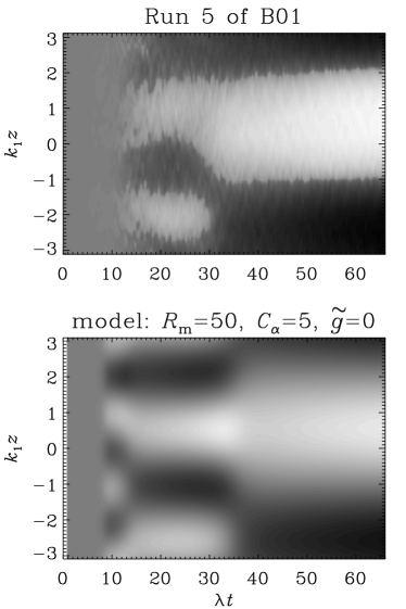
Figure 3: Comparison of the space-time (or butterfly) diagram from Run 5 of B01 with that from the one-dimensional model. Dark (light) shades indicate negative (positive) values. $R_{\rm m}=50$, ${\cal D}=5$, $\tilde{g}=0$.

In order to test the dynamical quenching theory more quantitatively, it would be useful to produce new simulations with smaller scale separation, e.g. $k_{\rm f}=2\ldots 3$, and an initial seed magnetic field where only one of several possible large scale eigenfunctions are present.

5.3 $\alpha^{2}\Omega$ dynamos: a parameter study

Table 1: The effect of changing $C_{\alpha}$ and $C_{\Omega}$ in an $\alpha^{2}\Omega$ dynamo with dynamical $\alpha$ quenching using the one-mode approximation. For all runs, $R_{\rm m}=20$, $\tilde{g}=0$.

$C_{\alpha}$	$C_{\Omega}$	$S/\eta k_{1}^{2}$	$b^{2}_{\rm fin}/B_{\rm eq}^{2}$	$B_{\rm fin}^{2}/B_{\rm eq}^{2}$	$Q^{-1}$	$\epsilon_{\rm m}$	$\omega_{\rm cyc}/S$	$\lambda/S$	remark
3.0	0	0	0.42	2.1	1.00	1.00	0	$2.0/C_{\Omega}$	$\alpha^{2}$ dynamo
3.0	2	42	0.48	3.4	0.58	0.71	0.36	1.1	$C_{\alpha}/C_{\Omega}={\cal O}(1)$
3.0	20	420	0.59	16	0.11	0.12	0.079	0.27	larger $C_{\Omega}$
1.0	20	420	0.19	9.5	0.071	0.10	0.050	0.12	smaller $C_{\alpha}$
0.3	20	420	0.042	2.1	0.071	0.10	0.050	0.045	smaller $C_{\alpha}$
0.1	20	420	0	0	0.071	0.100	0.050	0	marginal case
0.1	200	4200	0.019	9.5	0.007	0.010	0.005	0.012	same $C_{\alpha}C_{\Omega}$ as in line 3

When shear is included ($C_{\Omega}\neq 0$), toroidal field can be regenerated solely by the $S$-term in Eq. (56). When $C_{\Omega}\gg C_{\alpha}$, the dynamo efficiency is governed by the product $C_{\alpha}C_{\Omega}$. This is the regime where dynamical and fixed-form algebraic quenching lead to very different behaviors.

In order to study the effect of changing various input parameters we begin with Table 1 where we show the results for different values of $C_{\alpha}$. Note that only for small values of $C_{\alpha}$ do the results for $\epsilon_{\rm m}$ and $\omega_{\rm cyc}/S$ agree with the prediction of §4.2. This is simply because the $\alpha\Omega$ approximation made in §4.2 is only valid for $C_{\alpha}\ll C_{\Omega}$. As $C_{\alpha}$ increases, the field strength increases approximately as predicted by Eq. (30).

Increasing the value of $R_{\rm m}$ has no effect on the field geometry and time scales ($Q^{-1}$, $\epsilon_{\rm m}$, and $\lambda$ are unaffected); see Table 2. The field strength changes only when $R_{\rm m}$ is close to unity. Once $R_{\rm m}$ is above a certain value, the results are essentially independent of $R_{\rm m}$. For $\tilde{g}>0$, the field strength generally increases, as expected, and the cycle frequency decreases; see Table 3. One can also verify that $\epsilon_{\rm m}$ decreases as $\tilde{g}$ is increased. Models where $\eta_{\rm t}\propto\alpha$ (case II) tend to produce long cycle periods if the dynamo is sufficiently supercritical; see Table 4.

Table 2: Effect of changing $R_{\rm m}$ for two different values of $C_{\alpha}$ in the one-mode approximation. The increase of small and large scale field strength for small values of $R_{\rm m}$ is explained by the large values of $\iota$. For all the models with $C_{\alpha}=1.0$ we find $Q^{-1}=0.021$, $\epsilon_{\rm m}=0.014$, $\omega_{\rm cyc}/S=0.015$, $\lambda/S=0.045$, whilst for all the models with $C_{\alpha}=0.1$ we find $Q^{-1}=0.005$, $\epsilon_{\rm m}=0.007$, $\omega_{\rm cyc}/S=0.003$, $\lambda/S=0.011$. For all runs, $C_{\Omega}=300$, $\tilde{g}=0$, and $S/\eta k_{1}^{2}\equiv\iota R_{\rm m}C_{\Omega}$ varies between $6\times 10^{2}$ and $3\times 10^{5}$.

$R_{\rm m}$	$C_{\alpha}$	$b^{2}_{\rm fin}/B_{\rm eq}^{2}$	$B^{2}_{\rm fin}/B_{\rm eq}^{2}$
1000	1.0	0.19	15
100	1.0	0.19	15
10	1.0	0.21	17
1	1.0	0.38	30
100	0.1	0.019	13
10	0.1	0.021	15
1	0.1	0.037	28

Table 3: Effect of changing $\tilde{g}$ in the one-mode approximation. For all runs, $R_{\rm m}=20$, $C_{\alpha}=0.1$, $C_{\Omega}=200$, $S/\eta k_{1}^{2}=4200$, $b^{2}_{\rm fin}/B_{\rm eq}^{2}=0.02$, $\lambda/S=0.012$.

$\tilde{g}$	$B_{\rm fin}^{2}/B_{\rm eq}^{2}$	$Q^{-1}$	$\epsilon_{\rm m}$	$\omega_{\rm cyc}/S$
0	9.5	0.007	0.010	0.0050
0.3	24	0.0031	0.0043	0.0021
1.0	70	0.0011	0.0015	0.0010

Table 4: Effect of changing $C_{\Omega}$ for case II in the one-mode approximation. The critical value for dynamo action is $C_{\Omega}=20$. For all runs, $R_{\rm m}=20$, $C_{\alpha}=0.1$, $b^{2}_{\rm fin}/B_{\rm eq}^{2}=0.02$,

$C_{\Omega}$	$B_{\rm fin}^{2}/B_{\rm eq}^{2}$	$Q^{-1}$	$\epsilon_{\rm m}$	$\omega_{\rm cyc}/S$
22	31	0.0032	0.0045	0.0023
30	43	0.0023	0.0033	0.0017
50	75	0.0014	0.0019	0.0010
100	161	0.0007	0.0010	0.0005

5.4 A two-dimensional $\alpha^{2}\Omega$ dynamo

In order to compare with the simulations of BBS, it is important to consider the appropriate geometry and shear profile. As in BBS we use sinusoidal shear, $\overline{\bf{U}}=(0,Sk_{1}^{-1}\cos k_{1}x,0)$, and the mean field is $\overline{\bf{B}}=\overline{\bf{B}}(x,z,t)$; cf. §3. The results are shown in Table 5. The calculations have been carried out using a sixth order finite difference scheme in space and a third order Runge-Kutta scheme in time.

Table 5: Results from the two-dimensional $\alpha^{2}\Omega$ dynamo with dynamical $\alpha$ quenching. In the last two rows, the results from the simulations of BBS and BDS are given for comparison. Models AG2 and perhaps also R1 show some tentative agreement with BBS; the corresponding numbers are shown in bold face. Models s3 and S1 give some tentative agreement with BDS (where $S/\eta k_{1}^{2}=1000$); the corresponding numbers are shown in italics.

	$R_{\rm m}$	$C_{\alpha}$	$C_{\Omega}$	$\tilde{g}$	$S/\eta k_{1}^{2}$	$b^{2}_{\rm fin}/B_{\rm eq}^{2}$	$B^{2}_{\rm fin}/B_{\rm eq}^{2}$	$Q^{-1}$	$\epsilon_{\rm m}$	$\omega_{\rm cyc}/S$	$\lambda/S$
A1	20	0.3	100	0	2000	0.05	4.0	0.032	0.068	0.015	0.018
A2	20	1.0	100	0	2000	0.20	15	0.031	0.065	0.016	0.046
A3	20	3.0	100	0	2000	0.62	48	0.031	0.064	0.015	0.098
R1	20	1.0	100	0	2000	0.20	15	0.031	0.065	0.016	0.044
R2	50	1.0	40	0	2000	0.17	5.5	0.076	0.16	0.035	0.055
R3	100	1.0	20	0	2000	0.14	2.3	0.15	0.30	0.072	0.061
G1	20	0.3	100	0	2000	0.05	4.0	0.032	0.068	0.015	0.018
G2	20	0.3	100	0.1	2000	0.05	5.2	0.025	0.053	0.011	0.018
G3	20	0.3	100	0.3	2000	0.06	8.2	0.018	0.036	0.009	0.018
G4	20	0.3	100	1.0	2000	0.06	23	0.007	0.014	0.007	0.018
G5	20	0.3	100	3.0	2000	0.06	56	0.003	0.006	0.0013	0.018
AG1	100	0.3	20	3.0	2000	0.00	0	–	–	–	0
AG2	100	0.5	20	3.0	2000	0.10	22	0.011	0.024	0.006	0.021
AG3	100	1.0	20	3.0	2000	0.20	70	0.007	0.015	0.004	0.052
s1	30	0.25	33	1.0	1000	0.05	3	0.035	0.072	0.017	0.007
s2	30	0.30	33	1.0	1000	0.06	4	0.032	0.066	0.015	0.012
s3	30	0.35	33	1.0	1000	0.07	6	0.029	0.061	0.014	0.016
S1	30	0.35	33	3.0	1000	0.07	19	0.009	0.019	0.005	0.016
S2	50	0.35	20	3.0	1000	0.07	10	0.017	0.035	0.008	0.006
S3	50	0.4	20	3.0	1000	0.08	14	0.015	0.031	0.006	0.011
S4	100	0.4	20	3.0	2000	0.08	14	0.014	0.028	0.008	0.011
BDS	$\sim 30$	1–2	–	–	1000	4	20	0.018	0.11	0.013–0.015	0.006
BBS	$\sim 80$	1–2	–	–	2000	6	30	0.014	0.06	0.005–0.010	0.015

Figure 4: Space-time (or butterfly) diagram of ${\overline{B}}_{y}$ for Model S1 with dynamical quenching. At $x=-\pi$ ($x=0$) the shear has attained and negative (positive) maximum. Dark (light) shades indicate negative (positive) values. $R_{\rm m}=30$, $C_{\alpha}=0.35$, $C_{\Omega}=33$, $\kappa_{\rm f}=5$, $\epsilon_{\rm f}=1$, $\tilde{g}=3$.

As in the simulations of BBS, we have chosen negative values of $\alpha_{\rm K}$, but this choice only affects the direction of propagation of the dynamo waves. There are dynamo waves traveling in the positive $z$-direction at $x=\pm\pi$ and in the negative $z$-direction at $x=0$, which is consistent with the three-dimensional simulations. These waves are best seen in a space-time (or butterfly) diagram; see Fig. 4. Note also that there is an initial adjustment time during which the overall magnetic energy settles onto its final value (consistent with resistively limited saturation) and the cycle period increases by a small amount.

Compared with the one-dimensional model, the values of $Q^{-1}$ and $\epsilon_{\rm m}$ are about 30% larger in the two-dimensional model, but $\omega_{\rm cyc}$ is about 3 times smaller. This may reflect the fact that in the present geometry the upward and downward traveling dynamo waves can propagate less freely, because they are now also coupled in the $x$ direction.

For comparison, in the simulation of BBS, the inferred input parameters for modeling purposes are $k_{\rm m}^{2}=2$ (the field varies in $x$ and $z$), $S/\eta k_{1}^{2}=2000$, $R_{\rm m}\approx u_{\rm rms}/\eta k_{\rm f}\approx 80$, $C_{\alpha}\approx\tilde{\kappa}_{\rm f}=1...2$. The resulting non-dimensional output quantities are $B^{2}_{\rm fin}/B_{\rm eq}^{2}\approx 30$, $Q^{-1}\approx 0.02$, $\epsilon_{\rm m}\approx 0.11$, $\omega_{\rm cyc}/S=0.005\dots 0.010$, and $\lambda/(\eta k_{\rm m}^{2})=30$.

Figure 5: Evolution of the large scale magnetic energy for Model AG2 (solid line). The dotted line gives the comparison with the corresponding adiabatic approximation (see appendix A). $R_{\rm m}=100$, $C_{\alpha}=0.5$, $C_{\Omega}=20$, $\kappa_{\rm f}=5$, $\epsilon_{\rm f}=1$, $\tilde{g}=3$.

Model R1 gives, within a factor of two, about the right saturation field strength, and also the values of $Q^{-1}$, $\epsilon_{\rm m}$ and $\omega_{\rm cyc}/S$ agree reasonably well with the simulations, but the kinematic growth rate is too high. Also, the value of $R_{\rm m}$ is probably larger in the simulation where we estimated $R_{\rm m}\approx 80$. In order to have the right growth rate, $C_{\alpha}$ has to be lowered. In order to match then the right saturation field strength we have to have $\tilde{g}\approx 3$. One such case is Model AG2, where $R_{\rm m}=100$. Now cycle frequency, growth rate, as well as $Q^{-1}$ agree reasonably well with the simulation.

The simulation of BDS is more resistive, $S/\eta k_{1}^{2}=1000$ and $R_{\rm m}\approx 30$, but the resulting field strength is only somewhat smaller, $B^{2}_{\rm fin}/B_{\rm eq}^{2}\approx 20$, whereas $Q^{-1}\approx 0.02$, $\epsilon_{\rm m}\approx 0.11$ and $\omega_{\rm cyc}/S=0.013\dots 0.015$ are all somewhat enhanced relative to BBS. Models s1…s3 (where $\tilde{g}=1$) and S1…S3 (where $\tilde{g}=3$) are now appropriate for comparison, because they all have $S/\eta k_{1}^{2}=1000$. Model S1 with $\tilde{g}=3$ gives the best agreement for $B^{2}_{\rm fin}$, but the cycle frequency is too small. For Model s3 with $\tilde{g}=1$, $\omega_{\rm cyc}$ is about right, but now $B^{2}_{\rm fin}$ is too small.

In all models the values of $b^{2}_{\rm fin}$ in table 5 are smaller than in the simulations. As discussed in §4.1, this is readily explained by the fact that our model does not take into account small scale dynamo action resulting from the non-helical component of the flow.

Comparing the two simulations with different values of $R_{\rm m}$ (BBS and BDS), the cycle frequency changes by a factor compatible with the ratio of the two magnetic Reynolds numbers. This is not well reproduced by a quenching expression for $\eta_{\rm t}$ that is independent of $R_{\rm m}$ (case I). On the other hand, if $\eta_{\rm t}\propto\alpha$ (case II), $\omega_{\rm cyc}$ becomes far smaller than what is seen in the simulations. A possible remedy would be to have some intermediate quenching expression for $\eta_{\rm t}$. We should bear in mind, however, that our current model ignores the feedback from the large scale motions. Such feedback is indeed present in the simulations, which also show much more chaotic behavior (e.g. Fig. 8 of BBS) than our model; see Fig. 5. A more realistic model should therefore allow for more degrees of freedom. In particular, the quenching should be allowed to be nonuniform in space. This and other extensions of the model are discussed in the next section.

6 Possible extensions of the model

The dynamical quenching model allows us now to test a number of additional aspects and properties that have been (or can be) seen in direct simulations.

6.1 Cross helicity evolution and large scale velocity feedback

Although we were justified in ignoring the small scale cross helicity contribution to ${\cal E}$, we found from the simulation of BBS that the large scale cross helicity is non-negligible. This turned out to be the result of the forcing function for the large scale velocity and the asymmetry of the large scale field with respect to $x=0$, and thus with respect to the large scale velocity. The correlation between the forcing function for the large scale flow and the large scale magnetic field serves as a driver in the cross helicity evolution equation. In principle, we should explicitly couple the equation for the cross helicity into the model. Our models with imposed shear, however, did not produce the required symmetry breaking that would lead to a significant contribution to the large scale cross helicity. This is because we treat the large scale velocity as being kinematic. This should be explored further in future work by accounting for the dynamical feedback from the large scale motions.

6.2 Antiquenching

As long as the feedback from the small scale motions onto $\alpha$ and $\eta_{\rm t}$ involve the quantity $\langle{\bf{a}}\cdot{\bf{b}}\rangle$, i.e. as long as Eqs (4) and (5) remain fully coupled, Eq. (2) is guaranteed to be satisfied. Thus, the magnetic helicity equation is obeyed regardless of how $\langle{\bf{a}}\cdot{\bf{b}}\rangle$ is coupled to $\alpha$ or $\eta_{\rm t}$. It may be that under certain conditions, $\alpha$ and $\eta_{\rm t}$ may even increase with increasing field strength, which we refer to as ‘anti-quenching’. Brandenburg, Saar, & Turpin (1998) used such models to explain the increase of relative stellar cycle frequency with increasing field strength. As an illustrative example, we have considered the case $\alpha=\alpha_{\rm K}-\alpha_{\rm M}$, i.e. with the opposite sign as in Eq. (7), and $\eta_{\rm t}=\eta_{\rm t0}(1+\langle{\bf{b}}^{2}\rangle^{2}/B_{\rm eq}^{2})$, where $\langle{\bf{b}}^{2}\rangle$ is linked to $\langle{\bf{a}}\cdot{\bf{b}}\rangle$ via Eqs (24) and (26). Note that $\eta$ antiquenching goes with the 4th power, so that it eventually dominates over $\alpha$ antiquenching. The resulting evolution of $\langle\overline{\bf{B}}^{2}\rangle$ shows the expected resistively limited saturation phase. Alternatively, if $\alpha$ is made to increase with increasing small scale field strength, the resulting large scale field can saturate faster than usual. A similar behavior can be modeled by choosing $\tilde{g}<0$, which also speeds up the initial build-up of large scale magnetic energy. This is possible, and consistent with the magnetic helicity equation, because the initial build-up of $\langle\overline{\bf{B}}^{2}\rangle$ happens in this case simultaneously with a sharp burst in $\langle{\bf{b}}^{2}\rangle$ such that the sum of $\langle\overline{\bf{A}}\cdot\overline{\bf{B}}\rangle$ and $\langle{\bf{a}}\cdot{\bf{b}}\rangle$ is still approximately constant.

6.3 Magnetic buoyancy

In solar and galactic dynamo theory the possibility of rising magnetic flux tubes contributing to the $\alpha$ effect has been discussed (Leighton 1969; Ferriz-Mas, Schmitt, & Schüssler 1994; Hanasz & Lesch 1997; Brandenburg & Schmitt 1998; Moss, Shukurov, & Sokoloff 1999; Thelen 2000; Spruit 2002). For the sun, the idea is that flux tubes emerge from the toroidal magnetic field belt at the bottom of the convection zone and become twisted by the Coriolis force. We point out that Eq. (18) does already capture part of this effect. If there is a strong partly buoyant magnetic field at the bottom of the convection zone, it would contribute to $\langle\overline{\bf{J}}\cdot\overline{\bf{B}}\rangle$ and therefore, through Eq. (18), to $\alpha$. Of course, this effect cannot constitute a dynamo on its own as there is no source of magnetic energy. However, in conjunction with shear, from which energy can be tapped, this effect could lead to dynamo action. Modeling this in the framework of dynamical quenching would be a suitable way to include the effects of magnetic buoyancy such that magnetic helicity conservation is obeyed.

6.4 Oscillatory imposed fields

If there is a uniformly imposed magnetic field that is oscillatory in time, Eq. (18) would predict that $\alpha$ is also oscillatory. If the oscillation frequency is high enough, the adiabatic approximation breaks down. One might wonder whether this would be a way to test explicitly the dynamical $\alpha$ quenching concept numerically. However, it turns out that the resulting averaged $\alpha$ is even smaller on average than what is predicted based on the adiabatic approximation. Thus, although dynamical quenching enhances dynamo generation in the case of self-generated fields, it actually lowers $\alpha$ in the presence of imposed oscillatory fields.

6.5 Selective decay

In is interesting to note that Eq. (18) can also be applied to the case of decaying magnetic fields. In that case, it predicts reduced turbulent decay if $\langle\overline{\bf{J}}\cdot\overline{\bf{B}}\rangle\neq 0$. Thus, accordingly, a fully helical magnetic field should only decay at the resistive rate, whereas a non-helical magnetic field would decay at the turbulent diffusive rate. The slow decay of helical fields is well known and leads to the so-called Taylor states where magnetic helicity is maximized and magnetic energy minimized (e.g. Montgomery, Turner, & Vahala 1978).

6.6 Hyperdiffusion

Numerical experiments allow one to understand the physics described by the equations by modifying certain terms. Particularly enlightening has been the use of hyperresistivity (or hyperdiffusion) by which the ordinary diffusion operator, $\eta\nabla^{2}$, is simply replaced by $\eta_{2}\nabla^{4}$. The diffusion at small scales is usually fixed by the mesh resolution and kept unchanged, but with hyperdiffusion the diffusion at large scales can be decreased substantially. This method is frequently used in turbulence research, but the effects on helical dynamos are quite striking: the saturation field strength is considerably enhanced and the saturation phase prolonged (Brandenburg & Sarson 2002). Our model reproduces these features if $\eta k_{\rm f}^{2}$ is replaced by $\eta_{2}k_{\rm f}^{4}$, $\eta\overline{\bf{J}}$ is replaced by $-\eta_{2}\nabla^{2}\overline{\bf{J}}$, and $R_{\rm m}=\eta_{\rm t}/(\eta_{2}k_{\rm f}^{3})$ is used. The simulations of Brandenburg & Sarson (2002) showed (for the helical dynamo without shear) that the large scale field behavior depends on the diffusion at the scale of the large scale field itself and not, as one might naively expect, on the diffusion at small scales. This behavior is clearly reproduced by the dynamical quenching model: reducing the microscopic $\eta$ in the mean field equation (and not in the dynamical quenching equation) increases saturation time and saturation value as expected. This can be taken as additional validation of the dynamical quenching model.

6.7 Losses of small scale field

Open boundaries may provide a means of shedding magnetic helicity and thereby alleviating the magnetic helicity constraint (Blackman & Field 2000; Kleeorin et al. 2000; 2002). Numerical simulations have shown, however, that when no additional boundary physics is imposed to transport preferentially quantities of a particular scale, most of the magnetic helicity is lost by the large scale field (Brandenburg & Dobler 2001). In this case, the growth of the large scale field cannot be accelerated. In order to check whether accelerated growth of large scale fields is at least in principle possible we have modeled the preferential shedding of small scale fields in two different ways, both with similar results. Adding an overall loss term of the form $-\alpha_{\rm M}/\tau_{\rm loss}$ on the right hand side of Eq. (18) leads to substantial increase of the large scale field [note that this is distinct from the $-\alpha_{\rm M}/T$ in Kleeorin et al. (2000), which is just the same as our second term in Eq. (13)]. Likewise, setting $\langle{\bf{b}}^{2}\rangle$ (and hence $\alpha_{\rm M}$) to zero in sporadic intervals accelerates the growth phase and enhances the saturation value. Similar results have meanwhile also been obtained by restarting Run 3 of B01 after sporadically removing magnetic field at and below the forcing scale (see Fig. 14 of BDS). This confirms an important prediction from the dynamical quenching model.

6.8 Generalization to nonuniform $\alpha$

Our approach is based on magnetic helicity which is a volume integral. However, in astrophysical bodies kinetic and magnetic helicities are not spatially constant and change sign at the equator. Generalizing Eq. (13) to the case of space dependent $\alpha_{\rm K}$ and $\alpha_{\rm M}$ seems at first glance straightforward: omit the angular brackets and replace ${\rm d}{}/{\rm d}{}t$ by $\partial/\partial t$, as was done already in the early work of Kleeorin & Ruzmaikin (1982). It may also be necessary to include a local phenomenological magnetic helicity flux transport term, for example of the form $\eta_{\alpha}\nabla^{2}\alpha_{\rm M}$ (in addition to whatever global flux terms may be present, e.g. Blackman & Field 2000; Kleeorin et al. 2002). In the presence of large scale (meridional) flows, it may furthermore be appropriate to use the advective derivative, ${\rm D}{}/{\rm D}{}t=\partial/\partial t+\overline{\bf{U}}\cdot\mbox{\boldmath$\nabla$}{}$. However, the magnetic helicity density, ${\bf{a}}\cdot{\bf{b}}$, is not gauge-invariant and it is no longer strictly related to ${\bf{j}}\cdot{\bf{b}}$ locally. The hope would be that the generalization outlined above may still be useful as an approximation.

We have performed calculations with $\alpha_{\rm K}=\alpha_{\rm K0}\sin k_{1}z$ and $C_{\alpha}\equiv\alpha_{\rm K0}/(\eta_{\rm T}k_{1})=5$. The resulting large scale field strength is approximately equal to $B_{\rm eq}$, and depends only weakly on $R_{\rm m}$. This is consistent with Kleeorin et al. (2002). Simulations with the same sinusoidal $\alpha$ profile (Brandenburg 2001b) have shown that the resulting large scale field varies mostly in the $x$ direction, which is incompatible with the present model. Also the resulting field strength was actually significantly below $B_{\rm eq}$.

In the presence of open boundaries the present model predicts large scale field strengths that decrease inversely proportional with $R_{\rm m}$. This is even steeper that what was found in the simulations (Brandenburg & Dobler 2001). Thus, in its present form the dynamical quenching model does not reproduce satisfactorily the numerical results when $\alpha$ varies in space. However, with the help of simulations it should be possible to identify which of the steps in the derivation of dynamical $\alpha$ quenching are no longer satisfied, and hence what the cause of the problem is.

7 Conclusions

The magnetic helicity evolution equation is a constraint that must be satisfied by any dynamo theory. When we apply this in the mean field formalism with the prescription that the $\alpha$ effect is proportional to the difference between kinetic and current helicities, dynamical $\alpha$ quenching emerges as the only theoretically consistent approach to $\alpha$ quenching. This is supported by comparisons with numerical simulations of dynamos with and without shear. Fixed-form, algebraic quenching prescriptions may apply in a specific parameter regime (e.g. the saturated phase), but are invalid for earlier times and are inconsistent with results from time dependent analyses. Only dynamical quenching has predictive power.

A key result from dynamical quenching is that near-equipartition large scale field strengths are reached independently of the magnetic Reynolds number by the end of the kinematic phase. Final saturation is only reached on a resistively limited ($R_{\rm m}$ dependent) time scale but with a saturation value independent of $R_{\rm m}$ and equal to $B_{\rm fin}^{2}/B_{\rm eq}^{2}=\tilde{k}_{\rm f}/\tilde{k}_{\rm m}$; see Eqs (30) and (32).

Although magnetic helicity conservation provides a basis for a dynamical quenching of $\alpha$, the form of $\eta_{\rm t}$ must be prescribed at present. We have shown that current simulations of $\alpha^{2}$ (shear-free) dynamos constrain the dynamical quenching of $\overline{\mbox{\boldmath${\cal E}$}}{}\cdot{\overline{\bf B}}$ which is a combination of $\alpha$ and $\eta_{\rm t}$, but they do not separately constrain $\eta_{\rm t}$. On the other hand, cycle periods, emerging only in dynamos with shear, can. At present, the shear dynamo simulations are best described by a dynamical quenching theory in which $\eta_{\rm t}$ is only weakly dependent on the magnetic field; $\tilde{g}\approx 3$ in Eq. (15). Higher resolution simulations are needed to verify this.

The two-scale dynamical nonlinear quenching approach based on magnetic helicity conservation discussed herein constitutes an improvement over fixed-form algebraic quenching approaches. Nevertheless, there are aspects of high-Reynolds number $\alpha\Omega$ dynamos that may require the theory to be augmented. For example, we have only considered a spatially uniform $\alpha$ coefficient. Allowing for spatial gradients in $\alpha$ will introduce local helicity flux terms that are important for astrophysical bodies where $\alpha$ changes sign across the equator. In addition, helicity flux across global boundaries was also ignored in our calculation, though we know that real systems have boundaries. The associated boundary magnetic helicity flow may be important in coupling the dynamo growth to magnetic helicity evolution.

Appendix A The adiabatic approximation

We discuss here the justification for when the time derivative in the dynamical quenching expression can be neglected (the adiabatic approximation).

In the steady state, $\alpha_{\rm M}$ and $\langle\overline{\bf{B}}^{2}\rangle$ are given by Eqs (29) and (30), respectively. Linearizing Eqs (17) and (18) about this state yields

$${\textstyle{1\over 2}}{{\rm d}{}\mbox{\boldmath$q$}{}\over{\rm d}{}t}=\pmatrix{-(\alpha_{\rm K}/\tilde{k}_{\rm m}-\eta_{\rm t})k_{\rm f}^{2}&\eta k_{\rm f}^{2}\cr-(\alpha_{\rm K}/\tilde{k}_{\rm m}-\eta_{\rm T}\!)k_{\rm m}^{2}&0}\mbox{\boldmath$q$}{},$$ (A1)

where $\mbox{\boldmath$q$}{}\equiv\left(\delta\!\ln\alpha_{\rm M},\,\delta\!\ln\langle\overline{\bf{B}}^{2}\rangle\right)$ is the state vector for the logarithmic departure from equilibrium. For excited solutions, the terms in the first column of the matrix in (A1) are usually positive, even for $\alpha\Omega$ dynamos. Inspecting the diagonal terms shows that near the saturated state, $\alpha_{\rm M}$ is adjusting rapidly on a dynamical time scale whilst $\langle\overline{\bf{B}}^{2}\rangle$ is marginal and adjusts only indirectly (via $\alpha_{\rm M}$) on a resistive time scale. We can therefore use the adiabatic elimination principle (e.g. Haken 1983) to remove the explicit time dependence of $\alpha_{\rm M}$ by replacing Eq. (18) by

$$0=\left(\alpha\langle\overline{\bf{B}}^{2}\rangle-\eta_{\rm t}\mu_{0}\langle\overline{\bf{J}}\cdot\overline{\bf{B}}\rangle\right)/B_{\rm eq}^{2}+\alpha_{\rm M}/R_{\rm m}.$$ (A2)

Substituting $\alpha_{\rm M}=\alpha-\alpha_{\rm K}$ and solving for $\alpha$ leads to Eq. (40).

The adiabatic approximation corresponds to the limit in which memory effects become negligible. This is best seen by considering the integral form of Eq. (18),

$$\alpha=2\eta k_{\rm f}^{2}\int_{0}^{\displaystyle{t}}G(t,t^{\prime})\left(\alpha_{\rm K}+R_{\rm m}\eta_{\rm t}\mu_{0}{\langle\overline{\bf{J}}\cdot\overline{\bf{B}}\rangle\over B_{\rm eq}^{2}}\right){\rm d}{}t^{\prime},$$ (A3)

with the Green’s function

$$G(t,t^{\prime})=\exp\left[-2\eta k_{\rm f}^{2}\int_{\displaystyle{t^{\prime}}}^{\displaystyle{t}}\left(1+R_{\rm m}{\langle\overline{\bf{B}}^{2}\rangle\over B_{\rm eq}^{2}}\right){\rm d}{}t^{\prime\prime}\right].$$ (A4)

As long as the field is weak, the width of the Green’s function is the resistive time scale, but when $\langle\overline{\bf{B}}^{2}\rangle/B_{\rm eq}^{2}$ is of order unity the large $R_{\rm m}$ factor becomes important and the width of the Green’s function reduces to a dynamical time scale. In that case, the $\overline{\bf{B}}$ dependent terms in brackets can be pulled out of the integrals in Eqs (A3) and (A4), in which case Eq. (40) is recovered.

References

- (1) Bhattacharjee, A., & Yuan, Y. 1995, ApJ, 449, 739
- (2) Blackman, E. G., & Field, G. F. 2000, ApJ, 534, 984
- (3) Brandenburg, A. 2001a, ApJ, 550, 824 (B01)
- (4) Brandenburg, A. 2001b, astro-ph/0011579
- (5) Brandenburg, A., & Dobler, W. 2001, A&A, 369, 329
- (6) Brandenburg, A., & Sarson, G. R. 2002, PRL, 88, 055003-1 (BS02)
- (7) Brandenburg, A., & Schmitt, D. 1998, A&A, 338, L55
- (8) Brandenburg, A., Bigazzi, A., & Subramanian, K. 2001, MNRAS, 325, 685 (BBS)
- (9) Brandenburg, A., Dobler, W., & Subramanian, K. 2002, AN, 323, 99 (BDS) astro-ph/0111567
- (10) Brandenburg, A., Saar, S. H., & Turpin, C. R. 1998, ApJ, 498, L51
- (11) Brandenburg, A., Nordlund, Å., Stein, R. F., & Torkelsson, U. 1995, ApJ, 446, 741
- (12) Brandenburg, A., Jennings, R. L., Nordlund, Å., Rieutord, M., Stein, R. F., & Tuominen, I. 1996, JFM, 306, 325
- (13) Cattaneo, F., & Vainshtein, S. I. 1991, ApJ, 376, L21
- (14) Cattaneo, F., & Hughes, D. W. 1996, Phys. Rev., E 54, R4532
- (15) Covas, E., Tworkowski, A., Brandenburg, A., & Tavakol, R. 1997, A&A, 317, 610
- (16) Covas, E., Tavakol, R., Tworkowski, A., & Brandenburg, A. 1998, A&A, 329, 350
- (17) Covas, E., Tavakol, R., Tworkowski, A., Brandenburg, A., Brooke, J., & Moss, D. 1999, A&A, 345, 669
- (18) Ferriz-Mas, A., Schmitt, D., & Schüssler, M. 1994, A&A, 289, 949
- (19) Feudel, U., Jansen, W., Kurths, J. 1993, J. Bifurcation & Chaos, 3, 131
- (20) Field G. B., & Blackman E. G. 2002, ApJ, 572, 685 (FB02)
- (21) Gruzinov, A. V., & Diamond, P. H. 1994, PRL, 72, 1651
- (22) Gruzinov, A. V., & Diamond, P. H. 1995, Phys. Plasmas, 2, 1941
- (23) Gruzinov, A. V., & Diamond, P. H. 1996, Phys. Plasmas, 3, 1853
- (24) Haken, H. 1983, Synergetics – An Introduction (Springer, Berlin), 3rd edition, Chap. 7.2
- (25) Hanasz, M. & Lesch, H. 1997, A&A, 321, 1007
- (26) Ji, H. 1999, PRL, 83, 3198
- (27) Kitchatinov, L. L., Rüdiger, G., & Pipin, V. V. 1994, AN, 315, 157
- (28) Kleeorin, N. I., & Ruzmaikin, A. A. 1982, Magnetohydrodynamics, 2, 17
- (29) Kleeorin, N. I, Rogachevskii, I., & Ruzmaikin, A. 1995, A&A, 297, 159
- (30) Kleeorin, N., & Rogachevskii, I. 1999, Phys. Rev., E 59, 6724
- (31) Kleeorin, N. I, Moss, D., Rogachevskii, I., & Sokoloff, D. 2000, A&A, 361, L5
- (32) Kleeorin, N., Moss, D., Rogachevskii, I., & Sokoloff, D. 2002, A&A, 387, 453
- (33) Krause, F., & Rädler, K.-H. 1980, Mean-Field Magnetohydrodynamics and Dynamo Theory (Akademie-Verlag, Berlin; also Pergamon Press, Oxford)
- (34) Kulsrud, R. M., & Anderson, S. W. 1992, ApJ, 396, 606
- (35) Leighton, R. B. 1969, ApJ, 156, 1
- (36) Moffatt, H. K. 1978, Magnetic Field Generation in Electrically Conducting Fluids (Cambridge University Press, Cambridge)
- (37) Moss, D., Shukurov, A., & Sokoloff, D. 1999, A&A, 343, 120
- (38) Montgomery, D., Turner, L., & Vahala, G. 1978, Phys. Fluids, 21, 757
- (39) Nordlund, Å., Galsgaard, K., & Stein, R. F. 1994, in Solar surface magnetic fields, ed. R. J. Rutten & C. J. Schrijver (NATO ASI Series, Vol. 433), 471
- (40) Parker, E. N. 1979, Cosmical Magnetic Fields (Clarendon Press, Oxford)
- (41) Pouquet, A., Frisch, U., & Léorat, J. 1976, JFM, 77, 321
- (42) Robinson, R. D., & Durney, B. R. 1982, A&A, 108, 322
- (43) Rogachevskii, I. & Kleeorin, N. 2001, Phys. Rev., E 64, 056307
- (44) Rüdiger, G., & Kitchatinov, L. L. 1993, A&A, 269, 581
- (45) Ruzmaikin, A. A. 1981, Comments Astrophys., 9, 85
- (46) Schmalz, S., & Stix, M. 1991, A&A, 245, 654
- (47) Seehafer, N. 1996, Phys. Rev., E 53, 1283
- (48) Spruit, H. C. 2002, A&A, 381, 923
- (49) Subramanian, K. 2002, Bull. Astr. Soc. India, (in press), astro-ph/0204450
- (50) Thelen, J.-C. 2000, MNRAS, 315, 165
- (51) Vainshtein, S. I., & Cattaneo, F. 1992, ApJ, 393, 165
- (52) Yoshimura, H. 1978, ApJ, 226, 706
- (53) Yoshizawa, A., & Yokoi, N. 1993, ApJ, 407, 540
- (54) Zeldovich, Ya. B., Ruzmaikin, A. A., & Sokoloff, D. D. 1983, Magnetic Fields in Astrophysics (Gordon & Breach, New York)