Supernova 1998bw - The final phases

The probable association with GRB~980425 immediately put SN~1998bw at the forefront of supernova research. Here, we present revised late-time $BVRI$ light curves of the supernova, based on template images taken at the VLT. To follow the supernova to the very last observable phases we have used HST/STIS. Deep images taken in June and November 2000 are compared to images taken in August 2001. The identification of the supernova is firmly established. This allows us to measure the light curve to $\sim 1000$ days past explosion. The main features are a rapid decline up to more than 500 days after explosion, with no sign of complete positron trapping from the $\@element[56]{\mathrm{Co}}$ decay. Thereafter, the light curve flattens out significantly. One possible explanation is powering by more long lived radioactive isotopes, if they are abundantly formed in this energetic supernova.

1 Introduction

Supernova (SN) 1998bw was discovered in April 1998 in a spiral arm of the face-on SB galaxy ESO~184-G82 at a redshift of $z=0.0085$ (Galama et al. 1998a). This exceptional type Ic supernova was born famous because of its positional and temporal coincidence with the gamma-ray burst GRB~980425 (Galama et al. 1998b). This association was further supported by the very early onset of the bright radio luminosity (Kulkarni et al. 1998). Also in the optical, the supernova was unusually luminous and showed very high expansion velocities (Patat et al. 2001).

The earliest photometric evolution of SN~1998bw was presented in Galama et al. (1998b). McKenzie & Schaefer (1999) monitored the early exponential decay, and the late phases were added by Sollerman et al. (2000). Patat et al. (2001) combined these data to make a rough bolometric light curve, which has been the basis of several model investigations (Nomoto et al. 2001; Nakamura et al. 2001a). The aim of this paper is to improve and extend this light curve to the final phases of SN~1998bw.

Modelling of the early light curve and spectra suggested an extremely energetic explosion [$(2-5)\times\leavevmode\nobreak\ 10^{52}$ erg] of a massive star, composed mainly of carbon and oxygen (Iwamoto et al. 1998; Woosley et al. 1999). As this kinetic energy is more than ten times that of a canonical core-collapse supernova, the term hypernova was suggested for this event. The mass of $\@element[56]{\mathrm{Ni}}$ needed to power the early light curve in these early models, 0.5–0.7 ${\leavevmode\nobreak\ \rm M}_{\odot}$, is much larger than the $\la 0.1$ ${\leavevmode\nobreak\ \rm M}_{\odot}$ typical for “normal” core-collapse SNe (e.g., Sollerman 2002).

This large mass of $\@element[56]{\mathrm{Ni}}$ was disputed by Höflich et al. (1999), who suggested that the early light curve could be reproduced by a normal SN Ic, given the right viewing angle and degree of asymmetry. The modelling of Sollerman et al. (2000) indicated, however, that at least 0.3 ${\leavevmode\nobreak\ \rm M}_{\odot}$ of $\@element[56]{\mathrm{Ni}}$ was required to power the late emission of the supernova. This conclusion was later supported by Nakamura et al. (2001a), see also Mazzali et al. (2001).

In this paper we focus on the very late light curve of SN~1998bw. In Sect. 2 we present new VLT observations and the technique used to achieve the revised optical light curves. Here we also present some late near-IR photometry. In Sect. 3 we present the very late Hubble Space Telescope (HST) observations of SN~1998bw. The results are presented in Sect. 4. After a discussion in Sect. 5, we briefly summarize our conclusions in Sect. 6.

2 Ground Based Observations

2.1 Late-Time Optical Photometry

The photometry discussed here is based on the late observations presented in Sollerman et al. (2000; hereafter S00). S00 obtained data at eight epochs between 32 and 503 days past explosion, using the ESO 3.6m telescope on La Silla and the Very Large Telescope (VLT) on Paranal. Here we assume the date of explosion to be 980425.9, the moment of detection of GRB~980425 (Soffitta et al. 1998).

To the S00 data set we have added the late time observations presented in Patat et al. (2001; hereafter P01). These data were primarily obtained using the ESO 3.6m telescope and are added in particular to include the $B$-band photometry. We have also added previously unpublished photometry obtained at the VLT. The details of the ground-based optical observations are shown in Table 1.

Table 1: Log of ground based observations

Date	MJDa	Epochb	Telescopec	Bands	Source
13 Sep. 98	1069	140	3.6m	$V\!RI$	S00
26 Nov. 98	1143	214	3.6m	$V\!RI$	S00
18 Mar. 99	1255	326	3.6m	$V\!RI$	S00
18 Mar. 99	1255	326	0.9m	$B$	P01
08 Apr. 99	1276	347	3.6m	$BV\!R$	P01
12 Apr. 99	1280	351	3.6m	$I$	P01
17 Apr. 99	1285	356	VLT	$V\!RI$	S00
17 Apr. 99	1285	356	VLT	$B$	This work
21 May 99	1319	390	3.6m	$BV\!RI$	P01
13 Jun. 99	1342	413	VLT	$V\!RI$	S00
17 Jun. 99	1346	417	3.6m	$BV\!RI$	P01
09 Aug. 99	1399	470	3.6m	$V\!RI$	S00
11 Sep. 99	1432	503	VLT	$V\!RI$	S00
11 Sep. 99	1432	503	VLT	$B$	This work
16 Oct. 99	1467	538	VLT	$BV\!RI$	This work
01 Apr. 00	1635	706	VLT	$BV\!RI$	This work
Oct./Nov. 00	$\sim 1836$	$\sim 907$	VLT	$BV\!RI$	This work

^a MJD$=$Julian Date$-$240000.5
^b Epoch in days past 980425.9
^c VLT=UT1+FORS1, 3.6m=ESO-3.6m+EFOSC2,
   0.9m=ESO-Dutch-0.92m

As discussed in S00 and P01, the photometry of SN~1998bw is fairly complicated. This is because the supernova is superposed on an H ii region, and sits in a rather complex region of the host galaxy. This was strikingly revealed by the HST/STIS image published by Fynbo et al. (2000), where several objects can be seen within $1\arcsec$ of the position of the supernova. This is here shown in detail in Fig. 1.

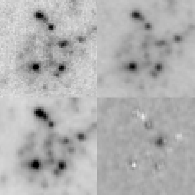
Figure 1: HST/STIS CLEAR images of SN~1998bw and its environment. The images were obtained in 2000 June (upper left), 2000 November (upper right), and 2001 August (lower left). The field of view is merely $1\aas@@fstack{\prime\prime}5\times 1\aas@@fstack{\prime\prime}5$. Lower right shows a subtraction between the first and the final frame. The supernova is clearly identified. The apparent differences in resolution are due to differences in the dithering procedure, as explained in the text.

This means that even sophisticated point-spread function (PSF) fitting photometry may not be adequate to accurately measure the SN brightness at late phases. S00 used DAOPhot to estimate the errors due to background subtraction, while P01 used the SNOOPY software. Although these methods were consistent, the very complex background of SN~1998bw as observed with HST called for a revision of the light curve. We decided to try another method to establish the late time light curve of this important supernova.

We therefore obtained deep $B$, $V$, $R$, and $I$ imaging of the region containing the supernova using FORS1 on the VLT. These observations were obtained in service mode under excellent atmospheric conditions in early October and in early November 2000, some 900 days after the supernova explosion. In each filter band 6–9 frames were coadded to achieve a deep combined image. The $B$ and $V$ frames have a total exposure time of 90 minutes each, while the $R$ and $I$ frames have 120 minutes. All combined frames have good image quality, with a FWHM less than one arcsecond.

In these images, no sign of the supernova could be detected, i.e., the background on the position of the supernova appeared smooth. These frames were therefore used as template frames to subtract the background from all the previous images (see e.g., Filippenko et al. 1986 for an early account of this method). The detailed procedure used is outlined in Schmidt et al. (1998), and we have used the same software as used by the High-$z$ Supernova Search Team for galaxy subtraction, magnitude measurements and error estimates.

After the usual bias subtraction and flat fielding, all images were aligned with the template image in the same filter band. The image with the best seeing was then convolved to match the seeing of the other image. Thereafter the image was scaled to the same intensity as the template, and the template was subtracted from the image in a region around the supernova. The program DoPhot (Schechter et al. 1993) was used to measure the magnitudes of the supernova and of the local standard stars in the subtracted image.

A PSF was constructed from stars in the field using DAOPhot (Stetson 1987). It was used to add ten artificial stars with the same flux as the supernova to user-specified locations on the original frame. The magnitudes of these stars were then retrieved using the same technique as for the supernova. This method was used to assess the accuracy of our measurements, and the standard deviations in the differences in the retrieved magnitudes of the artificial stars were adopted as the errors on the supernova magnitudes in Table 2.

Table 2: Supernova Magnitudes

Epoch	B	Berr	V	Verr	R	Rerr	I	Ierr
140	–	–	17.38	0.027	17.06	0.019	16.77	0.007
214	–	–	18.76	0.025	18.14	0.032	17.95	0.051
326	21.21	0.05	20.80	0.011	19.87	0.007	19.72	0.020
347	21.56	0.011	21.15	0.025	20.21	0.018	–	–
351	–	–	–	–	–	–	20.10	0.024
356	21.66	0.069	21.30	0.037	20.27	0.017	20.03	0.025
390	22.19	0.010	21.78	0.029	20.98	0.030	20.95	0.068
413	–	–	22.12	0.029	21.18	0.016	21.03	0.029
417	22.57	0.05	22.16	0.025	21.32	0.030	21.13	0.036
470	–	–	22.86	0.032	22.21	0.052	22.08	0.099
503	23.53	0.043	23.07	0.067	22.59	0.041	22.50	0.103
538	–	–	23.43	0.33	23.05	0.082	23.25	0.465
706	$>25.1$	–	$>25.1$	–	$>25.1$	–	$>24.7$	–

In all cases, the success of the subtraction has been manually checked. Indeed, very clean results were achieved, where only the supernova remains on the subtracted frame. This is due to the fact that many of these observations have been obtained with the same telescope/instrument/CCD setup. Similar seeing conditions are also important, and in particular a high quality template frame is crucial.

In Fig. 2 we show an example of the region of the supernova in our template frame, and in our frame from day 503. This was the last epoch used in S00 and P01. Also shown is the subtraction, which clearly shows the supernova.

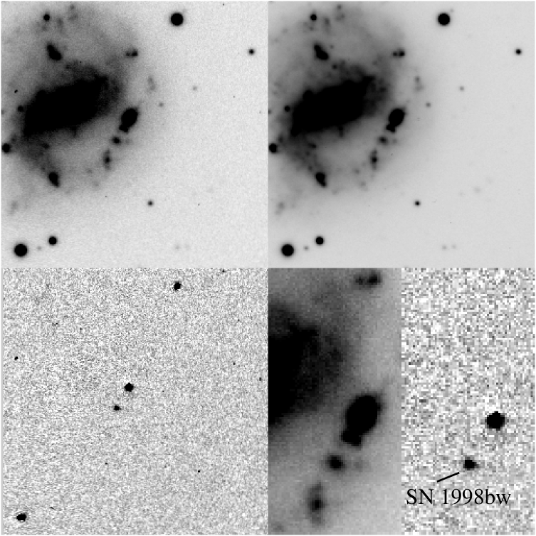
Figure 2: Illustration of the template subtraction method. Upper left shows the supernova and its galaxy as observed with the VLT in 1999 September, 503 days past explosion. Upper right is the template image. North is up and East to the left; the field of view is about $52\arcsec\times 52\arcsec$. The subtraction is shown in the lower left. Only the supernova, as well as some residuals from stars that are saturated in the template frame, are seen. Lower right shows a blowup of the supernova region, before and after subtraction. Note how the galaxy is completely subtracted.

The instrumental magnitudes were finally converted using local standards measured by Galama et al. (1998b). This worked well for the $B$-band, where four standard stars showed a standard deviation of $\leq 0.03$ magnitudes. Most of this scatter is in fact due to the neglect of color terms, which, however, do not affect the supernova as we chose a primary standard with similar color as the SN itself. For the other bands, all Galama standards were saturated in the long exposures required at these late phases. We then established secondary, faint local standards. The magnitudes of four of these local standards are presented in Table 3, together with their angular offsets from the supernova. The standard deviations for these stars measured over all the epochs were never higher than 0.03 magnitudes. Adding this to the uncertainty reported by Galama et al. for their standards, we consider the accuracy of the secondary standards to be about 0.06 magnitudes.

Table 3: Magnitudes of Faint Local Standards

Offsets from SN	$V$	$R$	$I$
$46\arcsec$ N, $17\arcsec$ W	19.77	19.03	18.45
$50\arcsec$ N, $27\arcsec$ W	21.13	19.95	18.69
$17\arcsec$ N, $26\arcsec$ W	21.64	20.44	19.12
$30\arcsec$ S, $17\arcsec$ E	21.24	20.37	19.63

2.2 Late Upper Limits

At our last epoch of VLT observations prior to the template images, i.e., at 706 days past explosion, the supernova is not detected in the subtracted images. We have used these difference images to estimate upper limits on the supernova magnitude in the following way. We measured the fluxes in a number of apertures located next to the supernova. From these measurements we estimated the standard deviations in a 5 pixel radius aperture, corresponding to the image FWHM. This estimate was then used to acquire $3\sigma$ upper limits within the aperture. These limits are 25.1, 25.1, 25.1, and 24.7 in $B$, $V$, $R$, and $I$, respectively. This procedure is more conservative than a simple measurement of the statistics in the region of the supernova. We also verified that a $R=25.1$ supernova would indeed have been detected by adding such a star to the original frame, and recovering the magnitude in the subtracted frame. This would thus provide conservative upper limits on the flux of the supernova at this epoch. The main assumption is that the supernova was indeed absent in the template frame. This is further elaborated below.

2.3 The Near-Infrared

Here, we present the last infrared (IR) observations of SN~1998bw of which we are aware.

SN~1998bw was observed using ISAAC on the VLT on 1999 May 1, 370 days after the explosion. The observations were obtained in Autojittermode, offsetting the telescope within a $60\arcsec$ wide box. Five frames were obtained in the $J$-band (1.11–1.39 $\mu$m), each one composed of a stack of five 30 second exposures. The total exposure time in the $J$-band was thus 750 seconds.

In the $H$-band (1.50–1.80 $\mu$m) five frames composed of five 20 seconds exposures yielded a total exposure time of 500 seconds. In addition, an infrared spectrum was obtained at this epoch, but the signal-to-noise ratio of this spectrum is low, and we will not discuss it further. Instead, we will use the two acquisition images to determine the IR contribution at these late phases.

The reductions were done using IRAF. From each image we subtracted a mean sky, constructed from combining all the other frames with suitable clipping to remove objects. Flat field corrections were applied using dome flat-fields. The images were then stacked and combined. The FWHM in the combined frames were $0\aas@@fstack{\prime\prime}4$ and $0\aas@@fstack{\prime\prime}55$ for $J$ and $H$, respectively.

For the calibration of the photometry, we used the zero points determined for this specific night at the VLT, from observations of photometric standards. To check the stability of the zero point, we also re-measured three local standard stars from the three earlier epochs obtained with NTT/SOFI (P01). The standard deviation in the standard stars on the three SOFI nights were 0.04 and 0.02 magnitudes in $J$ and $H$, respectively. The magnitudes agreed with the ISAAC measurements to better than 0.05 magnitudes, with a scatter of 0.02 mag.

In the combined frames, the SN magnitude were measured with PSF photometry using DAOPhot within IRAF. The measured magnitudes are $J=20.16$ and $H=19.54$. The aperture correction was obtained from the three local standards, with a negligible scatter. The DAOPhot measurement error was 0.03 ($J$) and 0.06 ($H$) magnitudes. The total error budget for the photometry is therefore certainly better than 0.1 magnitudes in both bands. These results should be treated with some caution, however, as we know from the optical data that PSF fitting may not be the best technique for this supernova.

3 The Last Phases with HST

3.1 STIS Observations

In order to follow the supernova to very late times, and to get a better understanding of the supernova environment, we have obtained detailed imaging at four epochs using the Space Telescope Imaging Spectrograph (STIS) onboard the HST. A log of our HST observations is given in Table 4.

Table 4: Log of HST Observations

Date	MJD	Epoch	Exp. Time	Exp. Time
(UT)		(days)	CL (s)	LP (s)
11 June 00	1707	778	1240	1185
25 June 00	1721	792	5672	—
21 Nov. 00	1869	940	4000	1319
28 Aug. 01	2150	1221	5674	—

The observations on 2000 June 25, 2000 Nov. 21, and 2001 Aug. 28 were taken as part of the Supernova Intensive Study programme (P.I. Kirshner). The data from 2000 June 11 was taken as part of the Survey of Host Galaxies of Gamma-Ray Bursts (P.I. Holland, Holland et al. 2000). The total exposure times in the 50CCD (clear, CL) aperture were 1240, 5672, 4000, and 5674 seconds on the four epochs, respectively. The 50CCD aperture has a central wavelength of 5850 Å and a width of 4410 Å.

In addition to the CL frames we also obtained some images in the F20X50LP (long pass, LP) filter at two epochs. The total exposure times were 1185 and 1319 seconds, respectively. The F28x50LP aperture has a central wavelength of 7320 Å and a width of 2720 Å.

The 2000 June 11 images were taken using a four-point STIS-CCD-BOX dithering pattern with shifts of 2.5 pixels ($=0\aas@@fstack{\prime\prime}127$) between exposures. The other images were dithered using the same pattern with shifts of 5 pixels ($=0\aas@@fstack{\prime\prime}254$).

The data were preprocessed through the standard STIS pipeline and combined using the dither (v2.0) software (Fruchter & Hook 2002) as implemented in IRAF. We selected a final output scale of $0\aas@@fstack{\prime\prime}0254$/pixel, corresponding to exactly half the original size, and set the “pixfrac” parameter to 0.6. Since there were only two images taken using the LP filter on 2000 Nov. 21 we had to increase “pixfrac” to 1.0 for these data in order to fill all pixels in the output frame. This resulted in a reduction in the image quality of this data compared to the drizzled 2000 June 11 LP image. The six drizzled images were finally reregistered onto a common system.

3.2 Photometry

The supernova is located in a complex region of the host galaxy (Fig. 1). There are several objects within a radius of $1\arcsec$ from the supernova position, and SN~1998bw itself is located on top of an extended, filamentary structure. In order to perform photometry of the supernova without contamination from the underlying structure we again used the template subtraction method to subtract the 2001 Aug. 28 CL image from each of the other CL images. An example subtraction is given in Fig. 1.

We then constructed PSFs for each subtracted CL image using DAOPhot II/AllStar (Stetson 1987; Stetson & Harris 1988) and fit these to the image of the supernova on each subtracted frame. We computed aperture corrections for each frame using several isolated stars. The PSF magnitudes were corrected to an aperture with a radius of $1\aas@@fstack{\prime\prime}108$, which Table 14.3 of the STIS Instrument Handbook suggests contains 100% of the flux from a point source. These corrections were about 0.1 magnitudes at all epochs. The instrumental magnitudes were converted to the AB system using the zero points of Gardner et al. (2000).

In order to understand any systematic errors we performed a series of artificial star tests on each CL image. We added a set of stars with known magnitudes comparable to that of the supernova to locations on each frame where the underlying structure was similar to the underlying structure of SN~1998bw. We then subtracted the template image and performed photometry on these artificial stars in exactly the same way as for the supernova. The resulting median differences between the input and recovered magnitudes of the artificial stars were always below 0.2 magnitudes. We regard this as a conservative error on the difference photometry.

No template image was taken using the LP filter. Therefore, no reliable magnitudes could be obtained in this band. For the 2000 June 11 image we estimated the supernova magnitude by pure PSF fitting on the drizzled image. The estimated magnitude is LP${}_{\mathrm{PSF}}=25.02\pm 0.07$. Note that there was an error in the LP aperture corrections used by Fynbo et al. (2000). That paper also contains some color information on the surrounding objects, although a correction of -0.51 mag should be added to all those LP magnitudes. The PSF magnitude for the supernova will clearly also include some of the light from the underlying background, which will result in overestimating the flux from the supernova. As mentioned above, the 2000 Nov. 21 LP frame is less useful. Visual inspection of that frame does show the supernova, just as in the CL frame from the same epoch, but we were not able to perform a reliable PSF estimate of its magnitude, since the remaining PSF residuals were always large. Therefore, only the CL magnitudes will be discussed below.

4 Results

4.1 The Optical Light Curve from the Ground

The results of the ground based photometry are presented in Table 2, and shown in Fig. 3.

Figure 3: Ground-based $B$, $V$, $R$, and $I$ photometry of SN~1998bw as obtained with the template subtraction method. The filter band light curves have been offset as indicated for clarity.

The light curves presented in Fig. 3 are all very smooth, with the exponential decay continuing all the way to the very last data points, some 540 days past explosion. The $R$ and $I$ curves, for example, are perfectly well fit by a linear decline of 1.5–1.6 magnitudes per 100 days. This is in contrast to the results published in S00 and P01, where the very late light curve appeared to flatten out. We interpret the difference as due to the complex background of SN~1998bw, and regard the new magnitudes achieved with template subtraction as more accurate. Having seen the very complex environment of the supernova in HST detail this may not be surprising. In fact, the total magnitude of the complex region surrounding the supernova amounts to $m_{\mathrm{V}}\sim 21$. In measuring supernovae some 2 magnitudes fainter than the background, even small errors in the PSF fitting will amount to substantial errors in the supernova magnitudes, an effect that will mimic a flattening of the late light curve. Core-collapse supernovae are known to explode in regions of star formation, and it is not unlikely that photometry of other supernovae at very late phases is hampered by similar effects (see Clocchiatti et al. 2001 for a similar discussion).

To investigate the total light emitted should try to build a bolometric light curve. We begin by constructing the $L_{BVRI}$ light curve, containing the optical emission from 4400 to 7900 Å. We have done this in the following way.

All magnitudes were converted to a monochromatic flux using the conversions in Bessell (1979). To add the missing $B$-magnitudes, a linear fit to these magnitudes was used, where the day 141 magnitude from McKenzie & Schaefer (1999) was included to constrain the early evolution. The light curve slope in the $B$-band is then the same as in the other bands. The fluxes were corrected for an extinction of $E(B-V)$=0.06 mag (Schlegel et al. 1998; P01), and then the monochromatic fluxes were simply integrated from 4400 to 7900 Å. Finally we adopted a distance of 35 Mpc to convert to luminosity ($z=0.0085$, $H_{0}=73$ km s^-1 Mpc^-1). To the resulting $L_{BVRI}$ points we will add a constant IR contribution in Sect. 4.4 to arrive at the light curve presented in Fig. 4.

Figure 4: The OIR light curve of SN~1998bw. The luminosities have been derived using the techniques described in the text. A constant IR contribution of 42%, as observed on day 370, has been added to all phases. The data up to 700 days are from ground based observations, and the later epochs are obtained with HST. The two error bars plotted indicate the uncertainty from 0.3 mag errors in the photometry. The arrows represent $3\sigma$ upper limits.

The slope of the late time decline is well fit by a linear decay in absolute magnitudes by 1.55 magnitudes per 100 days from 140 to 538 days past explosion. This is certainly faster than the decay rate of the radioactive $\@element[56]{\mathrm{Co}}$ powering the supernova at this phase, again showing that most of the gamma-rays are slipping out of the ejecta at late phases (S00). We discuss this further in Sect. 5.

4.2 HST Observations

The photometry from the HST observations is presented in Table 5. The CL magnitudes are the AB magnitudes measured by DAOPHOT on the template subtracted frames and with aperture corrections applied (CL_Sub). The errors are simply the formal errors from DAOPhot added to the standard deviations in the aperture corrections. This may be a bit optimistic, and from the artificial star test presented in Sect. 3.2 we regard an additional systematic error of 0.2 magnitudes as a more reliable estimate of the errors. In Table 5 we have also included the magnitudes measured on the drizzled frames using DAOPhot PSF-fitting (CL_PSF). These clearly overestimate the flux of the supernova by including also light from the underlying structure, emphasizing the need of template subtraction even at the resolution achieved by HST.

Table 5: HST/STIS photometry of SN 1998bw.

Date	CLPSF	CLSub
11 June 00	$25.33\pm 0.06$	$25.90\pm 0.05$
25 June 00	$25.45\pm 0.05$	$26.03\pm 0.04$
21 Nov. 00	$26.04\pm 0.10$	$26.88\pm 0.06$
28 Aug. 01	$\sim 27.4\pm 0.1$	$\ga 28.5$

AB-magnitudes from the STIS observations. The CLEAR-filter magnitudes obtained by template subtraction are labelled CL_Sub. The magnitudes estimated directly from PSF-fitting (CL_PSF) clearly overestimate the supernova luminosity.

The very first result to note is, of course, the clear detection of the supernova in the subtracted frames (Fig. 1). Fynbo et al. (2000) used VLT imaging (S00) to establish the position of the supernova in their STIS images. Based on this, they suggested that SN~1998bw was identical to the object positioned close to the middle of this messy region. Our analysis has demonstrated that this object is indeed fading. This strongly reinforces the supernova identification and allows us to follow the supernova to very late phases.

Secondly, from the magnitudes in Table 5, and from Fig. 3, we note that the supernova light curve seems to be levelling out at the very late phases. The reason for this will be discussed in Sect. 5.

In order to test if the supernova was still present in the 2001 Aug. 28 CL image we used DaoPhot II/AllStar to fit a PSF to the light at the location of SN~1998bw. Since there was no template to subtract from this image, the PSF fit will be strongly biased by the underlying light at the location of the supernova. The aperture-corrected PSF magnitude is CL${}_{\mathrm{PSF}}=27.4\pm 0.1$. However, an examination of the residuals after subtracting the PSF for the supernova suggests that the flux from the supernova is contaminated by light from the underlying structure and by the object $0\aas@@fstack{\prime\prime}056$ south of the supernova. To estimate an upper limit we again performed an artificial star test by injecting stars of different magnitudes onto regions of similar background as the supernova position. For input magnitudes fainter than $\sim 29-30$, we found that the recovered PSF magnitudes were always close to 27.4, as measured for the supernova position. Using the standard deviation of the recovered magnitudes as a one sigma error, we find the $3\sigma$ upper limit of about 28.5 for the supernova. This can be regarded as an upper limit on the emission from the supernova in the CL band 1221 days past explosion. This suggests that the supernova continued to fade well into 2001 at a rate similar to that observed between June and November 2000.

4.3 Combining the datasets

In measuring the ground based photometry, we made the implicit assumption that the supernova had completely disappeared in our last VLT template images. From the HST results we now know that the supernova was still there at this phase, although very faint. In fact, at a magnitude of $\sim 26.7$ on day 907 the supernova will not affect any of the ground based measurements by more than 0.05 magnitudes. We will make no correction for this effect.

However, our late VLT upper limit may indeed be significantly affected, by up to 0.25 magnitudes. We have taken this into account in the combined upper limit on the luminosity presented in Fig. 4.

Better spatial resolution clearly allows more accurate subtractions and thus photometry. It is clear, however, that even with HST there may be unresolved substructures contributing to the PSF. At 35 Mpc each drizzled pixel corresponds to 4.3 parsecs on the sky. In Table 5 we have included the magnitudes obtained with PSF-fitting on the drizzled frames, and it is clear that such an approach overestimates the flux in the supernova. The effect increases at later phases and would again make the light curve flatten. This effect should, however, be correctly accounted for using the template subtraction. We therefore believe that the flattening of the late light curve as observed by HST is a robust result.

There is again the issue of contamination from remaining supernova flux in the HST template frame. Our estimate of the upper limit on the supernova CL magnitude in the 2001 August frame is $M^{\mathrm{AB}}_{\mathrm{CL}}\ga 28.5$. If the supernova was really at this magnitude in the template frame, the supernova would be brighter than estimated in June and November 2000. The effect could amount to 0.1 magnitudes in June and some 0.2–0.3 magnitudes in November. This is an uncertainty we can not overcome without further deep and very late imaging. Here we only note that such a contamination will not dramatically affect the late light curve slope. It would only flatten the late light curve between 778 and 940 days from a slope of 0.6 magnitudes per 100 days to 0.5 magnitudes per 100 days.

It is also non-trivial to compare directly the photometry obtained in the very broad CL filter with the ground based data. Established conversions as those presented in Rejkuba et al. (2000) are based on stars, and the late supernova spectrum differs from any stellar spectrum. Simply integrating a flat spectrum over the FWHM is a crude approach for such a wide filter. Nakamura et al. (2001a) assumed that ($M_{\mathrm{AB}}=$) $M_{\mathrm{V}}=M_{\mathrm{bol}}$ to put the photometry of Fynbo et al. (2000) onto their “bolometric” light curve. Such an estimate differs by a factor 1.8 from the simple integration.

The correct approach would of course be to use the supernova spectra obtained at the same epochs for the corrections, but no such spectra are available. The latest spectrum from S00 is from 504 days past explosion. However, this spectrum is rather noisy and may be contaminated by the nearby objects revealed by HST.

We have taken the following approach to compare the different observations. From the broad band VLT photometry we do get a gross spectral energy distribution (SED) for the epochs up to 540 days past explosion. This distribution is seen to evolve fairly slowly with time and should not be influenced by the nearby objects. At all epochs, most of the energy (${\nu}F_{\nu}$) emerges in the $R$-band. From the late-time spectroscopy in S00 we know that this is mainly due to the strong [O i] $\lambda\lambda$ 6300,6364 lines. We will assume that the same gross spectral distribution is appropriate at the late HST phases, with a fairly small contribution from the $U$-band (P01) and a continuation of the SED into the IR as observed on day 370.

We then used SYNPHOT to scale this SED to give the measured count rates for the CL filter function. The scaled SED can then be integrated, after a correction for extinction (Fitzpatrick 1999), and converted to luminosity as above. We noted that the count rate in the CL filter does not depend much on the assumed SED outside the $L_{BVRI}$ range. Assuming no flux outside 4000–8000 Å decreased the measured counts by only $\sim 14$%, as both the SED and the CL filter curve peak in the middle of this interval. To avoid assumptions on the non-observed SED regimes we therefore integrated the SED only over the 4000–8000 Å range, to make it directly comparable to the ground based data.

4.4 The OIR Light Curve

An uncertainty in the bolometric light curve of P01 was the contribution of the IR emission. They assumed that the fraction of the $UVOIR$ emission escaping in the IR was the same at late times as it was on day 65, the last day covered by their IR observations. Then the IR ($JHK$) contained $\sim 35$% of the supernova emission, and this constant fraction was added to the optical light curve at all later phases (P01).

It is true that for the well observed SN~1987A, the fraction of the energy emerging from the supernova in the $V$, $R$, and $I$ bands ($L_{VRI}$) was virtually constant ($\sim 40$%) up to 400 days after the plateau phase (Schmidt et al. 1993). However, the physics of a rapidly expanding, hydrogen-free ejecta will differ from the case of SN~1987A. As the radioactive heating decreases and the ejecta expand, the gas will cool down and a larger fraction of the emission may therefore be pushed into the IR. The assumption of constant IR contribution at late phases should therefore be checked.

To estimate the contribution in the IR we followed the same procedure as outlined above for $L_{BVRI}$. The optical emission was interpolated on day 370 and integrated from $B$ to $I$. The total emission was then calculated by including also the $J$ and $H$-bands in the integral, where the conversions to flux from Wilson et al. (1972) were used. The result is that at this epoch 42% of the emission emerges in the near-IR. The same exercise for the data of day 65 gives a fraction of 31% (comparing $L_{BVRI}$ to $L_{BVRIJH}$). At all epochs, most of the energy emerges in the $R$-band.

It is thus clear that the importance of the near-IR has increased with time, although the effect is not dramatic.

To complete our OIR (optical-infrared) light curve we have simply added the IR fraction observed at day 370 to all the dates on the light curve presented in Fig. 3. This assumes that the IR contribution does not evolve at the last HST phases.

5 Discussion

The final OIR light curve is admittedly and necessarily based on a number of assumptions, but we are confident that the basic features of the light curve, the steep decline followed by a late flattening, are real. In this section we will discuss a few possible interpretations for such an evolution.

We first note the steep exponential decline seen in the ground based observations. This fast decline appears to have started already about 65 days past the explosion (McKenzie & Schaefer 1999; S00), and the light curve continues to fall significantly steeper than the decay rate of $\@element[56]{\mathrm{Co}}$ up to more than 500 days past explosion. There is thus no sign for a “positron phase” in which the fully deposited kinetic energy from the positrons would dominate the light curve. Two different scenarios could account for this.

One is that the optical depth for gamma-rays, albeit decreasing, may always be large enough to dominate over the positrons. An example is shown below (Fig. 5). Alternatively, the positrons may indeed dominate at late phases, but some of the positrons are able to escape the ejecta before being thermalized.

The second characteristic to note in the very late-time light curve of SN~1998bw is the flattening of the light curve at the last phases, as observed by HST. The late-time light curves of core-collapse supernovae can be powered by several mechanisms (see e.g., Sollerman et al. 2001), as will be further discussed below.

5.1 Radioactive Powering?

The contributions from different radioactive elements to late supernova light curves were discussed by Woosley et al. (1989). Only in SN~1987A has a radioactive decay other than ($\@element[56]{\mathrm{Ni}}$$\rightarrow$)$\@element[56]{\mathrm{Co}}$$\rightarrow$$\@element[56]{\mathrm{Fe}}$ been unambiguously observed to power the late light curve. Also for this supernova, a flattening of the light curve was observed after about 800 days. The reason for this was actually two-fold. First, at these late phases the radioactive decay of the more long-lived nucleus $\@element[57]{\mathrm{Co}}$ became important. Secondly, the long recombination scale allowed energy stored at earlier epochs to contribute at later phases (Clayton et al. 1992; Fransson & Kozma 1993). This is known as the “freeze-out” effect.

For SN~1998bw, with its very high explosion energy, the discussion must also take into account that the optical depth to gamma-rays decrease very rapidly. The high explosion energy also opens the possibility for different nucleosynthesis (Nakamura et al. 2001b).

The decreasing optical depth to gamma-rays is obvious from the first part of the light curve, as mentioned above. A very simplistic model to account for this in terms of radioactive decay is presented in Fig. 5. In this model the flux from the decay of $\@element[56]{\mathrm{Co}}$ evolves as $\mathrm{e}^{-t/111.3}\times\left(1-0.965\mathrm{e}^{-\tau}\right)$, where the optical depth, $\tau={(t_{1}/t)}^{2}$, decreases due to the homologous expansion. Here, 111.3 days is the decay time of $\@element[56]{\mathrm{Co}}$ and $t_{1}$ sets the time when the optical depth to gamma-rays is unity. Furthermore, 3.5% of the energy in these decays is in the form of the kinetic energy of the positrons, which are assumed to be fully trapped. This model can reasonably well mimic the observed light curve from day 64 to day 538 for a value of $t_{1}=105$ days (Fig. 5). This means that the trapping of gamma-rays is almost complete at day 64, but that the positron contribution is not dominating until after $\sim 600$ days.

Figure 5: Using a very simple model for the radioactive powering of SN~1998bw, a reasonable fit to the data can be achieved. The model is described in the text. The powering of $\@element[56]{\mathrm{Co}}$, $\@element[57]{\mathrm{Co}}$, and $\@element[44]{\mathrm{Ti}}$ contributes at progressively later phases. The early observations marked by crosses are from P01 and shifted to a distance of 35 Mpc.

At the HST phases the light curve flattens out and can no longer be explained in terms of $\@element[56]{\mathrm{Co}}$. An interesting possibility is then a contribution from $\@element[57]{\mathrm{Co}}$, in particular since the decay rate in the HST detections seems to agree well with the decay time of $\@element[57]{\mathrm{Co}}$$\rightarrow$$\@element[57]{\mathrm{Fe}}$.

However, the decay of $\@element[57]{\mathrm{Co}}$ has no positron channel. A fairly large amount of $\@element[57]{\mathrm{Ni}}$ (which quickly decays to $\@element[57]{\mathrm{Co}}$) must therefore be synthesized in the explosion, in order to make a significant contribution in this model.

In Fig. 5 we have included a ratio of $\@element[57]{\mathrm{Ni}}$/$\@element[56]{\mathrm{Ni}}$ which is three times larger than the ratio observed in SN~1987A. The optical depth to gamma rays is also enhanced by a factor of 2.4 as compared to $\@element[56]{\mathrm{Ni}}$, to allow for the smaller gamma-ray energies involved (Woosley et al. 1989). In addition, $\@element[44]{\mathrm{Ti}}$ has also been added with a three times larger ratio. This nucleus contributes at much later phases in SN~1987A (Kozma 2000; Lundqvist et al. 2001), but can become important at relatively earlier phases in SN~1998bw as it has a significant positron channel.

Although these abundance enhancements are quite arbitrarily chosen to match the observations, we emphasize that the nucleosynthesis yields may indeed be different for very energetic and possibly asymmetric explosions. Nakamura et al. (2001b) and Maeda et al. (2001) clearly show that enhanced amounts of ⁴⁴Ti may be expelled in such circumstances. We therefore note the possibility that the late light curve of SN~1998bw can be explained in terms of radioactivity, if the abundances of the radioactive isotopes are enhanced compared to the case of SN~1987A.

Although the above model is clearly too simplistic to give accurate results, it can be used to estimate the amount of $\@element[56]{\mathrm{Ni}}$ needed to power the supernova at a distance of 35 Mpc. With the radioactive luminosities properly included (Kozma & Fransson 1998) we have used a nickel mass of $0.3\leavevmode\nobreak\ {\leavevmode\nobreak\ \rm M}_{\odot}$ to power the light curve in Fig. 5.

This is close to the lower limit obtained by S00. This is indeed a lower limit, as the simple model forces the gamma-rays to be almost fully trapped at day 65, at the start of the rapid decline. The models presented in S00, with a complete calculation of the gamma-deposition for real explosion models, trapped 6–10% of the gamma-ray energy at 400 days, while the toy model presented here traps $\sim 7$% at this epoch. Although detailed calculations are needed to accurately determine the nickel mass, it is clear that the estimates will be lower than in S00 simply because some of the light attributed to the supernova in that analysis was due to the complex background.

The above estimate is, however, not very far from the 0.4 ${\leavevmode\nobreak\ \rm M}_{\odot}$ required to power the peak of the light curve in the refined models of Nakamura et al. (2001a), especially when the different distance estimates are taken into account.

We note that a scenario where the steep light curve decline is instead due to positron escape will clearly require much higher nickel masses to account for the observed luminosity. In such a scenario the late time contribution of $\@element[57]{\mathrm{Co}}$ is less likely, because with no positron channel an unrealistically high abundance of this isotope would be required.

5.2 Other Powering Mechanisms?

It must be clarified that apart from radioactive heating, several other mechanisms could power the late light curve. None of the usual suspects can really be ruled out based on the sparse observational constraints we have at the latest phases.

Interaction with circumstellar material (CSM) is not uncommon in core-collapse supernovae (e.g., Leibundgut 1994). In the context of SN~1998bw, Tan et al. (2001) proposed an association of GRB~980425 based on a model with a high pre-supernova mass loss of $\sim$few $\times 10^{-4}$ ${\leavevmode\nobreak\ \rm M}_{\odot}$ yr^-1. Weiler et al. (2001) also argued for a CSM from radio monitoring of the supernova. However, the very fast wind expected from a WR progenitor can give a rather modest density even with a high mass loss rate, and the interaction need not give rise to optical emission. We note that as long as the supernova was spectroscopically monitored, no spectral signatures from CSM interaction were ever detected in SN~1998bw (S00). Although absence of evidence is not evidence of absence, this may constrain the most massive progenitor models.

If SN~1998bw formed a black hole which accretes matter, this could in principle show up in the late light curve (Fynbo et al. 2000). We note that the luminosity at late phases is close to the Eddington luminosity, which would require very high efficiency. Moreover, an accretion scenario should provide a power-law decay rate (Balberg et al. 2000) , which is not observed. Black hole powering is mainly expected to be seen for supernovae with very little radioactive material, because the radioactive heating will otherwise outshine the accretion luminosity. This is quite the opposite of SN~1998bw.

Another scenario for late-time emission is a light echo, as observed in SN~1998bu (Cappellaro et al. 2001). Again, we have little information available to exclude such a possibility. We can only note that the supernova appears fairly red in the day 778 data (LP versus CL), while a light echo should reflect an early blue phase.

Finally, the late light curve might also be boosted by a freeze-out effect. As mentioned above, this was observed in SN~1987A and contributed to the light curve tail powered by $\@element[57]{\mathrm{Co}}$, as illustrated in Fig. 1 of Fransson & Kozma (1993). Most of the freeze-out in SN~1987A took place in the extended hydrogen envelope, which is absent in SN~1998bw. On the other hand, the faster expansion of SN 1998bw favors a freeze-out scenario. If freeze-out was indeed important at these phases, smaller yields of the long-lived nuclei would be required to power the light curve. Detailed time-dependent modeling is needed to quantify this effect.

6 Summary

We have presented new and updated photometry of the famous GRB supernova SN~1998bw. Using the template subtraction technique we have revised the late-time light curve and shown that the fast decline rate continues to more than 500 days past explosion. This highlights the observational problem of accurate photometry in complex regions, where core-collapse supernovae are known to reside. We note that no sign of a fully trapped $\@element[56]{\mathrm{Co}}$ positron phase is observed. A simple radioactive model with $\sim 0.3$ ${\leavevmode\nobreak\ \rm M}_{\odot}$ of ejected $\@element[56]{\mathrm{Ni}}$ can fit the data, and can be regarded as a lower limit to the amount of ejected nickel in SN~1998bw. Our very late HST observations allowed us to follow the supernova to $\sim 1000$ days, and to detect a late flattening of the light curve. One of the possible scenarios to explain this is the contribution of radioactive isotopes with longer life times. This could require different nucleosynthesis for the very energetic SN~1998bw than for SN~1987A.