Developing Diagnostics of Molecular Clouds
Using Numerical MHD Simulations

Abstract

An important aspect of astrophysical MHD turbulence research is developing diagnostics to connect simulations with the observable universe. Turbulent systems are by definition structurally complex in all fluid variables (density, velocity, and magnetic field), such that they must be described statistically. By developing and applying diagnostic tools to simulation data, it is possible to interpret empirical laws for the statistical properties of observed systems in terms of fundamental dynamical processes, and to identify and calibrate robust probes of physical parameters that cannot be measured directly. Using several different examples, I describe how structural diagnostic analyses have already yielded significant insights into the nature of turbulent molecular clouds. I review results from several different groups, and discuss directions for future diagnostics to enhance our understanding of cloud structure and constrain models of the evolutionary course that governs star formation.

1 Introduction

As the number, range, and depth of the papers in this volume witnesses, recent progress in modeling and understanding astrophysical MHD turbulence is impressive. Even with the intensive research of several groups over the past few years, however, many aspects of the fundamental turbulence phenomenon are not yet wholly understood – which makes for continuing excitement in this emerging discipline. In using the results of MHD simulations to interpret the dynamics of the interstellar medium, the technical challenges involved in numerically modeling and characterizing turbulence are compounded by astrophysical uncertainties in posing the numerical problem to be solved. For molecular clouds, open astrophysical questions include:

• What is the source (original, and potentially, maintaining) of turbulence?

• What is the mean magnetic field strength, and variation of mass-to-flux ratio, in molecular clouds?

• What is the range of sizes and masses of molecular clouds in the Milky Way and other spiral galaxies?

• How are clouds formed? how long do they live? how are they destroyed?

From the point of view of defining an idealized problem for an MHD simulation, these astrophysical questions translate to uncertainties in the input spectral form (in space and time) of the turbulent driving, the value and variation of the plasma $\beta$ parameter, the importance of self-gravity, and the initial and boundary conditions for the simulation.

The complexity of the turbulence phenomenon demands detail and variety in the analytical methods used to characterize its structure. For application to understanding astronomical systems – where the physical inputs are uncertain, and only projected distributions are available – the eventual aim is to develop a set of simple, robust diagnostics of MHD turbulence that have direct connections to observable quantities. Potentially, there are many different avenues for this sort of analysis, and extensive exploration is required to determine what directions are most productive. Because large-scale numerical simulations of turbulence under interstellar conditions are only now becoming computationally practical, the present tasks include first the “forward” process of characterizing MHD turbulence obtained from new simulations with a range of parameter values, and then using these results to select and calibrate diagnostics for the “reverse” process of discriminating systemic parameters from observables.

As examples of the process of developing diagnostics of molecular clouds’ internal structure, kinematics, and magnetization from turbulent MHD simulations, my discussion here will focus on recent work analyzing and interpreting density and column density statistics (§2), properties and definitions of clumps (§3), linewidth-size relations (§4), and statistics of polarization maps (§5). I will update previous work (see also sto98 , ost99 , ost01 , gam01 ), present several new results, and make connections to the conclusions of other groups. Chapters in the same volume covering topics most directly related to those addressed here include those by Crutcher, Heiles, & Troland; Nordlund & Padoan; MacLow; Cho, Lazarian & Vishniac; and Zweibel, Heitsch, & Fan.

2 Density and Column Density Statistics

In general, a turbulent velocity field leads to production of significant local density variations in a compressible medium (i.e. a medium with Mach number ${\cal M}\equiv v_{\rm rms}/c_{\rm s}\gg 1$, where $v_{\rm rms}$ is the turbulent velocity dispersion and $c_{s}$ the sound speed). This is true regardless of the magnetic field strength, because in the case of a weak magnetic field ($v_{\rm A}\equiv B_{0}/\sqrt{4\pi\bar{\rho}}\sim c_{s}\ll v_{\rm rms}$, where $\vec{B}_{0}$ is the mean magnetic field and $\bar{\rho}$ is the mean density), magnetic pressure forces are weak compared to ram pressure, and in the case of strong magnetic fields ($v_{\rm A}\sim v_{\rm rms}$), compression is unhindered along the mean field direction (and indeed enhanced by forces associated with gradients in $B_{\perp}^{2}$, where $\vec{B}_{\perp}$ is the component perpendicular to $\vec{B}_{0}$).

If compression and rarefaction events are spatially and temporally independent, then for the case of an isothermal equation of state (approximately true under molecular cloud conditions), the resultant one-point density distribution function (often referred to as a “PDF” – probability distribution function) is expected to obey a lognormal form (pas98 , nor99 ). If $1+\delta_{i}$ is the enhancement/decrement factor for density in the $i^{th}$ compression/rarefaction event affecting a given fluid element, then the density after $N$ events will be

$$\rho=\bar{\rho}\mbox{{P}}_{i=1}^{N}(1+\delta_{i})$$ (1)

so that the logarithm of the density,

$$\log(\rho/\bar{\rho})=\mbox{{S}}_{i=1}^{N}\log(1+\delta_{i}),$$ (2)

will be the sum of independent random variables; by the Central Limit Theorem, this implies that $\log(\rho/\bar{\rho})$ should obey a Gaussian distribution.

The results of numerical simulations (vaz94 ,pad97 , pas98 ,ost99 ,ost01 ) indeed bear out the expectation that a log-normal form for the volume density PDF prevails (at least away from the tails) under isothermal conditions. This result holds both for forced and decaying turbulence, and for simulations with varying mean magnetic fields. Figure 1 shows an example of the distributions of fractional volume and mass as a function of volume density for four forced-turbulence MHD simulations with ${\cal M}=5$ (see sto98 for details on the models), with comparisons to the lognormal functions with the same mean and dispersion.

Figure 1: Distributions of fractional volume (solid curves) and fractional mass (dashed curves) as a function of density for Mach-5 forced turbulence simulations with varying mean magnetic field strength characterized by $\beta\equiv c_{\rm s}^{2}/v_{\rm A}^{2}$, for $v_{\rm A}=B_{0}/\sqrt{4\pi\bar{\rho}}$. Dotted curves show lognormal distributions for comparison. Each panel is also labeled with the mass- and volume-weighted mean compression magnitudes.

As the example in Fig. 1 shows, the average mass compression factor is relatively insensitive to the mean magnetic field strength. Although the minimum value of the mass-weighted mean $\langle\log(\rho/\bar{\rho})\rangle_{M}$ increases (logarithmically) with the fast-magnetosonic Mach number ${\cal M}_{\rm F}\equiv v_{\rm rms}/(c_{\rm s}^{2}+v_{\rm A}^{2})^{1/2}$, the scatter from “cosmic variance” is large enough that there does not appear to be a unique relation between ${\cal M}_{\rm F}$ (or ${\cal M}$; cf. pad97 , nor99 ) and $\langle\log(\rho/\bar{\rho})\rangle$ ost01 . Typical values of the mean compression factor for matter in the simulations, $\langle\rho/\bar{\rho}\rangle_{M}$, range over $3$–$6$ for ${\cal M}=5-9$, consistent with the compression factor needed to excite the CO molecule – rendering molecular clouds observable – when the volume-weighted density is only $n\sim 100\,{\rm cm}^{-3}$ (e.g. sco87 ).

More directly observable than the distribution of volume densities in a cloud is its distribution of column densities, corresponding to line-of-sight integrations of density, $\Sigma\equiv\int\rho\mathrm{d}s$. Heuristically, one might expect the column density at any projected position to be determined by a series of independent (in space and time) compressions and rarefactions, similarly to the process of events described in (1). The difference for column density is that each event affects only a fraction $f_{i}<1$ of the line of sight, so that the column density is given by

$$\log(\Sigma/\bar{\Sigma})=\mbox{{S}}_{i}\log(1+f_{i}\delta_{i})$$ (3)

instead of (2). The factor $f_{i}$ may be thought of as the ratio of the correlation length of a given compression/rarefaction event to the overall linear scale of the cloud along the line of sight. If the individual enhancement/decrement factors are independent random variables, then the resultant column density PDF should take on a log-normal form. Because each $1+f_{i}\delta_{i}$ is closer to unity than $1+\delta_{i}$, however, the mean and dispersion of $\log(\Sigma/\bar{\Sigma})$ are expected to be smaller than the corresponding quantities for $\log(\rho/\bar{\rho})$. These expectations are indeed borne out by analyses of column densities in simulations, as shown by ost01 ; distributions show a lognormal form (see also Fig. 2), and typical values of the mass-weighted mean column density are $\langle\Sigma/\bar{\Sigma}\rangle_{M}=1.1-1.4$ for ${\cal M}=5-9$.

Figure 2: Distributions of fractional area (histograms) as a function of column density for Mach-7 decaying turbulence, for two different projection directions, from $\beta=0.01$ simulation (see ost01 for details). Solid curves show the corresponding lognormal distribution fits; dashed lines indicate exponential fits on high-column side, with slopes -1.1 and -1 for the $\hat{x}$ and $\hat{z}$ projections.

From (3), note that if the factors $f_{i}$ are small (corresponding to having the dominant correlation length small compared to the size of the numerical box/physical cloud), then $\delta\Sigma/\bar{\Sigma}\equiv\Sigma/\bar{\Sigma}-1\approx\mbox{{S}}_{i}f_{i}\delta_{i}$, implying a Gaussian distribution for $\delta\Sigma/\bar{\Sigma}$ if the terms $f_{i}\delta_{i}$ are independent random variables. Numerical evidence on how column PDFs transition from Gaussian to lognormal form as $f_{i}$ increases is presented in vaz01 .

Preliminary comparisons between observed PDFs of column density in filamentary molecular clouds – obtained from stellar extinction data alv98 – and simulated PDFs from turbulence models are very encouraging ost01 . The data are consistent with lognormal distributions, with comparable width to those from simulations having turbulent Mach numbers and power spectra comparable to those in observed clouds. It remains to be seen how much more specific information about a cloud can be learned from its column density. Although there were earlier some hopes that column density PDFs could help distinguish the mean magnetic field strength in clouds pad99 , models with matched Mach numbers “observed” from varying directions do not show strong or consistent correlations of the mean column density contrast with the value of $\beta\equiv c_{\rm s}^{2}(B_{0}^{2}/4\pi\bar{\rho})^{-1}$ ost01 . In spite of this insensitivity to the mean magnetic field strength, one might still hope to constrain the distribution of volume densities from the distribution of a cloud’s column densities. The mathematical degeneracy between $\delta_{i}$ (the volume compression/rarefaction increment) and $f_{i}$ (the spatial coherence length of an event) evident in (3) indicates that there is no simple inversion method. Methods that combine the column PDF with the spatial (two-point) correlation function in column density maps (reflecting $f_{i}$, or more generally, the shape of the density power spectrum) may however be able to lift this degeneracy; this represents an important direction for future study.

Because the population of the tails of the density and column density PDFs may be more affected by intermittency than the population near the peak, and because the equation of state may depart from isothermality in more overdense, optically thick regions (cf. sca98 ,nor99 ) observational departures from log-normality are more likely to occur there. Simulations (even with a uniform, isothermal equation of state) show a variety of behaviour in the tail distributions, although PDFs that are lognormal over more than three orders of magnitude are common from isothermal decaying-turbulence simulations. Fig. 2 shows, for example, that for column densities less than $\Sigma/\bar{\Sigma}=4$ (corresponding to some 98% of the projected area of the particular simulation), a lognormal function is an excellent approximation.

Over a limited range of column densities above the mean, lognormal PDFs can typically be fit by an exponential function as well (i.e. $\log[dA/d\Sigma]=C_{1}+C_{2}\Sigma/\bar{\Sigma}$ for $C_{1}$ and $C_{2}$ constants). Fig. 2 shows examples of local fits of this kind with slopes $C_{2}=-1.1,-1$. Similarities between this local exponential form in simulations and in molecular-line observations bli97 , with emphasis on potential dependences of the slope on the largest density correlation scale, have been investigated by bur01 (see also ost01 for related discussion of resolution effects). It is not yet clear whether there is inherent physical significance in the local exponential form, or whether it is primarily a convenient mathematical approximation to a lognormal on the high-column-density side of the distribution where most of the observable matter is found.

3 Clumps in Turbulent Clouds

A longstanding unsolved problem in astrophysics is what determines the stellar initial mass function (IMF). Many different physical processes could potentially affect the IMF; an abbreviated list includes: (i) turbulent stresses in a large-scale cloud producing non-self-gravitating clumps with a range of masses/sizes, (ii) self-gravity in inhomogeneous clumps/cores leading to sub-fragmentation of collapsing condensations, (iii) dynamical instabilities in massive disks – formed by the initial collapse of rotating cores – fragmenting them into binary or multiple star/disk systems, (iv) outward momentum flux from stellar radiation and/or MHD winds truncating accretion onto forming stars from the outer parts of their parent cores. The relative importance to the final IMF of each of these (and other) processes remains to be determined, and major technical challenges are involved in attacking any of these questions via direction numerical simulations. The large range of scales (nine orders of magnitude!) involved in going from a cloud to a star points to the need for adaptive mesh refinement (AMR) schemes in order to follow even a portion of the overall process.

For the present, we can begin by assessing the clumpy structure produced by turbulence and self-gravity at moderate scales in uniform-grid MHD simulations of GMCs. This clumpy structure can be characterized in many ways, and applying varying methods is valuable for understanding and illustrating different aspects of the formal dynamical problem, as well as for interpreting observations.

Figure 3: Number of clumps as a function of mass for two different clump identification algorithms. Lower panel shows results of excluding clumps that lie within larger clumps; upper panel shows results of counting clumps at any given spatial scale regardless of whether they lie within a larger concentration.

One class of non-hierarchical structure-analysis methods is similar to the CLUMPFIND algorithm introduced by wil94 . In this method (see gam01 for details), one chooses a threshold volume density $\rho_{\rm th}$ (or column density $\Sigma_{\rm th}$), identifies the set of local maxima in the data cube (potentially first smoothing the data to reduce pixel noise), and then defines clumps by assigning matter at $\rho>\rho_{\rm th}$ to the nearest local maximum. The shape of a clump can be quantified by computing the ratios of principal axes in its moment of inertia tensor, and the importance of self-gravity in binding a condensation can be described, e.g., by computing the ratio of gravitational energy to the (weighted) sum of kinetic, thermal, and magnetic energies.

A full discussion of the results of applying this clump-finding method to a set of decaying-turbulence (with initial ${\cal M}=14$), self-gravitating MHD simulations is given in gam01 . Results from this analysis (taking $\rho_{\rm th}/\bar{\rho}=10$) include:

• At any time, only the high-mass wing of the clump distribution is self-gravitating;

• Characterizing the spectral shape of the high-mass wing as $\mathrm{d}N/\mathrm{d}M\propto M^{-x}$, the slope $x$ is in the range 2–3, becoming shallower over time from mergers;

• The turnover in the mass spectrum is spatially well-resolved (at $\sim 8$ grid zones across) with $M_{\rm peak}/M_{\rm tot}$ of a few times $10^{-4}$;

• The minimum clump mass is typically a factor 10 below the peak value;

• Clump shapes are intrinsically triaxial, and project to having two-dimensional axis ratios $\sim 2:1$;

• The shapes of the mass functions of apparent clumps in column density maps are similar to those of true three-dimensional clumps, but shifted to larger masses by an order of magnitude.

An interesting point is that $M_{\rm peak}$, and also the minimum mass $M_{\rm min}$ of a clump for given $\rho_{\rm th}/\bar{\rho}=10$, do not vary with the value of $\beta$. Also, although the Mach number declines by a factor 4–5 over the course of the simulations, the peak and minimum masses do not change significantly. This suggests that the mass function of clumps retains a “memory” of the dynamical history of a cloud, rather than being determined solely by the cloud’s instantaneous turbulent Mach number and spectrum (as proposed in pad00 ).

The results for typical slopes of the high-mass end of the clump mass function are intriguingly similar to the value $2.35$ for the Salpeter stellar IMF, which also appears to describe the core IMF in forming clusters and00 . Similar results have also been obtained by analysis of a variety of simulations by other groups (e.g. kle01 , pnrg00 ,bal01 ). While the conclusions from these preliminary analyses are promising, many questions still remain open. It not yet clear in general how the mass scales (the peak, minimum, and maximum) depend on the input parameters ($\cal M$, as well as the spectral shape, and potentially $\beta$) and on dynamical history. Uncertainties also remain in how three-dimensional clumps relate to clumps seen in projection, and whether the latter distribution can be used to deduce the former.

Another important set of questions is how the definition of a “clump” – both the specific clump identification algorithm with its chosen set of parameters (such as $\rho_{\rm th}$), and the overall category of algorithms in which a specific method lies – affects the results. A clear categorical distinction is between non-hierarchical identification algorithms like CLUMPFIND (in which every mass element is assigned to a single clump), and hierarchical algorithms, in which a given mass element may be counted as part of many clumps, at different levels of a hierarchy. As an astronomical analogy, it is clear that for many purposes it is valuable to count galaxies whether or not they are part of larger clusters or supercluster; counting “objects” is a function of the spatial scale under consideration.

As an example of how hierarchical considerations affect the mass spectrum, consider the distributions shown in Fig. 3. For this analysis, a “clump” is any cubic region at a given spatial scale in which the density exceeds the mass-weighted mean density for the ensemble of cubes at that scale (see ost01 for further details on this “region of contrast” algorithm). For the lower panel in Fig. 3, only clumps that do not lie within other clumps are counted for the mass spectrum; for the upper panel, the spectrum counts clumps regardless of “overlap.” As should be expected, allowing for clumps-within-clumps leads to a relatively steeper mass spectrum, with a slope $\mathrm{d}N/\mathrm{d}M\propto M^{-1.9}$ in this instance. The no-overlap spectrum is $\mathrm{d}N/\mathrm{d}M\propto M^{-1.6}$. This difference between the hierarchical and non-hierarchical mass spectra is very interesting because it is reminiscent of the difference between the steep stellar IMF, and shallower observationally-determined GMC mass functions (e.g. sol87 ). Because the density condensations produced by turbulence as “initial conditions” for collapse are hierarchically nested, this difference in slopes offers intriguing support for the idea that fragmentation during gravitationally-collapsing stages may play a crucial role in defining the stellar IMF. An important question for future AMR simulations to address is when and why gravity chooses an “inner” versus “outer” mass scale for final collapsed objects.

4 Linewidth-size Relationships

The direct observables produced by spectral-line mapping of a molecular cloud are data cubes of intensity as a function of two plane-of-sky positions and the line-of-sight velocity (in radio astronomy, the intensity is described as a brightness temperature). In principal, one would like to extract the spatial distribution of velocity and emissivity from these data cubes. Because only projected data are available, and a turbulent cloud has no spatial symmetries to exploit, direct inversion is not possible. However, one may still hope to deduce statistical properties of the turbulence from the full intensity data cube. Various complex techniques to do this are under development by several groups – including Principal Component Analysis hey97 , bru01 ; the Spectral Correlation Function ros99 ,pad01 ; and Velocity Channel Analysis laz00 , laz01 . Here, I will briefly discuss a simple technique to estimate a theoretically fundamental – and observationally much-investigated – property of turbulence, the variation of linewidth with physical size scale.

Averaged over volumes with the same size in all three directions, the mean linewidth simply reflects the underlying one-dimensional velocity power spectrum, since

$$\sigma_{v}^{2}(s)=\int\int\int_{0}^{s}\mathrm{d}^{3}x\,v^{2}(\vec{x})={1\over(2\pi)^{3}}\int\int\int_{2\pi/s}^{\infty}\mathrm{d}^{3}k\,v^{2}(\vec{k}).$$ (4)

If the turbulence has a power-law spectrum, $v^{2}(\vec{k})\propto|k|^{-\alpha}$, then $\sigma_{v}(s)\propto s^{(\alpha-3)/2}$, so for e.g. Kolmogorov or Burgers spectra with $\alpha=11/3$ or $4$, $\sigma_{v}\propto$ $s^{1/3}$ or $s^{1/2}$.

In observations, however, any region of size $s^{2}$ in projection (on the plane of the sky) in general extends over a scale at least as large along the line of sight. If $s$ is small compared to the overall scale of a cloud, $L$, then the observed linewidth from a region of projected area $s^{2}$ can have contributions from $L/s\gg 1$ volume elements of size $s^{3}$ along the line of sight. If power increases with scale ($\alpha>3$), then the velocity centroids of the multiple $s^{3}$ volume elements on average differ, such that the linewidth over the area $s^{2}$ integrated over the whole line of sight will on average exceed $\sigma_{v}(s)$, reaching up to $\sigma_{v}(L)$. However, because of the statistical nature of the distribution (e.g. if it obeys Gaussian random statistics), for some projected positions the centroids of the multiple $s^{3}$ volume elements will differ very little, such that the line-of-sight integrated velocity dispersion will be close to $\sigma_{v}(s)$. From this argument, one expects that the mean linewidth would vary weakly with projected size, whereas the lower envelope of the linewidth distribution would vary more strongly with projected size, and in fact trace the underlying three-dimensional mean linewidth-size relation. Analysis of simulation data cubes indeed bears out this expectation ost01 , as shown for example in Fig. 4.

Figure 4: Linewith-size relations for projected and 3D simulated data. Distribution (squares) shows total linewidth for apparent clumps in a map vs. linear dimension of projected clump (i.e. square root of its area); dashed line shows (linear) fitted mean linewidth-size distribution for projected clump map (slope is 0.2). Solid curve shows mean linewidth-size relation for 3D volumes from the same data cube. Data set is $\beta=0.1$ model with Mach number 5 from ost01 , with threshold density $\rho/\bar{\rho}=3$.

The foregoing discussion is helpful for interpreting well-known observational aspects of molecular cloud kinematic scalings. In particular, by relation to Fig. 4, one may understand why the mean linewidth-size relation for apparent clumps observed in molecular tracers with moderate $\rho_{\rm crit}/\bar{\rho}$ is relatively flat (e.g. stu90 ,ber92 ,wil94 ) compared to the relatively steeper “Larson’s Law” ($\sigma_{v}\propto s^{1/2}$) linewidth-size relations (cf. lar81 , sol87 ) that apply to objects that are spatially “isolated” – either because $\rho_{\rm crit}/\bar{\rho}$ is large (for dense cores within clouds) or because of phase differences with their surroundings (for molecular clouds within the atomic ISM). For tracers with critical density near the (mass-weighted) mean density in a cloud, it is not unlikely for multiple structures that are separated and in relative motion along the line of sight to contribute to the linewidth at a given position on a map. For tracers with higher critical densities, the probability of chance projections of dense condensations is much lower because there are many fewer such condensations. Spectral correlation function analyses pad01 also demonstrate that simulated spectral data cubes from higher-density tracers yield more spatial variation than do data cubes from lower-density tracers, for the same reason: the spectrum at a given point in a map from a low-density tracer samples more completely along a line of sight, and is thus more representative of the mean spectrum averaged over a whole cloud – compared to the spectrum from a high-density tracer.

This discussion of linewidth-size relations in 2D and 3D also serves to illustrate the point that coherent structures in position-velocity space in general differ from coherent structures in 3D position (physical) space; detailed analyses of simulation data cubes have shown this in a number of different ways (e.g. ost01 ,pic00 ,bal01 ). As a consequence, mass functions of density condensations, or other measures of structure in the density such as its Fourier power spectrum, cannot necessarily be obtained by treating the line-of-sight velocity as a surrogate for line-of-sight position. Instead, it is necessary to use statistical approaches to diagnose structure in the physical density distribution – just as statistical approaches are required for diagnosing structure in the velocity distribution. Depending on the relative power in velocity and density fluctuations, true density structure may be best discerned by integrating intensity over velocity and then correcting for physical superposition of dense structures using information from two-point correlation functions in the column density (see laz00 for related discussion).

5 Polarization as a Magnetic Field Diagnostic

It has long been recognized that polarization studies are important for diagnosing basic properties and structure of the ISM, because they provide relatively direct access to the elusive – but dynamically important – magnetic field (e.g. hei96 ,zwe96 ). Provided that dust grains preferentially align with short axes parallel to the local direction of the magnetic field (dav51 ; see e.g. recent review of lazar00 for thorough discussion of alignment mechanisms), an ordered $\vec{B}$-field will lead to observable polarization. For grains aligned with their short axes parallel to the local magnetic field, background stars are observed in optical/near-IR wavelengths with polarization parallel to the local magnetic field, and local dust emission is observed in far-IR/sub-mm wavelengths with polarization perpendicular to the local magnetic field. If the angle of $\vec{B}$ with respect to the plane of the sky is $i$, the local contribution to polarization is $\propto\cos^{2}i$ times the difference between long- and short-axis grain crossections times the density of polarizing grains. Taking the simplest-possible assumption of a uniform ratio of polarizing-grain density to gas density (but see below), it is straightforward to create simulated polarization maps by integrating the radiative transfer equations for the Stokes parameters (mar74 ,mar75 ,lee85 ). For a medium with optical depth $\tau\ll 1$, the fractional polarization in (thermal) emission and in dust-absorbed starlight are related by $P_{\rm em}=P_{\rm abs}/\tau$ (e.g. hil88 ), so that polarization from emission is proportional to polarization from extinction divided by the column of intervening matter.

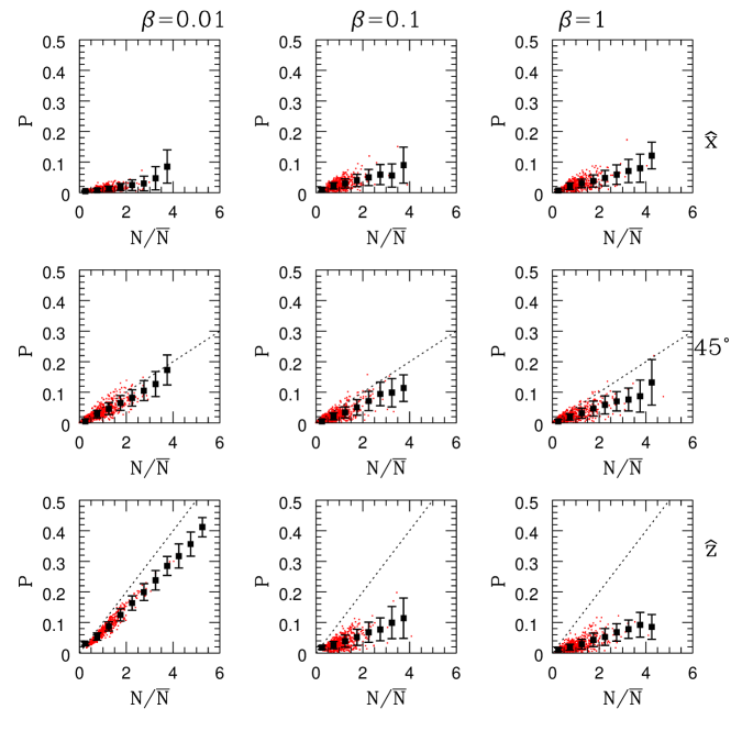
Figure 5: Distributions of simulated polarized-extinction as a function of column density, for decaying-turbulence simulations with $\cal M$=7 from ost01 . Scatter plots show $P_{\rm abs}$ for a randomly-chosen subset of positions on the projected map, for three different projection directions, and three different mean magnetic field strengths. Squares with 1-$\sigma$ error bars show the mean $P-N$ relation for the full data sets. Dotted lines show what the $P-N$ relation would be for uniform magnetic fields. $P$ is arbitrarily normalized to a value 0.1 for uniform density $N=\bar{N}$ for a projection perpendicular to $\hat{B}_{0}$

Maps and analyses of polarized extinction ost01 , and emission pgdjnr01 ,hei01 computed from MHD simulations have recently been presented by several groups. One question of interest is how the fractional polarization varies with the column $N\equiv\int n\mathrm{d}s$ of absorbing or emitting material. For a uniform magnetic field, uniform polarization efficiency of grains, but spatially-nonuniform distribution of matter, $P_{\rm abs}$ would increase linearly with $N$, while $P_{\rm em}$ would be independent of $N$. For a spatially nonuniform field, the situation is much more complicated. In this case, the increase in $P_{\rm abs}$ or $P_{\rm em}/\tau$ with $N$ would (a) in general be shallower because variations in the magnetic field direction decorrelate the direction of grains, reducing the net contribution to polarization per unit length along the line of sight, and (b) no longer follow a linear relation if the amplitude of field fluctuations is large and/or if the number of effective correlation lengths of magnetic field orientation along the line of sight varies with column density (this can yield, e.g., $P_{\rm abs}\propto N^{1/2}$ mar74 ). For weaker mean magnetic fields $B_{0}$ and a given power spectrum of fluctuations $\delta B$, the directional decorrelation in polarization occurs at a physically smaller scale than for the strong-$B_{0}$ case, so that lower polarization is expected for a given column density. These expected trends are indeed evident in distributions of $P_{\rm abs}$ vs. column density from MHD simulations, as shown for example in Fig. 5.

Interestingly, observed distributions (e.g.goo95 , arc98 ) of polarized-extinction vs. column (or $A_{V}$) in molecular clouds do not show the behavior evident in Fig. 5, which would correspond to a secular increase in $P_{\rm abs}$ up to $A_{V}$ of 30 or more (for $\bar{N}$ corresponding to a typical GMC $A_{V}\sim 7.5$ mck99 ). Instead, the observed increase of $P_{\rm abs}$ with $A_{V}$ flattens near $A_{V}$ of unity, possibly indicating that grain alignment fails in the deep interiors of clouds (e.g. laz97 ). Additional support for this idea comes from comparison of observed distributions (e.g. hen01 ) of $P_{\rm em}$ vs. intensity (proportional to $N$) in dense cores with simulated distributions; the simulations show insufficient decrease in $P_{\rm em}$ with column unless high-$A_{V}$ regions have decreased polarizing efficiency pgdjnr01 .

Potentially, one of the most important applications for polarization studies is to use the variation in polarization directions to diagnose the strength of the magnetic field cha53 . The basic physical idea behind the so-called “Chandrasekhar-Fermi” method is that weaker magnetic fields produce lower tension forces for a given displacement, so that for a given velocity field, a lower mean magnetic field strength results in larger distortions in the magnetic field direction. For the case of a single low-amplitude Alfvén wave in a uniform magnetic field with plane-of-sky component $B_{p}$, the magnetic field and velocity perturbations obey $\delta B/B_{p}=\delta v/v_{\rm A,p}$, where $v_{\rm A,p}=B_{p}(4\pi\bar{\rho})^{-1/2}$. For a wave with perturbation direction in the plane of the sky, the dispersion in polarization directions is $\delta\phi=\langle(\delta B/B_{p})^{2}\rangle^{1/2}$ if the net polarization is either parallel or perpendicular to $\vec{B}$. If there is an Alfvén wave component with perturbations along the line of sight having the same amplitude as the component with perturbations in the plane of the sky, then $\delta v/v_{\rm A,p}\equiv\langle v_{\rm los}^{2}\rangle^{1/2}/v_{\rm A,p}=\delta\phi$, so that $B_{p}$ is given by $B_{\rm CF}\equiv(4\pi\bar{\rho})^{1/2}\delta v/\delta\phi$. Thus, with measures of the mean density, the observed velocity dispersion, and the dispersion in polarization angles, the plane-of-sky field strength may in principle be estimated.

Figure 6: Plane-of-sky component of the mean magnetic field, $B_{p}$, relative to Chandrasekhar-Fermi estimate $B_{CF}$, for $\cal M$=7 (four-sided symbols) and $\cal M$=9 (five-sided symbols) decaying turbulence MHD simulations ost01 ; $\delta\phi$ is the corresponding dispersion (in degrees) of directions in the polarized-extinction map. Solid, starred, and open symbols represent $\beta=0.01,\ 0.1,\ 1.0$ models.

Since several of the idealizations described above do not hold in a real molecular cloud, it is desirable to test and/or recalibrate the Chandrasekhar-Fermi (hereafter “C-F”) relation using MHD simulations, which allow for more complex dynamical structure. Figure 6 shows an example of such a test using simulated polarized-extinction data, comparing the true mean plane-of-sky field strength with the “one-wave/equipartition” C-F estimate given above. As reported in ost01 , when the dispersion in polarization angles is sufficiently small ($\delta\phi<25^{\circ}$) – such that linear theory is adequate, a good estimate of the plane-of-sky field is $\langle B_{p}\rangle\sim 0.5B_{CF}$. Evidently, the presence of more than one wave along the line of sight reduces $\delta\phi$, so that $B_{CF}$ tends to overestimate the true $B_{p}$. For larger dispersions in polarization angle, Fig. 6 shows that the measure $0.5B_{CF}$ “calibrated” at small $\delta\phi$ may either under- or over-estimate $B_{p}$. Note that even if the mean magnetic field is strong, $\delta\phi$ can be large – and linear theory inappropriate – for system orientations in which the mean magnetic field direction lies near the line of sight. Analyses of simulated polarized-emission maps, combined with kinematic measurements hei01 , or with synthetic radiative transfer spectral maps pgdjnr01 , yield similar results for testing of the C-F formula.

Figure 7: (a) Total (rms) magnetic field strength relative to C-F estimate $B_{CF}$ vs. dispersion (in degrees) of directions in the polarized-extinction map. (b) Total (rms) Alfvén speed compared to $\sqrt{3}$ times the line-of-sight velocity dispersion. Data and symbols for (a) and (b) are as in Fig. 6.

We note that the C-F method measures only the mean plane-of-sky magnetic field $\langle B_{p}\rangle$; Figure 7(a) shows that even for small dispersion in polarization angles, there can be large variation in the total field strength compared to the “corrected” C-F estimate. In any individual cloud, the line-of-sight field can be estimated by the Zeeman effect (at least in principle; in practice this is difficult), with the two estimates combined to obtain the total three-dimensional field strength (e.g. mye91 ). Another potential caveat for observational application of the C-F method is that the principal correlation scale for the dispersion in magnetic field directions must be resolved in the plane of sky by the effective observational “beam”. For polarized extinction, this poses no difficulties because background star observations have minimal beam thickness. For polarized emission from warm cores, however, large-beam averaging of spatial fluctuations tends to reduce $\delta\phi$ relative to its value for a “pencil-beam” observation, potentially resulting in an overestimate of $B_{p}$ unless an appropriate correction factor is applied hei01 .

When variations in the polarization directions in a map are large, the fluctuations of the plane-of-sky magnetic field must be comparable to the mean value of $B_{p}$. In this case, it is not possible to distinguish from polarization studies alone whether (a) a cloud has a large mean magnetic field that is “hidden” along the line of sight (as is the case for the solid points in Fig. 6 having large $\delta\phi$), or (b) the mean magnetic field is simply weak (as is the case for the starred and open points in Fig. 6). Observed line-of-sight velocities combined with an assumption of equipartition between magnetic and kinetic energies can still yield an approximate measure of the rms magnetic field strength (see e.g. Fig. 7b) that is correct within a factor $\sim 2$, although an important caveat is that this estimate could be arbitrarily far off for cases with very strong mean magnetic fields ($v_{\rm A}\gg v_{rms}$) that happen to lie near the line of sight. Fitting formulae that interpolate between the small-$\delta\phi$ and large-$\delta\phi$ limits (with the implicit assumption that $v_{\rm A}$ along the line of sight is not very large) have been provided by hei01 .

6 Summary

To understand the intrinsic nature of MHD turbulence and the relation between the turbulence observed in astronomical systems and the turbulence simulated numerically, it is crucial to develop structural diagnostics. These diagnostics may:

• Enhance conceptual understanding of the turbulent phenomenon;

• Enable determination of astronomical systems’ properties that are either difficult to observe at all (e.g. $\vec{B}$) or only indirectly observable because of projection effects (e.g. $\vec{v}_{k}$, $\rho_{k}$);

• Provide a physical basis or interpretation for observed empirical “laws” (e.g. column density distributions, linewidth-size relations, mass functions of clouds, clumps, and stars);

• Indentify when additional physical ingredients may be needed in a computational model.

From the examples outlined in this paper, it is clear that significant advances along these lines have already been accomplished.

Conceptual and (approximate) quantitative understanding of what determines the PDFs of density and column density observed in molecular clouds have already been obtained from analyses to date (see §2). The development of lognormal statistics from Gaussian random processes under near-isothermal conditions appears to obtain robustly for a variety of conditions, with little sensitivity to the magnetic field strength. Because one-point density statistics are subject to “cosmic variance” (if low wavenumbers dominate the power spectrum, different realizations of a given power spectrum have significant variation), and because degeneracies prevent the direct inversion of column density statistics to obtain volume density statistics, there may not be a highly accurate way to determine the physically-important volume-averaged density in a cloud from more direct observables such as the observed velocity dispersion and observed distribution of extinction. Future work that combines one-point column density statistics with two-point correlation functions could potentially be valuable in constraining the spatial power spectrum of density fluctuations. Such analyses could also be useful in relating mass functions of clumps seen in projection with true three-dimensional clumps (see §3, §4).

Analysis of clumpy structure in model clouds (see §3) shows intriguing correspondence to observations: mass functions of self-gravitating structures are comparable to the Salpeter IMF, and there are significant differences between steeper (more “stellar-like”) mass functions when subcondensations are not subsumed into larger structures, and shallower (more “cloud-like”) mass functions when substructure is discounted. These findings support the concepts that clumping imposed by turbulence, as well as fragmentation during gravitational collapse, may both be important in establishing the IMF. Future work is required to determine whether there might be a relationship between Mach numbers (instantaneous and historical), the overall size and mass of a cloud, and the characteristic “peak” sizes and masses of self-gravitating condensations within a simulation. More coverage of model parameter space (allowing for different power spectra, forcing, etc.) will be important for deciding how sensitive the resulting clump mass functions may be to physical conditions.

Some of the longest-established empirical results about molecular clouds concern the correlations among physical scale and spectral linewidth, and analyses of simulations have proven valuable in interpreting how these empirical “laws” relate to the underlying properties of turbulent clouds and how they are observed (see §4). Steep (“Larson’s law”) dependence of linewidth on size probably reflects the true three-dimensional power spectrum, since the structures to which these steep laws apply are observed in tracers that render them well-separated from the background. On the other hand, the weak dependence of mean linewidth on 2D size of apparent moderate-density clumps within clouds may largely arise from projection effects – with the scale sampled by the velocity dispersion on average extending over much of the whole cloud’s depth. Both simple methods using the lower envelope of the linewidth-size distribution – and more complicated methods using detailed spectral shapes and their spatial correlations, are very promising for being able to distinguish the true three-dimensional power spectrum from molecular line data cubes.

Since magnetic fields are difficult to measure directly, there are particularly strong motivations to develop indirect diagnostics (see §5). Polarization either in absorption or emission is sensitive to the local direction of the magnetic field, and the variation in the local direction of the magnetic field is sensitive to the magnitude of the magnetic field and level of turbulence in a cloud. Thus, one might hope to combine observed measures of variation in the polarization direction with observed measures of turbulence via molecular linewidths to infer the mean magnetic field strength; this kind of indirect method was originally proposed by Chandrasekhar and Fermi. Testing the Chandrasekhar-Fermi method with simulation “data” shows that for low dispersion in the polarization angle, recalibration by a factor one-half indeed yields a good measure of the mean plane-of-sky magnetic field. When the polarization direction has large fluctuations, the Chandrasekhar-Fermi method loses accuracy, but simulations show that an assumption of magnetic/kinetic equipartition is usually correct within a factor $\sim 2$. Because underresolution tends to enhance the estimated field strength, and because high-column/high-density regions may not be efficient polarizers, there are some potential caveats in applying the Chandrasekhar-Fermi method for polarized-emission data. The promise shown by analyses to date, together with the potential to obtain large-scale maps of polarized absorption and emission in molecular clouds, marks this area as an important direction for further research.

These detailed results are exciting, and represent only a small sample of the progress that has taken place in this field to date. Perhaps the most fundamental advance, however, has been the movement to match our sophisticated concept of what a molecular cloud is – a complex structure with multiple-scale, large-amplitude, turbulent fluctuations in all fluid variables; with a commensurately sophisticated way to diagnose structure – by developing and testing analytical tools on detailed simulation data cubes that are self-consistent, time-dependent solutions of the MHD equations. Recent accomplishments have greatly advanced our field, but we are still very much in the era of discovery. Ongoing interplay between simulation, analysis, and observation will be essential for continued progress in building a comprehensive dynamical model of molecular clouds.

I am grateful to J. Stone and C. Gammie for permission to present results from collaborative work, and to the referee A. Lazarian for helpful comments. This research is supported by NASA grants NAG 53840 and NAG 59167.

References

- (1) André, P., Ward-Thompson, D., & Barsony, M. 1999, in Protostars and Planets IV, ed. V. Mannings, A. P. Boss & S. S. Russell (Tucson: University of Arizona Press), p. 59
- (2) Alves, J., Lada, C.J., Lada, E.A., Kenyon, S.J., & Phelps, R. 1998, ApJ , 506,292
- (3) Arce, H.G., Goodman, A.A., Bastien, P., Manset, N., & Sumner, M. 1998, ApJ, 499, L93
- (4) Ballesteros-Paredes, J., & Mac Low, M.-M. 2001, astro-ph/0108136
- (5) Bertoldi, F., & McKee, C.F. 1992, ApJ, 395, 140
- (6) Blitz, L., & Williams, J. P. 1997, ApJ, 488, L145
- (7) Brunt, C.M., & Heyer, M.H. 2001, ApJ, in press (astro-ph/0110155)
- (8) Burkert, A., & Mac Low, M.-M. 2001, astro-ph/0109447
- (9) Chandrasekhar, S., & Fermi, E. 1953, ApJ, 118, 113
- (10) Davis, L., & Greenstein, J. 1951, ApJ, 114, 206
- (11) Gammie, C.F., Lin, Y.-T., Stone, J.M., & Ostriker, E.C., 2001, ApJ, in preparation
- (12) Goodman, A.A., Jones, T.J., Lada, E.A., & Myers, P.C. 1995, ApJ, 448, 748
- (13) Heiles, C. 1996, in Polarimetry of the Interstellar Medium, Eds. W.G. Roberge & D.C.B. Whittet (ASP Press:San Francisco), p. 457
- (14) Heitsch, F., Zweibel, E.G., Mac Low, M.-M., Li, P., & Norman, M.L. 2001, ApJ, 561, 800
- (15) Henning, Th., Wolf, S., Launhardt, R., & Waters, R. 2001, ApJ, 561, 871
- (16) Heyer, M., & Schloerb, P. 1997, ApJ, 475, 173
- (17) Hildebrand, R.H. 1988, QJRAS, 29, 327
- (18) Klessen, R.S. 2001, ApJ, 556, 837
- (19) Larson, R. B. 1981, MNRAS, 194, 809
- (20) Lazarian, A., Goodman, A.A., & Myers, P.C. 1997, ApJ, 490, 273
- (21) Lazarian, A. 2000, in Cosmic Evolution and Galaxy Formation, Eds. J. Franco, E. Terlevich, O. Lopez-Cruz, & I. Aretxaga (ASP:San Francisco), p. 69 (astro-ph/0003314)
- (22) Lazarian, A., & Pogosyan, D. 2000, ApJ, 537, 720
- (23) Lazarian, A., Pogosyan, D., Vázquez-Semadeni, E., & Pichardo, B., 2001, ApJ, 555, 130
- (24) Lee, H.M, & Draine, B.T. 1985, ApJ, 290, 211
- (25) Martin, P.G. 1974, ApJ, 187, 461
- (26) Martin, P.G. 1975, ApJ, 202, 393
- (27) McKee, C.F. 1999, in The Physics of Star Formation and Early Stellar Evolution, Eds. C. Lada, & N.Kylafis (Dordrecht:Kluwer), p.29
- (28) Myers, P.C., & Goodman, A.A. 1991, ApJ, 373, 509
- (29) Nordlund, Å., & Padoan, P. 1999, in Interstellar Turbulence, eds. J. Franco & A. Carramiñana, (Cambridge:CUP), p 218
- (30) Ostriker, E., Gammie, C.F., & Stone, J.M. 1999, ApJ, 513, 259
- (31) Ostriker, E.C., Stone, J.M., & Gammie, C.F. 2001, ApJ, 546, 980
- (32) Padoan, P., Jones, B. T., & Nordlund, Å. P. 1997, ApJ, 474, 730
- (33) Padoan, P., & Nordlund, Å. 1999, ApJ, 526, 279
- (34) Padoan, P., & Nordlund, Å. 2000, astro-ph/0011465
- (35) Padoan, P., Rosolowsky, E.W., & Goodman, A.A. 2001, ApJ, 547, 862
- (36) Padoan, P., Goodman, A., Draine, B.T., Juvela, M., Nordlund, Å, & Rögnvaldsson, Ö.E. 2001, ApJ, 559, 1005
- (37) Pichardo, B., Vázquez-Semadeni, E., Gazol, A., Passot, T., & Ballesteros-Paredes, J. 2000, ApJ, 532, 353
- (38) Padoan, P., Nordlund, Å, Rögnvaldsson, Ö.E., & Goodman, A. 2000, astro-ph/0011229
- (39) Passot, T. & Vázquez-Semadeni, E. 1998, Phys. Rev. E, 58, 4501
- (40) Rosolowsky, E.W., Goodman, A.A., Wilner, D.J., & Williams, J.P. 1999, ApJ, 524, 887
- (41) Scalo, J, Vázquez-Semadeni, E., Chappell, D., & Passot, T., 1998, ApJ, 504, 835
- (42) Scoville, N.Z., & Sanders, D.B. 1987, in Interstellar Processes, ed. D.J. Hollenbach & H.A. Thronson, Jr. (Dordrecht:Reidel), p. 21
- (43) Solomon, P. M., Rivolo, A. R., Barrett, J., & Yahil, A. 1987, ApJ, 319, 730
- (44) Stone, J.M., Ostriker, E.C., & Gammie, C.F. 1998, ApJ, 508L, 99
- (45) Stutzki, J., & Gusten, R. 1990, ApJ, 356, 513
- (46) Vázquez-Semadeni, E., 1994, ApJ 423, 681
- (47) Vázquez-Semadeni, E., & García, N., 2001, ApJ, 557, 727
- (48) Williams, J. P., de Geus, E. J. & Blitz, L. 1994, ApJ, 428, 693
- (49) Zweibel, E.G. 1996, in Polarimetry of the Interstellar Medium, Eds. W.G. Roberge & D.C.B. Whittet (ASP Press:San Francisco), p. 486