Small Scale Structure at High Redshift: IV. Low Ionization Gas Intersecting Three Lines of Sight to Q2237+0305

Abstract

We have obtained Keck HIRES spectra of three images of the quadruply gravitationally lensed QSO 2237+0305 to study low ionization absorption systems and their differences in terms of projected velocity and column density across the lines of sight. We detect CaII absorption from our Galaxy, and a system of High Velocity Clouds from the lensing galaxy (z=0.039) with multiple CaII components in all three sightlines. Unlike the situation in our Galaxy there is no prominent CaII absorption component (with an equivalent width exceeding 60-70 mÅ) close to the velocity centroid of the lensing galaxy 2237+0305. Instead, CaII components with total equivalent widths similar to those of Galactic intermediate and high velocity clouds are spread out over several hundred kms^-1 in projection along the sightlines at impact parameters of less than one kpc through the bulge of the galaxy. A CaII absorbing thick disk like in our Galaxy does not seem to extend into the bulge region of the 2237+0305 galaxy, whereas high velocity clouds seem to be a more universal feature. We have also studied three low ionization MgII-FeII systems in detail. All three MgII systems cover all three lines of sight, suggesting that the gaseous structures giving rise to MgII complexes are larger than $\sim$ 0.5 kpc. However, in most cases it is difficult to trace individual MgII ‘cloudlets’ over distances larger than 200-300 $h_{50}^{-1}$ pc, indicating that typical sizes of the MgII cloudlets are smaller than the sizes inferred earlier for the individual clouds of high ionization gas seen in CIV absorption. We tentatively interpret the absorption pattern of the strongest MgII system in terms of an expanding bubble or galactic wind and show that the possible loci occupied by the model bubble in radius-velocity space overlap with the observed characteristics of Galactic supershells.

1 Introduction

Absorption lines in the spectra of the separate images of gravitationally lensed QSOs provide a unique opportunity to investigate the detailed structure of the interstellar gas and the intergalactic medium on scales of ten parsecs to a few tens of kpc. The ultimate goal of such observations is to study the evolution of the microstructure of the gas in galaxies and in the intergalactic medium from the epoch of formation of the first luminous objects in the universe down to the present epoch. For the past few years we have undertaken a survey of lensed QSOs with the HIRES spectrograph (Vogt et al 1994) on the Keck I telescope on Mauna Kea. The first paper in the present series (Rauch, Sargent and Barlow 1999) analyzed a low ionization absorption system at $z_{abs}=3.538$ on a scale of only 26h${}^{-1}_{50}$ parsecs. The second paper (Rauch, Sargent and Barlow 2001) investigated the structure of C IV absorbing clouds, including an estimate of the rate of input of mechanical energy, while the third paper (Rauch, Sargent, Barlow and Carswell 2001) set a limit on inhomogeneities in the “Lyman alpha forest” clouds at redshift $z\sim 3.3$.

In the present paper we turn our attention to low ionization systems which are characterized by MgII or FeII absorption lines. This gas is likely to be denser, more metal-rich, and more closely associated with galaxies than either the average Lyman $\alpha$ forest or the high ionization CIV absorption systems.

At intermediate redshifts MgII absorbers have usually been interpreted as the large gaseous halos of luminous galaxies. The sizes of entire MgII complexes are relatively well constrained: Smette et al (1995), from observations of HE1104-1805A,B, estimate lower limits of $>20h_{50}^{-1}$ kpc for the diameters of MgII systems (see also the high resolution study of the z=1.66 system in that QSO by Lopez et al 1999). Monier et al (1998) find an upper limit of $20h_{50}^{-1}$ kpc for a strong Lyman limit absorber. HIRES spectra we have obtained of the two lines of sight to UM673 A and B (to be published) show three strong MgII absorption systems. The one at z=0.426 (transverse separation between the lines of sight: $14.6h_{50}^{-1}$ kpc) shows absorption in only one of the images, whereas in the other two systems (z=0.492, sep. = $15.5h_{50}^{-1}$ kpc; z=0.564, sep. = $13.9h_{50}^{-1}$ kpc) there is MgII absorption of similar strength in both sight lines. Surveys for galaxies in the vicinity of MgII absorption systems and attempts to reconcile the total absorption cross section with the luminosity function of galaxies (Bergeron & Boissé 1991; Steidel 1995; Bowen, Blades & Pettini 1995; Churchill et al 1999) have shown that galaxies appear to be surrounded by halos of MgII gas with radii estimated to be on the order of 60-130 $h_{50}^{-1}$ kpc.

The spatial extent of individual MgII absorption components as opposed to entire MgII systems is somewhat harder to pin down. The low ionization system discussed by Rauch, Sargent and Barlow (1999) showed that SiII and CII gas cloudlets (at least at z=3.6) can be as small as a few tens of parsecs. Petitjean et al (2000) have investigated intermediate redshift MgII systems in a (spatially unresolved) HIRES spectrum of the lensed BAL APM08279+5255 and conclude from the residual intensity in the MgII doublets that the sizes of individual clouds are less than $1.5h_{50}^{-1}$ kpc. The only other independent size estimate on individual cloudlets comes from ionization calculations (e.g., Bergeron & Stasinska 1986; Steidel 1990), which, however, provide more indirect constraints. Rigby et al (2002) using such arguments, find that a subset of iron-rich MgII systems may be consistent with cloudlets as small as 10 pc in diameter.

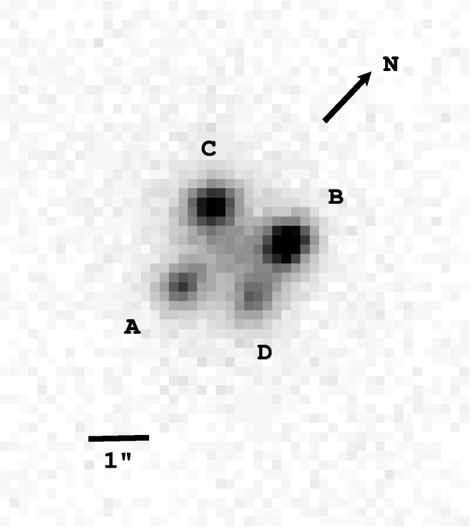
Figure 1: Keck HIRES guider camera image of Q2237+0305. The exposure time was 5 s, the picture was taken on October 21, 1998. The relative flux ratios at that date were approximately $F_{A}:F_{B}:F_{C}:F_{D}=1.0:2.1:1.7:0.7$.

In the present paper we address the question of the small scale structure of low and intermediate ionization gas in more detail. In particular, we investigate the absorption lines in the spectrum of the ”Einstein Cross” in which Q2237+0305 ($z_{em}=1.69$) is gravitationally lensed by a 15th magnitude galaxy with a redshift z = 0.0390 (Huchra et al. 1985). Subsequent work (Yee 1988) revealed that the galaxy is a barred Sb with a ring, and has a disk scale length $r_{0}=9.4"$ and an effective radius for the bulge $r_{e}=1.9"$. Q2237+0305 turned out to have four images roughly arranged in the form of a cross centered on the nucleus of the galaxy (Yee 1988; see his fig.4). The typical separation between images is less than 2”. Crane et al. (1991) obtained B = 17.96 magn. for component A, B = 17.82 magn. for B, 18.66 magn. for C and 18.98 magn. for image D. Later observations showed that the relative brightnesses of the images is subject to changes, in part due to microlensing (Irwin et al 1989). Note that the flux ratios obtained during the current observation (in the caption of Fig. 1) are very different indeed.

The original discovery spectra only showed self absorption in the Lyman alpha and C IV emission lines. Hintzen et al. (1990) searched for but failed to find Ca II H and K absorption due to the lensing galaxy in the spectra of the quasar images. However, they detected Mg II and Fe II absorption at $z_{abs}=0.5664$ and a C IV complex at $z_{abs}=1.694$ and 1.697.

In section 2 we describe the high resolution observations of the three brighter components of Q2237+0305 with HIRES. Section 3 presents the detection of CaII absorption from the Milky Way and Section 4 describes a CaII system arising in the lensing galaxy. Section 5 discusses the properties of a peculiar, strong MgII absorption and tries to give a tentative interpretation. Sections 6 and 7 briefly describe the other two low ionization systems towards Q2237+0305, and section 8 gives the conclusions.

2 Observations and data analysis

Q2237+0305 has four images roughly arranged in the form of a cross centered on the nucleus of a 15th magnitude galaxy. A picture of the lensed QSO taken off the Keck HIRES guider is shown in Fig. 1 where the four images are identified. Spectra of the three brighter images A, B and C were obtained with HIRES in October 1998. The blue cross disperser was used, giving a wavelength coverage of 3645-5204 Å which puts the C III] 1909 emission line at the red end of the range covered. We used a 0.86” slit, giving a resolution of 6.6 km s^-1. The exposures, broken into 3000 second sections, totaled 18,000 seconds on image A, 18,000 s on B and 15,000 s on C. A heliocentric correction was applied. All wavelengths quoted here are vacuum values. The individual spectra of each image were combined and scaled to the same continuum level in order to compare the details of the absorption lines. The absorption systems were fitted with the Voigt profile fitting routine VPFIT (Carswell et al 1991, 1992). Fitting components were put in until a statistically satisfying $\chi^{2}$ value was achieved. Usually this involved obtaining a reduced $\chi^{2}$ with a probability $>1\%$ to have ocurred by chance. The continuum level was treated as an additional free parameter (see paper III) to reduce systematic errors that could have crept in with the interactive continuum fitting.

The interpretation of this dataset is somewhat more challenging than usual because the QSO images closely surround (to within an arcsecond) the peaked emission from the bulge of the foreground lensing galaxy, so there is a high background level which rapidly changes in the radial direction (Fig. 1). The data show several instances of absorption lines which to the eye appear flat-bottomed and saturated while not dropping down to zero intensity in the line center. This phenomenon is most obvious in the strong absorption of the MgII complex at z=0.5656, especially in images $B$ and $C$ (see Figs. 5 and 6 and below, and the discussion in section 4.1), where there appear to be partly flat-bottomed MgII 2796 lines with a residual intensity of about 11% (in image $B$). At values of 1.35 and 1.16 the MgII doublet ratios for the strongest components in the $A$ and $C$ images, respectively, also suggest partial saturation. There are several possible explanations for this behaviour: (a) the absorbing gas cloud does not cover the continuum source of the background QSO and the troughs are partly filled in with light by-passing the absorber; (b) the absorption lines are very narrow and unresolved by the instrument; and (c) there is a foreground light source which partly fills in the absorption lines of systems arising between the foreground source and the background QSO. Possibility (a) is quite unlikely in that all of the low ionization systems are very far away from the QSO redshift. Case (b), unresolved narrow lines, may indeed by present, but the flat bottoms of the absorption lines and the fact that different lines often reach similar levels argues against it being the main effect: it would require a conspiracy between individual optical depths and velocity separation between the components to produce such a pattern. Possibility (c), pollution by the light of the bright lensing galaxy appears most likely: inspection of various strong lines in all three lines of sight shows that the residual intensities at the line bottoms correlate with the local flux of the QSO (they are weaker where the QSO is brighter, e.g., in the CIV emission line), as one would expect if the contribution of the QSO continuum light to the total spectrum increases relative to the light of the foreground galaxy. The relative contribution of galaxy and QSO continuum to the flux at a given wavelength, $F_{gal}/F^{cont}_{QSO}$, can be written in terms of the residual intensity at the bottom of an apparently saturated absorption line, $F^{res}(\lambda)$, as

$$\frac{F_{gal}(\lambda)}{F^{cont}_{QSO}(\lambda)}=\frac{F^{res}(\lambda)}{1-F^{res}(\lambda)}$$ (1)

For image $A$ the MgII 2796 line at z=0.5656 gives approximately $F_{gal}/F^{cont}_{QSO}\sim 0.08$, while the strongest CIV 1548 line at z=1.693 gives 0.04. The CIV z=1.693 line is an associated system riding almost on top of the CIV emission line and hence may be a candidate for partial continuum coverage. However, we ignore this effect here since it can only make the line less black. For image $B$ the MgII 2796 at z=0.5656 gives approximately $F_{gal}/F^{cont}_{QSO}\sim 0.11$, while the CIV 1548 line at z=1.693 gives again about 0.04. In other words the contribution of the light from the lensing galaxy to the integrated spectrum is up to about 11% near the MgII 2796 z=0.5656 system.

A naive measurement of the column densities without correcting for the light pollution by the lens would underestimate the column density for weak lines on the linear part of the curve of growth by on the order of 0 - 12% (see section 4 below), but for saturated lines they may be highly underestimated. Therefore, the column densities and measurement uncertainties in tables 1,2, 4 and 5 below (which reflect only the profile fits without correction for the residual flux from the lens) should be taken as lower limits. The exception is the $z=0.5656$ low ionization system (section 4) where many lines are obviously saturated, so a correction was attempted by simultaneously adjusting the zero level of the spectroscopic flux while fitting the absorption line profiles. The correction was possible because there were enough saturated regions to constrain the zero flux level, but it could not be applied meaningfully to the other absorption systems which appear to be mostly optically thin and do not have enough transitions available. Thus table 3 contains actual estimates of the absorption line properties.

3 CaII absorption from the Milky Way

The CaII absorption from our Galaxy can be modelled satisfactorily with a single velocity component in all three images (see the fit parameters in table 1). A pairwise comparison between any two of the three sightlines is shown in Fig. 2. The column densities and Doppler parameters are identical to within the errors, and the projected velocities along the line of sight differ by less than 2.9 $\sigma$ between the images. In other words, there is no significant difference in the appearance of the Galactic CaII systems in the three lines of sight. The mean weighted heliocentric velocity of the three sightlines is $cz=-13.9\pm 0.5$ kms^-1. The direction of the Q2237+0305 sight lines in galactic coordinates ($l^{II}$ = 71.8, $b^{II}$ = -46.1 deg) subtends an angle of $\sim 63$ deg with the heliocentric velocity vector of the local bulk flow of interstellar cloudlets within $\sim 30$ pc ($v_{\mathrm{h}elio}$ = $-28.1\pm 4.5$ kms^-1; Frisch, Grodnicki, & Welty 2002) so the projected velocity of that flow relative to the 2237+0305 line of sight would be -12.9 kms^-1. This is well consistent with the idea that the CaII observed here arises from the cluster of local interstellar gas clouds within 30 pc. The maximum angle between the three lines of sight to Q2237+0305 is about 1.8 arcsec. Thus, if the Galactic CaII absorber towards 22327+0305 resides within 30pc, our observation means that there are no significant detectable differences in that particular CaII cloudlet over transverse separations smaller than 54 astronomical units.

4 High velocity CaII clouds related to the lensing galaxy (z=0.039)

4.1 Observed properties

We detect an absorption system at z=0.039, the redshift of the lensing galaxy 2237+0305. The system is visible in all three lines of sight and consists of moderately narrow ($7.6<b<24.3$ kms^-1), presumably nonstellar Ca II H and K absorption lines. A comparison of the Ca II H and K profiles in each pair of the three images is shown in Fig. 3. Each line of sight is shown separately in Fig.4. Any underlying, broad stellar Ca II absorption feature due to the lensing galaxy has been removed during the background subtraction and by drawing the continuum such as to eliminate large scale features. The velocity scale in Figs. 3 and 4 is relative to the lensing galaxy redshift $z_{abs}=11696(\pm 40)$ kms${}^{-1}/c=0.039014$ given by Foltz et al. (1992).

Fig. 3 shows that image $A$ has a prominent absorption feature at +103 km s^-1 and a weaker feature at -91 km s^-1. Image $B$ has three (and possibly more) weak components at -288, -202, and +105 kms^-1. Image $C$ has two strong components at -153 and -95 kms^-1 and two additional weaker ones at +38 and +90 kms^-1. Only the two strongest lines, the +103 kms^-1 component in image $A$ and the -95 kms^-1 component in $C$ are strong enough to be clearly present in both transitions of the CaII doublet, and it is only for those that we can be sure of them being CaII. Any of the other lines could in principle individually be an unidentified interloper from other transitions (there is one such case, marked by an $x$ in the CaII 3970 regions in Fig. 3 which is the 1550Å line of a stray CIV system at z=1.661), but the line density is much too low for this to explain the majority of components.

Using intermediate resolution spectroscopy of the integrated light from the four QSO images, Hintzen et al (1990) have searched for CaII from the lensing galaxy, deriving a $3-\sigma$ upper limit of 72 $m\AA\$ on the rest frame equivalent width of the CaII K line. They compared this limit with the equivalent width of CaII from the thick disk in our Galaxy and concluded that the absence of strong CaII rules out the presence of a thick disk near the center of 2237+0305. Calculating the CaII 3935 Å equivalent widths from the column densities given in table 2 we get $W$ = 97$\pm 4$, 122$\pm 12$, and 424$\pm 9$ $m\AA$, for the total equivalent widths of all the fitted components in images $A$, $B$, and $C$, respectively. The unweighted mean of the three images is 214 $m\AA$. These values are not corrected for the zero level problem mentioned above but if anything the real values can only be larger (probably by not more than 12%). The equivalent widths are formally inconsistent with the null detection of Hintzen et al. However, their result is an average of the CaII absorption along all four lines of sight which they observed through a 2.5” diameter circular aperture, whereas our observation was done only for the brightest three images individually with a slit 0.86” wide. The fourth line of sight (included in their average but not in ours) may not have any absorption, which would reduce the discrepancy. Another possible explanation has to do with the uncertainties due to pollution of the QSO spectra by the bright foreground galaxy. Hintzen et al used an aperture larger by more than a factor 8 than ours (assuming that we had 0.7” seeing), and the depth of the stellar H and K lines in their spectrum shows that the galactic contribution to the QSO spectrum was severe. Hintzen et al dealt with this problem by subtracting sky ”from a position 36 arcsec offset from the QSO”, and ”subtracting a suitably scaled spectrum of the M31 globular cluster K225-B280” to remove the broad stellar H and K lines. In our case, the sky background (including the stellar contribution) was subtracted in windows immediately adjacent to the QSO image. We can only speculate that given our own problems in subtracting the spatially fluctuating sky background (discussed in section 2) it is conceivable that Hintzen et al may have had similar ones. They may have subtracted less of the stellar background than we did which would have led to them underestimating the depth of the absorption and thus the CaII equivalent width.

In any case, CaII is detected and it appears that the measured total equivalent width is not dramatically different from what is seen in the Galaxy: Bowen (1991) found the typical high-latitude CaII equivalent width distribution to peak at $W\sin b=110m\AA\$ for lines of sight going outward from the Galactic disk. In the present case the lensing galaxy at z=0.039 is inclined by 60 degrees (Irwin et al 1989) with respect to the plane of the sky so the equivalent width expected based on the Bowen study would be $W=220m\AA\$. Our measurement gives the two-sided equivalent width (intersecting the whole galaxy) and translates into 214/2 = 107 $m\AA\$ for a line of sight going out from the central plane of the galaxy. This is about half of what is seen in the Milky Way for the thick disk. However, most of the absorption components in the HIRES data formally qualify as intermediate or high velocity clouds (e.g. Wakker 2001), so a comparison of their equivalent width with a subset of higher velocity clouds in our Galaxy would be more appropriate. Galactic intermediate velocity clouds studied by Morton & Blades (1986) lead to an average of $100\pm 50$ $m\AA\$ (Hintzen et al. 1990), similar to the present result, 107 $m\AA\$.

We do not have information on the HI column densities so we cannot obtain the gas phase abundances for these clouds. If the abundances measured in the interstellar medium of the Galaxy were similar to those in the 2237+0305 galaxy, then one can use the CaII-HI abundance relation of Wakker & Mathis (2000) to determine the HI column densities. According to their formula, the CaII column densities in table 2 would roughly correspond to logarithmic HI column densities between 18.6 and 20.1, with the exception of the strongest component in the $C$ image (at -95 kms^-1). This one formally gives a very high HI column (23.1) but it is beyond the range of validity of the Wakker-Mathis relation, and may be more indicative of a higher than usual CaII gas phase abundance.

4.2 Origin of the CaII velocity structure

The velocity structure of the CaII system is different from that expected from absorption arising in a thick disk:

The center of CaII absorption for all CaII components in all three sightlines (defined as the column density weighted mean velocity relative to the redshift of the lensing galaxy) occurs at -71 kms^-1 with respect to the Foltz et al (1992) velocity of recession, $11696(\pm 40)$ kms^-1, or at +4 kms^-1 relative to the HI 21cm velocity, $11621(\pm 40)$ kms^-1 given by Barnes et al (1999). Thus, within a 2-sigma deviation the column density weighted velocity centroid of the CaII absorption agrees with the centroid of the stellar and HI mass distribution. However, CaII absorption from the disk of our Galaxy seen against high latitude stars tends to have a strong component within about 10-20 kms^-1 of the local standard of rest (e.g., Greenstein 1968; Blades & Morton 1983; Songaila et al 1986; D’Odorico et al 1989; Robertson et al 1991; Meyer & Roth 1991; Ho & Filippenko 1995; this paper). Similar CaII absorption near systemic galactic velocities is also seen towards other galaxies, e.g., against SN1989M, SN1993J, and SN1994I in the disks of M81 (Vladilo et al. 1994), NGC4579 (Steidel, Rich & McCarthy 1990), and NGC5194 (Ho & Filippenko 1995), respectively, and towards the nucleus of M31 (Morton & Andereck 1976). This is in contrast to the present case where there does not seem to be a zero velocity component in any of the three sightlines, no matter which of the above velocity centroids for the galaxy is adopted.

Furthermore, the spread in velocity of the CaII components is larger than expected if caused by the disk. The total unweighted velocity widths (highest minus lowest velocity component) are $\Delta v_{A}=193$, $\Delta v_{B}=393$, and $\Delta v_{C}=243$ kms^-1 for the three images $A$, $B$, and $C$, respectively. Even if only the relatively certain strong components at -153 kms^-1 (C image) and +103 kms^-1 (A image) are used the velocity difference is at least 256 kms^-1. The typical line of sight from the source QSO has an impact parameter of $\sim 1"$ or 1.1h${}^{-1}_{50}$ kpc. Therefore, the three lines of sight pass through the bulge of the lensing galaxy, rather than the disk, and it is clear that the rotation of the disk cannot be responsible for the large velocity widths even if it extended to the very center of the galaxy. Thus we agree with Hintzen et al, albeit for different reasons, that this case does not look like thick disk absorption.

The origin of the large velocity width of the CaII absorption is not obvious. The width of the absorption system is not unlike what is seen in sightlines towards the Magellanic clouds or in the Magellanic stream (Songaila 1981; West et al. 1985; Songaila et al 1986). It is possible that a similar configuration involving tidal gas flows (see also Bowen et al. 1994) exists here as well. In their search for HI emission in the vicinity of the lensing galaxy, Barnes et al (1999) have detected a group of galaxies which contains the lens. The two objects nearest to the lens (in projection), the dwarf irregulars NW1 and NW2 (in their nomenclature), are separated from it by about 150 kpc and 125 kpc in the plane of the sky, and in velocity of recession by -380 and -264 kms^-1, respectively. It is conceivable that this group may produce a tidal feature like the Magellanic stream, but the negative velocity differences of the closest objects with respect to the lensing galaxy 2237+0305 may be inconsistent with the positive velocities of some of the CaII components. More suitable but fainter satellites of the 2237+0305 galaxy may have eluded detection.

Even with the lack of evidence for a tidal mechanism there still remains a wealth of possible causes as have been discussed in the general context of Galactic high velocity clouds (which we do not wish to enumerate here; for a review see Wakker, van Woerden & Gibson 1999, and references therein). One possibility not yet mentioned is that the CaII clouds may arise directly in the bulge of the z=0.039 galaxy. Barnes et al (1999) have argued that the stellar velocity dispersion measured by Foltz et al (1992), corrected for observational effects, agrees with various mass models in giving a line of sight velocity dispersion $\approx 145$ kms^-1 for the bulge. The velocity differences between CaII components quoted above exceed this value by at least 110 and possibly as much as 250 kms^-1 (if all CaII components are real). To account for the additional velocity dispersion one could envoke outflows (winds, SN bubbles) from the bulge, or there could be other hydrodynamic effects in the bulge that stir up the gas of an otherwise quiescent disk. Morton & Andereck (1976) have observed additional velocity components at -260 and -450 kms^-1 against the nucleus of M31 and argue that they are likely to be caused by outflows. However, there is no evidence for nuclear activity in the galaxy 2237+0305.

Finally there are the size constraints from the three lines of sight. While the column density of the components is rather different between the sightlines there is a hint that at least two components of the C image (-95 and +90 kms^-1 seem to correspond to weak features in the A image (at -91 and +103 kms^-1). Accordingly, this particular system does have at least some coherence over 1.4 kpc, whereas the average cloud size (if defined as the distance over which the column density varies by 50% ) may be much smaller. Coherence on kpc scales may argue for clouds outside the bulge or disk, but the evidence is weak in the present case. Summarizing, the appearance of the z=0.039 system is consistent with that of high velocity clouds in the Galaxy. The velocity structure of the CaII components and the apparent hole in any CaII absorption by a thick disk argues for a kinematic connection of the CaII cloudlets with the bulge and / or locations above the plane of the lensing galaxy.

5 The MgII-FeII system at $z=0.5656$: expanding shell, collapsing sheet ?

5.1 Observational properties

This system is the strongest absorption complex in the spectral region covered by our observations (Figs. 5 and 6). The appearance of the MgII 2796, MgI 2853, and FeII 2600 absorption lines makes it likely that the structure is a strong Lyman limit or damped Ly$\alpha$ system with the hydrogen predominantly neutral: first, MgI is rather strong (e.g., $\log N$(MgI) - $\log N$(MgII) = $-1.42\pm 0.08$ for the reddest MgI/MgII component in the A image (z=0.5669)). Photoionization models with CLOUDY (assuming an $\alpha=-1$ powerlaw ionizing background with intensity $J(912)=10^{-21}$ at $z=2.5$, blueshifted to z=0.56) show that for a strong Lyman limit system (N(HI)=$10^{18}$ cm^-2) the total gas density would have to be rather high ($\geq 350$ cm^-3) to get a MgI/MgII ratio as high as observed. For a damped Lyman $\alpha$ system with N(HI)=$10^{20}$ cm^-3, the density would need to be only as high as $0.5$ cm^-3. Second, strong FeII and MgII lines often indicate damped systems (Boissé et al 1998; Rao & Turnshek 2000).The total equivalent widths of MgII 2796 and FeII 2600 for the z=0.5656 system in line of sight $A$ are 1.20 Å and 0.73 Å respectively (after correction for the zero level). According to Rao & Turnshek, 50% of those systems with EW(MgII 2796) $\geq 0.5\AA\$ and with EW(FeII 2600) $\geq 0.5\AA\$ are damped (N(HI)$\geq 2\times 10^{20}$ cm^-2).

The $z=0.5656$ absorption system shows an interesting degree of coherence between the three lines of sight (Figs. 5,6): in MgII 2796, two massive groups of components (near 130 and 175 kms^-1 in the $A$ spectrum (bottom)), separated by a gap in absorption near 150 kms^-1, can be traced in all three images (with the $A$ spectrum having an additional strong component near 255 kms^-1). While the gap between the components does not shift by more than a few kms^-1 between the spectra the two components seem to get further apart in velocity space as one goes from image $A$ to $C$ to $B$, i.e., in the order of increasing distance from $A$. The velocity differences $v_{A}$, $v_{C}$, and $v_{B}$, between the components are $v_{A}=69.8$ kms^-1, $v_{C}=81.4$ kms^-1, and $v_{B}=102.5$ kms^-1). The two massive components are clearly composed of multiple components indicative of differential motion in the gas; in particular the B spectrum shows a pronounced ragged appearance. The projected relative positions of the images $A$, $B$, and $C$, can be expressed in terms of distances $\overline{AB}$ (=0.66 kpc) and $\overline{BC}$ (=0.50 kpc) between images $A$ and $B$,and $B$ and $C$, respectively, and the angle $\angle(ABC)(=47.5\deg)$.

The fits to the absorption line profiles are listed in table 3. Experience shows that MgII, FeII and sometimes MgI have a very similar component structure in velocity space even if the relative column density levels differ. Thus for each fitting component the redshifts of MgII and FeII (and in the case of image $A$ also MgI) were tied together, i.e. they were forced to have the same redshift. The redshift errors are quoted in the entry for the MgII ion in table 3. Where the corresponding other ions at the same redshift have nominal errors of zero it should be understood that the MgII redshift error is actually the combined error of the tied ions.

To correct for residual flux from the lensing galaxy the zero level within the fitting regions was adjusted as an independent variable simultaneously with the profile fits. The required adjustments of the zero level relative to a unit continuum in the three regions containing the MgII doublet and MgI (region 1), the FeII 2383 line (region 2), and the FeII 2600 line (region 3), turned out to be $7.9\pm 1.2$%, $-0.02\pm 4.8$%, and $-0.07\pm 7.9$%, respectively, in the $A$ spectrum, $10.6\pm 1.4$%, $12.2\pm 4.8$%, and $5.5\pm 6.6$% in the $B$ image, and $11.6\pm 0.7$%, $9.5\pm 1.4$% and $10.7\pm 1.4$% in the $C$ image. These values can be used as $F^{res}(\lambda)$ in eqn. 1 to obtain the ratio between galaxy and QSO fluxes which made it through the spectrograph slit.

Limits on the gas temperature can be estimated from the line widths of the MgII doublet and the FeII 2600 Å line. An upper limit on the thermal width is given by the total line widths of the MgII lines in Fig. 6. Limiting ourselves to the B image (which appears to have the weakest lines, least likely to be saturated) a simultaneous fit to the MgII doublet gives a weighted mean Doppler parameter $5.3\pm 0.4$ kms^-1 for the components in the $z=0.5656$ complex, corresponding to an upper limit on the temperature $T<4.1\times 10^{4}$ K. A more stringent limit may be obtained from comparison between two ions with different atomic masses, MgII and FeII. For example, in Figs. 5 and 6 the MgII 2796 spectrum of the $B$ image shows a group of 3 – 4 ragged components between 140 and 210 kms^-1. The three strongest MgII components are well matched by corresponding FeII 2600 Å lines (see also Fig. 5). Another good case for an unblended line occurs near 250 kms^-1 in the $A$ image. Using those 3 MgII/FeII components from image $B$ where $b$(MgII)$\geq$ $b$(FeII) together with the abovementioned line from the $A$ spectrum, we employ the method discussed by Rauch et al (1996) to disentangle thermal and turbulent contributions to the total Doppler width. We have omitted two other cases where FeII was broader than MgII as not providing information. The mean weighted thermal MgII Doppler parameter turns out to be $4.0\pm 0.8$ kms^-1, corresponding to a temperature $2.3\times 10^{4}$ K. Thus there appears to be a substantial thermal contribution to the broadening (on the order of a a few times $10^{4}$ K as opposed to a few hundred Kelvin or less which would not show up observationally). Unfortunately, the large errors and the line widths being close to the resolution limit preclude any further constraints.

5.2 Modelling the absorbing structure as a moving shell of gas

It is impossible to say with certainty how this particular absorption system arises. However, the double component structure mentioned above, the increase of velocity separation between the two components with transverse separation between the lines of sight, and the large coherence length (Fig. 6) are suggestive of the three lines of sight intersecting two walls of a coherent, expanding (or collapsing) ”shell” (Fig. 12). Earlier we described a small low ionization absorption structure in a high redshift galaxy towards Q1422+231 which had several of the absorption characteristics expected from an expanding shell (paper I). The size of that structure, however, was at least one to two orders of magnitude smaller than the current object, which must be larger than several hundred parsecs in order to cover all three lines of sight. It is conceivable that this absorption system could be associated with galactic HI shells and supershells which are known to be at least that large (e.g., Heiles 1976,1979; Deul & den Hartog 1990; Kennicutt et al 1994; Oey & Clarke 1997). Such structures may be caused by SN explosions or wind blown bubbles (Heiles 1979) or by the infall of gas from the intergalactic medium e.g., in the form of high velocity clouds (Oort 1967). Recently, Bond et al (2001a,b), in a detailed analysis, have given plausible arguments for at least some MgII absorbers being caused by galactic ejecta, i.e., super-bubbles and -winds. The line of sight component structure of the $z=0.5656$ system is quite similar to that of several MgII systems in Bond et al. 2001b.

Here we attempt to model the absorption system as a spherical bubble in isotropic expansion (or contraction). Having the velocity information from three lines of sight we can infer the radius and expansion velocity of the bubble from observations of the same system intersected by multiple lines of sight. The measured input parameters for such a calculation are the three velocity differences between the main components and the three transverse distances between the lines of sight. Unfortunately, these constraints are not enough to determine both radius $R$ and expansion velocity $v$ independently, and only the relation $R(v)$ can be obtained. The line of sight to the fourth ($D$) image also would have to be observed, which was not attempted by us because of the small separation and the faintness of image $D$. The Appendix shows how to calculate the relation $R(v)$, subject to the observational constraints. The result is given in the form of a diagram in Fig. 11, and the geometry is shown in Fig. 12. There is a broad minimum in the expansion velocity leading to values below 100 kms^-1 for bubble radii between a few hundred parsecs and a few kiloparsecs, with the minimum expansion velocity, $v=55$ kms^-1, occuring at a radius $R=0.83$ kpc. At very small radii the diameter of the bubble approaches the transverse separation between the lines of sight. Such small bubbles require not only an increasingly unlikely alignment between the bubble walls and the lines of sight to still cover all three of them. They also lead to a near-grazing incidence of the lines of sight with respect to the bubble and they require very large expansion velocities to reproduce the velocity splitting seen between the components. At the opposite end, for very large bubbles with $R>>1$ kpc, the expansion velocity also would have to be very high: the spatial curvature of the bubble wall between the lines of sight would be smaller with increasing radius, and the differential velocity splitting between the major components seen in Fig. 6 can only be reproduced with an ever increasing expansion velocity.

Galactic and local extragalactic superbubbles tend to show maximum sizes of about 1-2 kpcs, and expansion velocities are typically below 150 kms^-1 (Heiles 1979; Tenorio-Tagle & Bodenheimer 1988; Martin 1998). Thus the parameter space of observed superbubbles shows considerable overlap with the allowed combinations of $R$ and $v$ for our model (hatched area in Fig. 11). The observed total MgII column densities in the two main components are $2.7\times 10^{13}$ and $3.3\times 10^{13}$ cm^-2 for the blue and red component in the $A$ image, $1.8\times 10^{14}$ and $2.7\times 10^{13}$ cm^-2 for $B$, and $7.8\times 10^{14}$ and $4.5\times 10^{13}$ cm^-2 for the $C$ image, respectively. We can obtain a crude upper limit on the size of the bubble by assuming that the absorption is arising entirely in a bubble shell composed of gas swept up by a wind outside the disk’s interstellar medium (assuming subsequent cooling to produce MgII as the dominant Mg ionization state). Then to produce a MgII column density as strong as observed the gas would have to come from a volume with radius

$$R=3\frac{N}{n}=2\ {\mathrm{k}pc}\left(\frac{N_{MgII}}{10^{14}{\mathrm{c}m}^{-2}}\right)\left(\frac{n_{tot}}{10^{-2}{\mathrm{c}m}^{-3}}\ \ \frac{A_{Mg}}{3.3\times 10^{-5}}\ \ \frac{Z/Z_{\odot}}{0.3}\ \ \frac{f_{MgII}}{0.5}\right)^{-1}.$$ (2)

Here $N$ is the total column density of the shell and $n$ is the background number density of the gas to be swept up, where we assume the value for the halo gas density from model A1 by Suchkov et al. (1994). $N_{MgII}$ is the column density, $A_{Mg}$ the relative elemental abundance of Mg, $Z/Z_{\odot}$ the metallicity in terms of solar abundances, and $f_{MgII}$ the ionization fraction of MgII. The latter is quite uncertain. $Z/Z_{\odot}$ is probably between 0.1 and 1, judging from the abundances of damped Ly$\alpha$ systems at low z (e.g. Boissé et al 1998). The radius $R$ is again fully consistent with observed superbubbles (if much of the interstellar medium is swept up as well the radius could be smaller, of course).

It is conceivable though that the $z=0.5656$ system is not produced in the bubble walls of a smallish ($\sim 1$ kpc) shell but rather by superwinds. Then the absorption would come from the dense shreds and filaments formed when the interstellar medium gets entrained by the hot outflowing wind (cf Bond et al 2001; Suchkov et al 1996; Heckman et al 2000, 2001; Mori, Ferrara & Madau 2002). The ragged component structure seen here may be caused by differential motion between gas clouds accelerated by the surrounding wind.

The possibility of the absorber being caused by (symmetric ?) infall of gas has also been discussed, e.g., in the form of high velocity clouds which may be sweeping up galactic material. Apparently sizes and infall velocities of known high velocity clouds are sufficient to produce large scale features in the galactic gas upon impact and may even be able to more easily satisfy the energetic requirements of the largest shells than collective supernova explosions (e.g., Oort 1967; Tenorio-Tagle 1981; Tenorio-Tagle & Bodenheimer 1988 and references therein; Rand & Stone 1996). At high redshift low ionization metal absorption systems from infalling gas are expected to arise as a natural by-product of galaxy formation (Rauch, Haehnelt & Steinmetz 1997). Once the gas makes it past the accretion shock surrounding the forming galaxies it cools and can be seen in MgII or damped Ly$\alpha$ absorption. However, it is not clear whether cosmological infall of pre-enriched material can reproduce all the small scale density and velocity structure seen in real metal absorption systems (paper I, II).

On the basis of the observations presented here and the rather idealized theoretical models we can currently not elucidate the origin of the z=0.5656 system any further. It would be interesting to study more MgII systems in the spectra of lensed QSOs to see whether there is a statistical difference in spatial and velocity extent between the two-component systems like the one seen here and randomly selected systems.

6 The z=0.82743 system

This system also has a prominent double-component structure that appears in all lines of sight, albeit shifted and with rather different column densities (Figs. 7 and 8). The velocity separation $\Delta v$ between the two most prominent MgII lines in each of the A, C and B images is 35.0, 47.9 and 18.6 kms^-1, respectively. The velocity structure is more complicated than in the z=0.5656 system in that here are also shifts of the column-density weighted velocity along the line of sight, $\overline{v}$, between the lines of sight, which amount to $\overline{v_{C}}-\overline{v_{A}}=-32.2$ kms^-1, $\overline{v_{B}}-\overline{v_{A}}=16.5$ kms^-1, and $\overline{v_{B}}-\overline{v_{C}}=64.2$ kms^-1.

7 The z=0.97163 system

For this system (Figs. 9 & 10) only FeII lines are covered. Again there is some resemblance between the absorption patterns for the three lines of sight. The differences between the column density weighted velocities along the line of sight are $\overline{v_{C}}-\overline{v_{A}}=4.1$ kms^-1, $\overline{v_{B}}-\overline{v_{A}}=-13.4$ kms^-1, and $\overline{v_{B}}-\overline{v_{C}}=-17.4$ kms^-1. The differential motion in this and the z=0.8274 system are small enough to be attributed to rotation, .e.g., of an entire gaseous halo (e.g., Lanzetta & Bowen 1992; Steidel et al 2002), but even for the simplest rotation model there are too many free parameters to be constrained by the anecdotal evidence presented here, and a larger sample is clearly required.

8 Conclusions

(1) CaII absorption from the Galaxy is found in all three lines of sight to Q2237+0305 with an average heliocentric velocity $-13.9\pm 0.5$ kms^-1 and without significant differences between the lines of sight. This velocity is consistent with the absorption arising in the local bulk flow in the ISM within $\sim 30$ pc from the sun (Frisch et al 2002). In that case the largest angular separation between the sightlines corresponds to $<1.8"\times 30$ pc = 54 astronomical units. Apparently, the Galactic CaII cloud seen toward Q2237+0305 is smooth on scales smaller than that.

(2) We have detected a high velocity cloud system related to the lensing galaxy 2237+0305 (z=0.039). Unlike CaII systems in our Galaxy this one does not show a strong component at the systemic velocity of the galaxy as measured either from the stellar or HI centroid. The system arises within impact parameters on the order of 1 kpc to the center of the galaxy (i.e., behind and / or in front of its bulge), so the large velocity differences among the components along individual lines of sight and between different lines of sight cannot be a result of the rotation of the galactic disk. The absorption line strengths are similar to those measured for intermediate and high velocity clouds in our Galaxy. The system may have an origin in the bulge or halo of the galaxy 2237+0305.

(3) Three MgII or FeII selected low ionization systems not associated with the lensing galaxy show coherent absorption over the transverse separation between the lines of sight, ranging from about 200 - 600 $h_{50}^{-1}$ pc. This is a strict lower limit to the size of the the gaseous structures giving rise to the entire MgII system: they must be at least that large to cover all three lines of sight. The closeness of the lines of sight in the present case does not permit an upper limit to be obtained.

(4) individual MgII components are much smaller than entire MgII systems: interpreting the separation where the optical depth between two lines of sight differ by 50% as a minimum ‘size’ of the clouds, the three systems examined here show fluctuations at that level for separations at least as small as $200-300h_{50}^{-1}$ pc. In fact, several components do not show up at all in more than one image (Figs. 5-10). This is consistent with the Petitjean et al upper limit but it indicates that many of the cloudlets are actually much smaller than a kpc. This result appears in contrast to size estimates for CIV systems. Individual CIV clouds appear to be larger than about $300h_{50}^{-1}$ pc (paper II). Ionization calculations place the MgII gas at a higher density than the more common, higher ionization, CIV gas clouds. Thus it is plausibly that the MgII cloudlets are smaller than those clouds as well.

(5) We have tentatively interpreted the low ionization system at $z=0.5656$ as a moving shell, possibly caused by an expanding superbubble or galactic wind. The large scale coherence of the system and the differential velocities between the absorption in the three lines of sight are consistent with supershell parameters similar to those observed in the Galaxy and in local dwarf galaxies. In this picture the two MgII components observed may correspond to the wall of the cooling shell at the interface with the intergalactic medium and / or the entrained material within the hot bubble. Observations of transitions associated with higher ionization stages, especially CIV and OVI, in the UV should be able to shed further light on the nature of this system.

9 Appendix

This is an outline of the calculation of the relation between the expansion velocity $v$ of a spherical shell, and its radius $R$, as a function of the observed velocity spreads between absorption line pairs like the one in the $z=0.5656$ MgII system ($v_{A}=69.8$ kms^-1, $v_{B}=102.5$ kms^-1, $v_{C}=81.4$ kms^-1) and the geometric constraints (the projected relative positions of the images $A$, $B$, and $C$, as given by the distances $\overline{AB}$ (=0.66 kpc) and $\overline{BC}$ (=0.50 kpc), and the angle $\angle(ABC)(=47.5\deg)$).

There are four unknowns, which can be expressed as (for example) $v$, $R$, $b$ (the impact parameter of line of sight $B$ with respect to the center of the sphere), and $\phi$ (i.e., the angle between $b$ and $\overline{AB}$, the line connecting lines of sight $A$ and $B$), and three equations connecting them (see below). Thus we can only solve for a relation between any two of these. The relation $v(R)$ is probably the most useful one as it determines which values of size and expansion velocity are consisting with the observations. The various geometric relations between these quantities can be written as:

$$R^{2}\left(1-\left(\frac{v_{B}}{2v}\right)^{2}\right)=b^{2}\ \ \ \ \ \ \ \ \ \ \ \ \ \ \ \ \ \ \ \ \ \ \ \ \ \ \ \ \ \ \ \ \ \ \ \ \ \ \ \ \ \ \$$ (3)

$$R^{2}\left(1-\left(\frac{v_{A}}{2v}\right)^{2}\right)=b^{2}+\overline{AB}^{2}+2b\overline{AB}\cos\phi\ \ \ \ \ \ \ \ \ \ \ \ \ \ \ \$$ (4)

$$R^{2}\left(1-\left(\frac{v_{C}}{2v}\right)^{2}\right)=b^{2}+\overline{BC}^{2}+2b\overline{BC}cos(\phi+\angle(ABC))$$ (5)

Elimination of the unwanted parameters leads to the single equation

$$R^{-4}(-8\overline{AB}^{3}\ \overline{BC}\ v^{2}(4\ \overline{BC}^{2}v^{2}+R^{2}(v_{C}^{2}-v_{B}^{2}))\ y+$$

$$2\overline{AB}\ \overline{BC}R^{2}(v_{B}^{2}-v_{A}^{2})(4\overline{BC}^{2}v^{2}+R^{2}(v_{C}^{2}-v_{B}^{2}))y+$$

$$16\overline{AB}^{4}\overline{BC}^{2}v^{4}+\overline{BC}^{2}R^{4}(v_{B}^{2}-v_{A}^{2})^{2}+\overline{AB}^{2}(16\overline{BC}^{4}v^{4}+R^{4}(v_{B}^{2}-v_{C}^{2})^{2}-$$

$$8\overline{BC}^{2}R^{2}v^{2}(-v_{C}^{2}-v_{A}^{2}y^{2}+8v^{2}z^{2}-v_{A}^{2}z^{2}+v_{B}^{2}(1+y^{2}-z^{2})))) = 0,$$ (6)

where $y=\cos(\angle(ABC))$, and $\ z=\sin(\angle(ABC))$. It can be solved for the velocity $v$. Of the four solutions, two are imaginary and one describes a contracting ($v<0$) rather than an expanding sphere. The remaining solution is well-behaved for $0.33$ kpc $<R<\infty$:

$$v = 1/2\ [(\overline{AB}\ \overline{BC}^{3}R^{2}(v_{A}^{2}-v_{B}^{2})y+\overline{AB}^{3}\overline{BC}R^{2}(v_{C}^{2}-v_{B}^{2})y+$$ (7)

$$\overline{AB}^{2}\overline{BC}^{2}R^{2}(v_{B}^{2}(1+y^{2}-z^{2})-v_{C}^{2}-v_{A}^{2})+$$

$$[(\overline{AB}^{2}\overline{BC}^{2}R^{4}(-(\overline{BC}^{2}-2\overline{AB}\ \overline{BC}y-4R^{2}z^{2}+\overline{AB}^{2})(\overline{AB}^{2}(v_{B}^{2}-v_{C}^{2})^{2}-$$

$$2\overline{AB}\ \overline{BC}(v_{B}^{2}-v_{A}^{2})(v_{B}^{2}-v_{C}^{2})y+\overline{BC}^{2}(v_{B}^{2}-v_{A}^{2})^{2})+$$

$$(\overline{BC}^{2}(v_{B}^{2}-v_{A}^{2})y+\overline{AB}^{2}(v_{B}^{2}-v_{C}^{2})y+\overline{AB}\ \overline{BC}(v_{C}^{2}+v_{B}^{2}(z^{2}-1-y^{2})+v_{A}^{2}))^{2})]^{1/2})/$$

$$(\overline{AB}^{2}\overline{BC}^{2}(\overline{BC}^{2}-2\overline{AB}\ \overline{BC}y-4R^{2}z^{2}+\overline{AB}^{2}))]^{1/2}$$

Inserting the numerical values gives

$$v=0.5\sqrt{4.878\times 10^{15}\sqrt{\frac{R^{4}(0.3959+R^{2})}{(9.3456-84.5541R^{2})^{2}}}+\frac{3.4712\times 10^{15}R^{2}}{(84.5541R^{2}-9.3456)}},$$ (8)

where $R$ is now to be measured in units of kpc, and $v$ in cms^-1. The relation $v(R)$ is shown in Fig. 11.

Table 1: The Galactic CaII system

LoS	ion	$z$	$b$	$\log N$
A	CaII	-0.000043$\pm$ 0.000002	15.21$\pm$ 1.06	12.259$\pm$ 0.025
B	CaII	-0.000056$\pm$ 0.000004	15.88$\pm$ 1.73	12.194$\pm$ 0.039
C	CaII	-0.000048$\pm$ 0.000003	18.01$\pm$ 1.20	12.256$\pm$ 0.024

Table 2: The z=0.039 (lens) system

LoS	ion	$z$	$b$	$\log N$
A	CaII	0.038700$\pm$ 0.000006	8.76$\pm$ 2.76	11.513$\pm$ 0.093
A	CaII	0.039369$\pm$ 0.000002	7.63$\pm$ 1.00	11.901$\pm$ 0.039
B	CaII	0.038016$\pm$ 0.000014	18.78$\pm$ 7.12	11.722$\pm$ 0.175
B	CaII	0.038316$\pm$ 0.000018	24.34$\pm$ 8.91	11.753$\pm$ 0.169
B	CaII	0.039377$\pm$ 0.000013	12.80$\pm$ 6.05	11.490$\pm$ 0.171
C	CaII	0.038483$\pm$ 0.000006	15.46$\pm$ 2.84	11.842$\pm$ 0.072
C	CaII	0.038685$\pm$ 0.000001	10.18$\pm$ 0.45	12.513$\pm$ 0.016
C	CaII	0.039146$\pm$ 0.000010	15.05$\pm$ 4.63	11.604$\pm$ 0.114
C	CaII	0.039325$\pm$ 0.000009	17.06$\pm$ 4.05	11.753$\pm$ 0.093

Table 3: The z=0.566 system, with corrected zero levels

LoS	ion	$z$	$b$	$\log N$
A	MgII	0.565696$\pm$ 0.000003	4.16$\pm$ 1.26	11.801$\pm$ 0.059
A	MgII	0.566289$\pm$ 0.000004	8.92$\pm$ 1.30	13.020$\pm$ 0.105
A	MgII	0.566304$\pm$ 0.000003	3.79$\pm$ 1.74	12.844$\pm$ 0.196
A	MgII	0.566352$\pm$ 0.000035	22.91$\pm$ 4.53	12.987$\pm$ 0.044
A	MgII	0.566480$\pm$ 0.000038	5.94$\pm$ 5.16	12.383$\pm$ 0.829
A	MgII	0.566518$\pm$ 0.000002	4.72$\pm$ 0.59	13.484$\pm$ 0.189
A	MgII	0.566655$\pm$ 0.000003	9.49$\pm$ 1.16	12.303$\pm$ 0.039
A	MgII	0.566797$\pm$ 0.000010	8.32$\pm$ 3.53	11.622$\pm$ 0.119
A	MgII	0.566929$\pm$ 0.000001	4.97$\pm$ 0.25	12.730$\pm$ 0.022
A	MgI	0.566289$\pm$ 0.000000	8.80$\pm$ 4.28	11.329$\pm$ 0.195
A	MgI	0.566304$\pm$ 0.000000	0.40$\pm$ 0.78	12.026$\pm$ 2.909
A	MgI	0.566352$\pm$ 0.000000	27.50$\pm$ 30.69	10.945$\pm$ 1.180
A	MgI	0.566480$\pm$ 0.000000	24.91$\pm$ 17.02	11.296$\pm$ 0.425
A	MgI	0.566518$\pm$ 0.000000	5.01$\pm$ 1.41	11.459$\pm$ 0.097
A	MgI	0.566655$\pm$ 0.000000	65.20$\pm$ 146.68	10.929$\pm$ 1.058
A	MgI	0.566929$\pm$ 0.000000	7.23$\pm$ 1.72	11.311$\pm$ 0.080
A	FeII	0.565696$\pm$ 0.000000	32.19$\pm$ 38.86	11.974$\pm$ 0.829
A	FeII	0.566289$\pm$ 0.000000	11.14$\pm$ 1.02	13.365$\pm$ 0.078
A	FeII	0.566304$\pm$ 0.000000	1.72$\pm$ 2.01	12.751$\pm$ 0.239
A	FeII	0.566352$\pm$ 0.000000	26.25$\pm$ 7.23	12.991$\pm$ 0.192
A	FeII	0.566480$\pm$ 0.000000	8.54$\pm$ 4.75	12.764$\pm$ 0.607
A	FeII	0.566518$\pm$ 0.000000	4.76$\pm$ 0.80	13.405$\pm$ 0.154
A	FeII	0.566655$\pm$ 0.000000	8.30$\pm$ 2.44	12.313$\pm$ 0.160
A	FeII	0.566797$\pm$ 0.000000	21.01$\pm$ 44.96	11.891$\pm$ 0.802
A	FeII	0.566929$\pm$ 0.000000	4.80$\pm$ 1.12	12.496$\pm$ 0.082
B	MgII	0.566180$\pm$ 0.000002	4.37 $\pm$ 0.58	14.222 $\pm$ 0.472
B	MgII	0.566270$\pm$ 0.000003	8.88 $\pm$ 0.71	13.100 $\pm$ 0.034
B	MgII	0.566432$\pm$ 0.000003	4.67 $\pm$ 0.85	12.311 $\pm$ 0.057
B	MgII	0.566496$\pm$ 0.000001	3.81 $\pm$ 0.80	12.627 $\pm$ 0.037
B	MgII	0.566570$\pm$ 0.000002	4.02 $\pm$ 0.93	12.469 $\pm$ 0.039
B	MgII	0.566660$\pm$ 0.000003	6.15 $\pm$ 0.86	12.852 $\pm$ 0.055
B	MgII	0.566709$\pm$ 0.000015	5.27 $\pm$ 4.07	11.776 $\pm$ 0.455
B	MgII	0.566825$\pm$ 0.000007	7.79 $\pm$ 2.90	11.869 $\pm$ 0.101
B	MgII	0.566940$\pm$ 0.000012	7.83 $\pm$ 4.24	11.658 $\pm$ 0.146
B	MgII	0.567536$\pm$ 0.000000	7.05 $\pm$ 4.79	11.392 $\pm$ 0.193
B	MgII	0.568018$\pm$ 0.000003	3.30 $\pm$ 1.19	11.876 $\pm$ 0.055
B	MgI	0.566190$\pm$ 0.000002	6.62$\pm$ 0.62	11.906 $\pm$ 0.033
B	MgI	0.566441$\pm$ 0.000037	46.67$\pm$ 13.54	11.759 $\pm$ 0.120
B	MgI	0.566655$\pm$ 0.000003	1.73$\pm$ 2.19	11.266 $\pm$ 0.107
B	MgI	0.566860$\pm$ 0.000017	13.20$\pm$ 5.31	11.165 $\pm$ 0.154
B	MgI	0.567934$\pm$ 0.000012	4.59$\pm$ 4.30	10.816 $\pm$ 0.196
B	FeII	0.566180$\pm$ 0.000000	6.63 $\pm$ 0.79	13.513 $\pm$ 0.192
B	FeII	0.566270$\pm$ 0.000000	8.52 $\pm$ 1.07	13.308 $\pm$ 0.076
B	FeII	0.566432$\pm$ 0.000000	13.61 $\pm$ 7.00	12.384 $\pm$ 0.182
B	FeII	0.566496$\pm$ 0.000000	2.36 $\pm$ 0.92	12.780 $\pm$ 0.139
B	FeII	0.566570$\pm$ 0.000000	4.05 $\pm$ 1.12	12.648 $\pm$ 0.059
B	FeII	0.566660$\pm$ 0.000000	5.01 $\pm$ 1.08	12.891 $\pm$ 0.078
B	FeII	0.566709$\pm$ 0.000000	1.48 $\pm$ 6.81	11.801 $\pm$ 0.404
B	FeII	0.566825$\pm$ 0.000000	20.92 $\pm$ 7.52	12.370 $\pm$ 0.123
B	FeII	0.567536$\pm$ 0.000000	2.69 $\pm$ 10.75	14.098 $\pm$ 13.197
C	MgII	0.566236$\pm$ 0.000001	5.13$\pm$ 0.58	14.881$\pm$ 0.423
C	MgII	0.566283$\pm$ 0.000004	22.96 $\pm$ 8.74	12.518$\pm$ 0.404
C	MgII	0.566331 $\pm$ 0.000005	4.45 $\pm$ 2.58	12.297$\pm$ 0.265
C	MgII	0.566489$\pm$ 0.000003	11.57$\pm$ 1.23	13.137$\pm$ 0.071
C	MgII	0.566555$\pm$ 0.000002	9.93$\pm$ 2.02	13.462$\pm$ 0.098
C	MgII	0.566607$\pm$ 0.000003	5.79 $\pm$ 3.28	12.383$\pm$ 0.531
C	MgII	0.566871$\pm$ 0.000005	17.30$\pm$ 6.48	11.646$\pm$ 0.137
C	MgI	0.566247$\pm$ 0.000003	10.72$\pm$ 0.85	11.776$\pm$ 0.028
C	MgI	0.566534$\pm$ 0.000005	18.37$\pm$ 1.65	11.883$\pm$ 0.033
C	MgI	0.566550$\pm$ 0.000003	1.26$\pm$ 1.95	12.029$\pm$ 1.738
C	MgI	0.566895$\pm$ 0.000019	11.73$\pm$ 5.59	10.956$\pm$ 0.162
C	FeII	0.566236$\pm$ 0.000000	8.70$\pm$ 0.32	13.812$\pm$ 0.054
C	FeII	0.566283$\pm$ 0.000000	1.21$\pm$ 1.36	13.458$\pm$ 1.268
C	FeII	0.566331$\pm$ 0.000000	5.56$\pm$ 1.55	12.507$\pm$ 0.089
C	FeII	0.566489$\pm$ 0.000000	8.78$\pm$ 0.55	13.451$\pm$ 0.034
C	FeII	0.566555$\pm$ 0.000000	1.77$\pm$ 0.65	15.035$\pm$ 1.194
C	FeII	0.566607$\pm$ 0.000000	4.76$\pm$ 0.90	13.085$\pm$ 0.045
C	FeII	0.566871$\pm$ 0.000000	0.18$\pm$ 0.32	12.019$\pm$ 0.727

Table 4: The z=0.827 system

LoS	ion	$z$	$b$	$\log N$
A	MgII	0.827437 $\pm$ 0.000001	2.53$\pm$0.18	12.585$\pm$ 0.039
A	MgII	0.827638 $\pm$ 0.000004	1.63$\pm$2.17	11.520$\pm$ 0.214
A	MgII	0.827682 $\pm$ 0.000060	7.54$\pm$12.58	11.112$\pm$ 0.644
A	FeII	0.827435 $\pm$ 0.000002	1.40$\pm$0.88	12.160$\pm$ 0.071
B	MgII	0.827646$\pm$ 0.000004	4.38$\pm$1.49	11.636$\pm$ 0.063
B	MgII	0.827797$\pm$ 0.000001	1.33$\pm$0.24	12.434$\pm$ 0.133
B	MgII	0.827910$\pm$ 0.000001	1.66$\pm$0.33	12.315$\pm$ 0.084
B	FeII	0.827795$\pm$ 0.000003	1.20$\pm$1.58	12.089$\pm$ 0.146
C	MgII	0.827461$\pm$ 0.000008	2.90 $\pm$3.27	11.167$\pm$ 0.139
C	MgII	0.827608$\pm$ 0.000004	9.59 $\pm$1.14	11.923$\pm$ 0.037

Table 5: The z=0.972 system

LoS	ion	$z$	$b$	$\log N$
A	FeII	0.971635$\pm$ 0.000001	3.35$\pm$ 0.23	13.362$\pm$ 0.021
A	FeII	0.971668$\pm$ 0.000010	8.99$\pm$ 0.94	12.570$\pm$ 0.119
A	FeII	0.971965$\pm$ 0.000018	4.06$\pm$ 6.21	11.266$\pm$ 0.265
A	FeII	0.971866$\pm$ 0.000020	3.42$\pm$ 8.19	11.113$\pm$ 0.361
B	FeII	0.971545$\pm$ 0.000002	4.02 $\pm$ 0.47	12.505$\pm$ 0.025
B	FeII	0.971646$\pm$ 0.000019	6.57 $\pm$ 5.81	11.579$\pm$ 0.211
C	FeII	0.971576$\pm$ 0.000008	4.95 $\pm$1.49	12.153 $\pm$ 0.246
C	FeII	0.971651$\pm$ 0.000041	9.44 $\pm$6.83	12.028 $\pm$ 0.333
C	FeII	0.972003$\pm$ 0.000007	6.17 $\pm$1.96	11.778 $\pm$ 0.084

Figure 2: absorption spectra of the CaII 3935, 3970 Å absorption from the Milky Way (heliocentric velocities). The three lines of sight A, B, and C, are compared in pairs. The uppermost three spectra show the two transitions in lines of sight B (thin line) versus C (thick line), the middle two spectra show A (thin line) versus C (thick line), and the bottom two spectra A (thin line) versus B (thick line), respectively. Here and in the other figures the spectra are normalized to a unit continuum and offset along the ordinate (labelled in abitrary units) for better visibility.

Figure 3: spectra of the CaII 3935, 3970 Å arising in the lensing galaxy (the origin of the velocity scale corresponds to the galaxy redshift given by Foltz et al. 1992). The three lines of sight A, B, and C, are again compared in pairs. The lines marked with “x” are interlopers of metal lines at different redshift. The proper beam separation between A and B is here 1.89 $h_{50}^{-1}$ kpc, between A and C 1.41 $h_{50}^{-1}$ kpc, and between B and C 1.45 $h_{50}^{-1}$ kpc.

Figure 4: Same system as in Fig. 3, (CaII at z=0.038) but now showing only the 3935 Å transition with the three systems overplotted offset by the height of the normalized continuum. The three lines of sight A, C, and B, are arranged from bottom to top such that the separation from image A increases as one goes from the bottom to the top spectrum. The proper beam separation between A and B is here 1.89 $h_{50}^{-1}$ kpc, between A and C 1.41 $h_{50}^{-1}$ kpc, and between B and C 1.45 $h_{50}^{-1}$ kpc.

Figure 5: absorption spectra of the three transitions MgI 2853, FeII 2600, and MgII 2796 in the strong low ionization system near z=0.5656. The three lines of sight A, B, and C, are compared in pairs. The uppermost three spectra show the three transitions in lines of sight B (thin line) versus C (thick line), the middle three spectra show A (thin line) versus C (thick line), and the bottom three spectra A (thin line) versus B (thick line), respectively. The proper beam separation between A and B is here 0.66 $h_{50}^{-1}$ kpc, between A and C 0.49 $h_{50}^{-1}$ kpc, and between B and C 0.50 $h_{50}^{-1}$ kpc.

Figure 6: absorption spectra of the transition MgII 2796 (at z=0.56561), in the strong low ionization system shown already in the previous figure. The three lines of sight A, B, and C are overplotted with offsets of 1.0 for clarity. There is a minimum of absorption near 150 kms^-1 on the arbitrary velocity scale. Also, going from the bottom to the top spectrum the separation from the A image increases (moving in a north-east direction on the sky - see Fig. 1) and the two stronger groups separated by the 150 kms^-1 gap move further apart. The proper beam separation between A and B is 0.66 $h_{50}^{-1}$ kpc, between A and C 0.49 $h_{50}^{-1}$ kpc, and between B and C 0.50 $h_{50}^{-1}$ kpc.

Figure 7: absorption spectra of the two transitions FeII 2600, and MgII 2796 in the strong low ionization system near z=0.827. The three lines of sight A, B, and C, are compared in pairs. The uppermost two spectra show the two transitions in lines of sight B (thin line) versus C (thick line), the middle two spectra show A (thin line) versus C (thick line), and the bottom three spectra A (thin line) versus B (thick line), respectively. The proper beam separation between A and B is 0.38 $h_{50}^{-1}$ kpc, between A and C 0.29 $h_{50}^{-1}$ kpc, and between B and C 0.30 $h_{50}^{-1}$ kpc.

Figure 8: Same system as in Fig. 7 (z=0.827), but now showing only MgII 2796. All three systems are overplotted offset by the height of the normalized continuum. The three lines of sight A, C, and B, are arranged from bottom to top such that the separation from image A increases as one goes from the bottom to the top spectrum. The proper beam separation between A and B is 0.38 $h_{50}^{-1}$ kpc, between A and C 0.29 $h_{50}^{-1}$ kpc, and between B and C 0.30 $h_{50}^{-1}$ kpc.

Figure 9: absorption spectra of the FeII 2383 transition low ionization system near z=0.97163. The three lines of sight A, B, and C, are compared in pairs. The uppermost spectrum show the transition in lines of sight B (thin line) versus C (thick line), the middle spectrum show A (thin line) versus C (thick line), and the bottom spectrum A (thin line) versus B (thick line), respectively. The proper beam separation between A and B is 0.28 $h_{50}^{-1}$ kpc, between A and C 0.21 $h_{50}^{-1}$ kpc, and between B and C 0.22 $h_{50}^{-1}$ kpc.

Figure 10: Same system as in Fig. 9, (FeII 2353 at z=0.97163) but now with the all three systems overplotted offset by the height of the normalized continuum. The three lines of sight A, C, and B, are arranged from bottom to top such that the separation from image A increases as one goes from the bottom to the top spectrum. The proper beam separation between A and B is 0.28 $h_{50}^{-1}$ kpc, between A and C 0.21 $h_{50}^{-1}$ kpc, and between B and C 0.22 $h_{50}^{-1}$ kpc.

Figure 11: expansion velocity of a spherical bubble consistent with our observations, as a function of radius. The curve $v(R)$ was computed from equation 8. For comparison the hatched area shows the approximate ranges of sizes and expansion velocities of HI shells and supershells from the literature.

Figure 12: schematic drawing of an expanding spherical bubble intersected by three lines of sight.