High redshift galaxies and the Lyman-alpha forest in a CDM universe

Abstract

We use a cosmological hydrodynamic simulation of a cold dark matter universe to investigate theoretically the relationship between high redshift galaxies and the Ly$\alpha$ forest at redshift $z=3$. Galaxies in the simulation are surrounded by halos of hot gas, which nevertheless contain enough neutral hydrogen to cause a Ly$\alpha$ flux decrement, its strength increasing with galaxy mass. A comparison with recent observational data by Adelberger et al. on the Ly$\alpha$ forest around galaxies reveals that actual galaxies may have systematically less Ly$\alpha$ absorption within 1 Mpc of them than our simulated galaxies. In order to investigate this possibility, we add several simple prescriptions for galaxy feedback on the IGM to the evolved simulation. These include the effect of photoionizing background radiation coming from galactic sources, galactic winds whose only effect is to deposit thermal energy into the IGM, and another, kinetic model for winds, which are assumed to evacuate cavities in the IGM around galaxies. We find that only the latter is able to produce a large effect, enough to match the tentative observational data, given the energy available from star formation in the simulated galaxies. Another intriguing possibility is that a selection effect is responsible, so that galaxies with low Ly$\alpha$ absorption are preferentially included in the sample. This is also viable, but predicts very different galaxy properties (including clustering) than the other scenarios.

1. Introduction

The advent of large samples of galaxies with which to probe the Universe at redshifts as high as 3 or 4 is relatively recent (e.g., Steidel et al. 1996, Ouchi et al. 2001). Together with the Ly$\alpha$ forest, our main observational probe of the intergalactic medium (IGM), this data provides a wealth of information on large-scale structure and galaxies, at a time when the Universe was less than a third of its current age. Within the last few years, our theoretical understanding of the IGM at these redshifts has also increased considerably (e.g., Bi 1993, Cen et al. 1994; Zhang, Anninos, & Norman 1995; Petitjean, Mücket, & Kates 1995; Hernquist et al. 1996, Hui & Gnedin 1997). In particular, hydrodynamical simulations of structure formation can now be run in volumes large enough to directly simulate the formation of galaxies (albeit crudely) in their proper cosmological context. Such simulations have been remarkably successful in matching many properties of the Ly$\alpha$ forest, and in explaining the clustering statistics of galaxies, although the prediction of quantitatively accurate luminosities of model galaxies has remained a challenging problem. In this paper, we carry out a numerical study of the relationship between galaxies and the Ly$\alpha$ forest in a cold dark matter universe. We concentrate on the Universe at redshift $z=3$, where recent observations (Adelberger et al. 2002) have suggested that forming galaxies may have a profound influence on the IGM in their environment.

The so-called Lyman-Break technique (e.g., Steidel & Hamilton 1993) has become one of the most successful methods to find candidate galaxies at high redshift. While other samples of high redshift galaxies exist, such as radiogalaxies (e.g., Rawlings et al. 2001), or magnitude limited samples of galaxies found in the Hubble Deep Field (e.g., Phillips et al. 1997), the sheer size of Lyman Break Galaxy (hereafter LBG) samples makes them most useful for our study. Observationally, LBGs are known to have high star formation rates (Adelberger & Steidel 2000, Pettini et al. 2001), and strong winds with outflow velocities up to 600${\rm\;km\;s^{-1}}$, or even more (Pettini et al. 2000, 2001). Their UV spectra imply that their stellar populations are between $10^{8}$ and $10^{9}$ yrs old (e.g., Pettini et al. 2001). The space density of LBGs in present samples at $z=3$ is about $1.5\times 10^{-2}\;h^{3}{\rm Mpc}^{-3}$ (for an Einstein de Sitter Universe), about the same as present day $L_{*}$ galaxies, for a magnitude limit of 25.5 (see e.g., Adelberger et al. 2002). It seems most likely that LBGs represent the massive end of the galaxy distribution, given their strong clustering (Giavalisco et al. 1998, Adelberger et al. 1998, Bagla 1998), although alternative theoretical scenarios have been suggested (e.g., Kolatt et al. 1999). Semi-analytic modelling of galaxy formation (e.g., Wechsler et al. 2001) and numerical hydrodynamic simulations (e.g., Katz et al. 1999) have been used to study how LBGs might form and cluster in a CDM universe. While many dark matter halos exist which might host galaxies, it is still not certain theoretically which would host those with the properties of LBGs. Here, we will explore the possibility that studying the relationship between galaxies and the surrounding IGM through the Ly$\alpha$ forest may provide some clues.

Neutral hydrogen occupying the space between galaxies causes absorption features to be seen in quasar spectra. Traditionally, this absorption has been divided into the Ly$\alpha$ forest (see Rauch 1998 for a review), Lyman-limit and damped Ly$\alpha$ systems (e.g., Wolfe et al. 1986), depending on column density. In the present paper, we shall not make this distinction, but instead use the term “forest” to refer to all Ly$\alpha$ absorption (as the true forest, in a volume-weighted sense, accounts for most of the absorption). In currently popular theories of structure formation by gravitational instability, Ly$\alpha$ forest absorption arises in a continuous fluctuating medium (see e.g., Bi 1991, Weinberg et al. 1997), where gas traces the dark matter, except on the smallest scales where pressure forces are important. The optical depth is proportional to the local neutral hydrogen space density, as in the uniform IGM case considered by Gunn & Peterson (1965). As there is structure in the IGM, the Ly$\alpha$ forest is intimately linked to galaxy and structure formation as a whole. The IGM, being a reservoir of gas for forming galaxies can be studied usefully using the forest. Galaxies also have the potential to disturb the simplest picture we have for the state of the intergalactic gas, at least in their immediate environs, and this can impact Ly$\alpha$ forest observations (Theuns et al. 2001, Ferrara et al. 2000).

In this paper, we analyze a large cosmological hydrodynamic simulation, which is able to just resolve the Jeans’ scale in the Ly$\alpha$ forest as well as galaxies with total masses down to a few $\times 10^{9}\,{\rm M_{\odot}}$. We will explore the relationship between the galaxies and the forest, looking at the physical state of gas around galaxies, how it depends on their mass and other properties, and how this translates into absorption. We will also apply simple models to the final simulation outputs in order to examine what may occur if supernova feedback is able to act more efficiently and in a more widespread fashion than allowed by the actual star formation algorithm used in the simulation. The same underlying numerical model has been used by White et al. (2002) to look at the relationship between galaxies and mass at lower redshift, using gravitational lensing. Here, we restrict ourselves to redshift $z=3$, where good observations of both the Ly$\alpha$ forest and LBGs are available.

Recently, Adelberger et al. (2002, hereafter A02) have completed a comprehensive observational study of the relationship between LBGs and the Ly$\alpha$ forest in the spectra of 8 QSOs at redshifts $z>3$. The LBGs (431 in number) were selected by A02 to lie along the line of sight to these QSOs, so that the physical state of the IGM near LBGs could be probed. A02 found that regions of high galaxy density (after averaging on scales of $\sim 10\;h^{-1}{\rm Mpc}$), are associated with regions of high Ly$\alpha$ absorption. On smaller scales, however, the IGM immediately surrounding LBGs appears to have a deficit of absorption. A02 point out that this latter result is tentative, and may not be statistically significant if galaxy redshifts are actually known with worse accuracy than believed. The possible implications are however intriguing; it appears to imply that some sort of feedback from LBGs may directly influence the stucture of the diffuse IGM that is responsible for the Ly$\alpha$ forest. Clearly, it is worth exploring this effect theoretically. A02 examine this possibility in some detail, developing a model in which superwinds from LBGs can affect the Ly$\alpha$ forest absorption at some distance from galaxies. In the present paper, we use a numerical simulation, which predicts the properties of the IGM and the sites and masses of forming galaxies in a CDM universe in order to compare to some of the observational data presented by A02.

The paper is set out as follows. We describe the simulation, how galaxies are selected and Ly$\alpha$ forest spectra made in §2. In §3, we investigate the properties of the IGM close to galaxies, and how the Ly$\alpha$ forest and galaxies are related in §4. We describe several simple ways of adding extra feedback to the simulations in §5, and what their effect is on galaxy-Ly$\alpha$ forest properties. A summary and discussion is presented in §6.

2. Simulation and analysis techniques

The cosmological simulation we analyse is of a $\Lambda$CDM model, with $\Omega_{\Lambda}=0.7$, $\Omega_{\rm m}=0.3$ $\Omega_{\rm b}=0.04$, and a Hubble constant $H_{0}=67{\rm\;km\;s^{-1}}\;{\rm Mpc}^{-1}$. The initial linear power spectrum is cluster-normalized with a linearly extrapolated amplitude of $\sigma_{8}=0.9$ at $z=0$. The simulation followed the evolution of a periodic box of comoving side length $33.5\;h^{-1}{\rm Mpc}$, using $300^{3}$ particles to represent the gas, and $300^{3}$ to represent the collisionless dark matter (DM). The particle masses are therefore $1.5\times 10^{7}\,{\rm M_{\odot}}$ for the baryons and $1\times 10^{8}\,{\rm M_{\odot}}$ for the DM. The simulation was run using the smoothed particle hydrodynamics (SPH) code GADGET (Springel et al. 2001) on 32 processors of the PC-cluster at the Harvard-Smithsonian Center for Astrophysics, using a force resolution of $6\,h^{-1}{\rm kpc}$ comoving. In the following, we will quote all length scales either in comoving units, or in terms of Hubble velocity (in ${\rm km\,s^{-1}}$). Compared to most previous numerical work on the Ly$\alpha$ forest, the present simulation offers substantially larger volume, making it a more representative realization of the $\Lambda$CDM universe, while simultaneously providing high force and mass resolution. This makes it well suited for the study of forming galaxies and their relation to the surrounding IGM.

Besides gravitational and hydrodynamical interactions, the numerical simulation follows radiative heating and cooling processes of a primordial mix of helium and hydrogen, including interaction with a spatially uniform ultra-violet radiation background (UVBG). This UVBG was generated using the spectral shape and amplitude given by Haardt & Madau (1996), and represents radiation from quasars processed through the IGM. With the value of $\Omega_{b}$ that we use in the simulation, using the amplitude of the radiation field prescribed by Haardt & Madau, approximately reproduces the correct level of Ly$\alpha$ forest absorption (see Davé et al. 1999, for the amplitude needed with a lower $\Omega_{b}$), and this paper, §2.2).

The simulation code also models star formation using an algorithm in which individual SPH particles at sufficiently high density for star formation to occur represent a multiphase fluid of hot gas, cold molecular clouds, and stars. Mass and energy is exchanged between these phases in a similar way as in Yepes et al. (1997), crudely describing the complicated physical processes thought to regulate star formation in the interstellar medium (McKee & Ostriker 1977). In particular, thermal instability is assumed to lead to the formation of cold clouds out of rapidly cooling gas at high overdensity. These clouds themselves form the reservoir of baryons available for star formation. Among the stellar populations formed, massive stars are taken to explode as supernovae instantaneously, depositing thermal energy in the ambient medium of the multiphase fluid. As an additional feedback process, it is assumed that supernovae also evaporate some of the cold clouds, thereby returning condensed baryons to the hot phase. This process establishes a self-regulation cycle for star formation and feedback, which stabilizes the gas in the ISM against run-away gravitational collapse. Full details of the algorithm are described in Springel & Hernquist (2001) and in Springel & Hernquist (2002, in preparation).

Although the physical processes that lead to the formation of individual stars or stellar associations occur much below the resolution of the simulation, the multiphase prescription was designed to parametrize them in such as way that the star formation rate is not strongly dependent on resolution. This can happen with simpler algorithms which convert all dense cold gas into stars, as higher resolution typically means that more gas can reach a higher density, causing the star formation rate to rise (see e.g., the tests in Weinberg et al. 1999). In the multiphase description, the dynamics of the ISM is instead aproximated with a set of continuum equations that have well-defined relations between density, star formation rate and pressure of the ISM, making it easier to control numerical resolution effects. We note that the particular version of the multi-phase approach used in the present study was an early version of the model of Springel & Hernquist (2001). It has been recently refined in a number of ways, adding for example an improved parameterization of the cloud-evaporation efficiency and a self-consistent treatment of galactic outflows, but these changes do not affect the analysis of the present study.

                                                                            

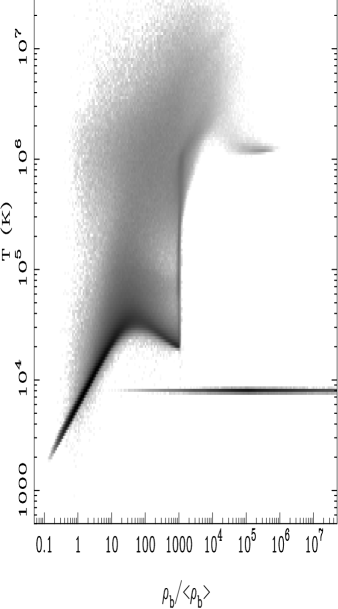
Figure 1.— Density–temperature phase diagram for the simulation, at redshift $z=3$.

In Figure 1, we show a phase diagram of temperature vs. density for particles in the simulation at $z=3$, with a grayscale weighted by mass. We have plotted separately the two gas components of the particles which have formed stars. The cold dense cloud component can be readily seen at the bottom of the plot. Most of the mass in galaxies is in these clouds, whereas much of the volume of the ISM is occupied by the hot phase, which has a temperature of close to $10^{6}$ K and can be seen near the top right of the plot.

Most of the mass in the universe as a whole, however is contained in the diffuse IGM, at or around the mean density. The locus which contains this gas is in the bottom left corner, where we can see a tight relation between temperature and density (see e.g. Katz et al. 1996, Hui & Gnedin 1997):

$$T=T_{0}\left(\frac{\rho_{b}}{\overline{\rho_{b}}}\right)^{\alpha}.$$ (1)

In this simulation, $T_{0}\simeq 6000$K and $\alpha\simeq 0.6$. Both parameters depend on the reionization history of the gas. If we take a random particle in the simulation and use its density $\rho_{b}/\overline{\rho_{b}}$ to predict its temperature $T$ using Eqn. (1), we find that $68\%$ of the mass in the simulation has an actual $T$ within $50\%$ of this predicted value ($61\%$ within $25\%$). This gas is responsible for most of the Ly$\alpha$ forest absorption (see Davé et al. 1999 for a detailed study). The scatter about this relation, while small, is partly due to noise from the SPH density estimates affecting the cooling rates (Springel & Hernquist 2002).

A shocked plume of hot gas occupies space in the top left part of the plot. This gas has been heated by shocks in IGM filaments and by falling into potential wells, where it is compressed and passes through accretion shocks, leading to virialization. Because the effective temperature of the hot ambient phase of the ISM was fixed at $\sim 10^{6}$ K in the multi-phase model used here, some hot ISM gas is able to escape from small halos and into the IGM, contributing to this hot plume of gas. The feedback processes modelled by the simulation therefore have the potential to influence the IGM close to galaxies, apart from affecting the star formation rate of the collapsed gas itself. However, we will see below that these effects on the IGM are rather modest. In §5 we will add some extra, much more extreme feedback to the simulations ‘by hand’ using simple models.

We use one other simulation for some tests in §2.2 below. It was run using the same cosmological model, but without star formation. In this simulation, gas cools and clumps to very high density in objects which would form galaxies, but the IGM properties are largely unaffected by the lack of star formation. The mass resolution of this simulation is slightly worse ($2\times 224^{3}$ particles, gas particle mass $3.6\times 10^{7}\,{\rm M_{\odot}}$), and the box size is the same as for our multiphase run.

2.1. Galaxy selection

Galaxy selection was carried out using a two step algorithm. We first identified groups of particles using a friends-of-friends algorithm (e.g., Davis et al. 1985) with a linking length of 0.15 times the mean interparticle separation. Embedded in each of the halos thus found, there can be one or several luminous galaxies, each consisting of stars, dense and diffuse gas, and dark matter. We thus split the halo candidates further into gravitationally bound ‘subhalos’ using a modified version of the algorithm SUBFIND (Springel et al. 2001). Note that due to the large size of the simulation, we had to fully parallelize both these group identification algorithms in order to be able to take advantage of the combined memory of several PC workstations.

After the group identification process has been carried out, we are left with a list of $\sim 40000$ galaxies with baryonic (gas + star) masses greater than $M_{b}=2\times 10^{8}{\rm M_{\odot}}$, although only $33000$ of them already contained independent star particles. When we use all galaxies in this list, it should be borne in mind that the list will not be $100\%$ complete, i.e. it will not contain all the galaxies above our mass detection threshold which would have been identified if we had much better mass resolution. A conservative limit for completeness is about 64 particles in total (see e.g., Gardner 2001), corresponding to $M_{b}=5\times 10^{8}\,{\rm M_{\odot}}$ in our case. For some of our work we will use all the galaxies, although most of our results will focus on galaxies above a much higher mass threshold, where completeness is expected to be very good. For example, with a mass-cut of $M_{b}=2\times 10^{10}\,{\rm M_{\odot}}$, there are 405 galaxies in the volume, so that the galaxies have space density $1.1\times 10^{-2}\;h^{3}{\rm Mpc}^{-3}$, which is similar to the value for local $L_{*}$ galaxies, and somewhat higher than the value for LBGs if the geometry of a $\Lambda$CDM universe is assumed.

The properties which are available to us after we have constructed our list of galaxies are their stellar, baryonic and dark matter masses, their instantaneous star formation rates (SFR), and their positions and velocities. The space density of LBGs in the samples of Steidel and collaborators (see e.g., Adelberger et al. 1999) is $\sim 10^{-3}\,\;h^{3}{\rm Mpc}^{-3}$ for the $\Lambda$CDM geometry. The simplest assumption to make is that LBGs correspond to the most massive galaxies that have formed by redshift $z=3$, and we will do this when calculating some of our results. With a lower mass cut of $M_{b}=10^{11}\,{\rm M_{\odot}}$, there are 30 galaxies in the simulation, so the observed space density is approximately reproduced. We can also select galaxies on the basis of a lower limit in SFR. As the simulation does not have sufficient resolution to capture brief intense starbursts which result from galaxy mergers (e.g., Mihos & Hernquist 1996; Hernquist & Mihos 1995), selecting on the basis of SFR effectively chooses galaxies with high quiescent star formation, which yields a catalog close to that obtained by choosing on the basis of mass. We give the space density of galaxies in the simulation for some values of the baryonic mass cut in Table 1 and SFR in Table 2.

Table 1The space density of galaxies, mean galaxy baryonic and total mass, and mean SFR, in the simulation as a function of lower baryonic mass cut.

$M_{b}$ cut	$\langle M_{b}\rangle$	$\langle M_{tot}\rangle$	$\langle$ SFR $\rangle$	Space den.
(${\rm M_{\odot}}$)	(${\rm M_{\odot}}$)	(${\rm M_{\odot}}$)	(${\rm M_{\odot}}/yr$)	$\;h^{3}{\rm Mpc}^{-3}$
$2\times 10^{8}$	$2.0\times 10^{9}$	$1.2\times 10^{10}$	0.24	1.0
$1\times 10^{9}$	$4.2\times 10^{9}$	$2.6\times 10^{10}$	0.59	0.39
$1\times 10^{10}$	$2.7\times 10^{10}$	$1.7\times 10^{11}$	6.0	0.028
$2\times 10^{10}$	$4.7\times 10^{10}$	$3.0\times 10^{11}$	12.5	0.011
$1\times 10^{11}$	$1.7\times 10^{11}$	$1.1\times 10^{12}$	40.7	$8.0\times 10^{-4}$

Table 2The space density of galaxies, mean galaxy baryonic and total mass, and mean SFR, in the simulation as a function of lower SFR cut.

SFR cut	$\langle M_{b}\rangle$	$\langle M_{tot}\rangle$	$\langle$ SFR $\rangle$	Space den.
(${\rm M_{\odot}}/yr$)	(${\rm M_{\odot}}$)	(${\rm M_{\odot}}$)	(${\rm M_{\odot}}/yr$)	$\;h^{3}{\rm Mpc}^{-3}$
0.03	$2.9\times 10^{9}$	$1.8\times 10^{10}$	0.39	0.63
0.1	$4.9\times 10^{9}$	$3.0\times 10^{10}$	0.71	0.32
1	$3.0\times 10^{10}$	$1.9\times 10^{11}$	8.2	0.020
10	$5.8\times 10^{10}$	$3.7\times 10^{11}$	21	$5.8\times 10^{-3}$

One additional sample of galaxies which we use is a set of merger remnants. The selection of these objects, and their properties are described fully in Westover et al. (2002, in preparation), which also deals in more detail with the properties of galaxies in this simulation, and their large scale clustering. Briefly, the merger remnants are defined to be galaxies which contain particles which were in at least two separate galaxies at $z=4$. These progenitors were selected from the $z=4$ simulation output using the same parallel groupfinder, and were required to contain at least 64 particles each.

                                                                            

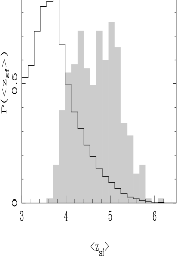
Figure 2.— The probability distribution of the mean redshift of star formation for galaxies in the simulation, at redshift $z=3$. The histogram in outline shows results for all 33000 galaxies in the simulation volume which contain stars, and the shaded histogram is for the 405 galaxies with baryonic masses larger than $2\times 10^{10}\,{\rm M_{\odot}}$.

In the simulation, star formation is occuring vigorously at the $z=3$ output time which we focus on. Information on the SFRs for galaxies of different masses can be read from Table 1. Later on, when implementing our models for extra feedback, we will need to know how long star formation has been proceeding for each galaxy. For each of the galaxies, we have calculated the mean redshift of star formation, weighted by stellar mass. A histogram of results is shown in Figure 2, for two different mass cuts: all galaxies, and galaxies with $M_{b}>2\times 10^{10}{\rm M_{\odot}}$. We can see that galaxies which are massive at $z=3$ formed most of their stars earlier than the small galaxies, as we would expect in a hierarchical universe where large structures are assembled from small ones. The mean redshift of star formation for the massive galaxies is $z=4.75$, whereas it is $3.75$ for all galaxies. It is interesting that none of the large galaxies formed most of their stars within the previous $\Delta z\simeq 0.5$, or $\sim 0.4$ Gyr. The bulk of winds generated by stars in these galaxies will thus be relatively old by $z=3$.

2.2. Lyman-alpha forest spectra

Ly$\alpha$ forest spectra were extracted from the simulation by integrating through the SPH particle kernels along randomly chosen lines of sight parallel to the axes of the simulation box. The neutral hydrogen density in pixels was convolved with the line-of-sight velocity field in order to generate realistic spectra. The procedure, which was carried out using the software package TIPSY, is decribed in more detail in Hernquist et al. (1996). Owing to its large size, the simulation data could not be analyzed at once on a single processor, so that it was necessary to modify the standard software. In this section, we present results from 500 spectra taken along each axis. In section 5, where different models are being tested, we restrict ourselves to analyzing 180 spectra in total for each model.

The simulation outputs at $z=3$ were used, both for the run with star formation, and for the smaller simulation without star formation employed for comparison. The effective UVBG intensity was adjusted slightly after the spectra were extracted, by multiplying the optical depths for Ly$\alpha$ absorption ($\tau\propto 1/I$, where $I$ is the radiation intensity) with a correction factor. This was done such that the mean flux level $\left<F\right>=\left<{\rm e}^{-\tau}\right>$ in the spectra was equal to the observed value. In the tests involving the Ly$\alpha$ forest alone, such as those in this section, we take the observed value to be $\left<F\right>=0.684$, as measured at $z=3$ from a sample of Keck HIRES spectra by McDonald et al.  (2000). For the simulation with star formation, the mean UVBG necessary to achieve this was 1.16 times the value actually used when the simulation was run, and 1.15 times for the run without.

When comparing to the data of A02, we use a different value of the mean flux $\left<F\right>=0.639$. With this value we approximately match the mean flux found by A02 at a separation of $1000{\rm\;km\;s^{-1}}$ from galaxies (§4) . This value (0.639) is the overall mean flux measured at $z=3$ by Press, Rybicki & Schneider (1993). To achieve this value, we lowered the UVBG to 0.85 times the intensity used when running the simulation. As the Press ${\rm et~{}al.\ }$ mean flux differs from the McDonald ${\rm et~{}al.\ }$ value, the level of UVBG radiation needed seems to be uncertain at least at the $\sim\pm 15\%$ level. The actual overall mean flux found by A02 is actually higher (0.67). The fact that we match their data with a lower value is probably due to finite simulation box size effects (we discuss this further in §4).

                                                                            

Figure 3.— The probability distribution of flux for simulations with and without star formation. The observational results of McDonald et al. (2000), also at $z=3$, are shown as points with error bars. No attempt to continuum-fit the simulation spectra was made, so that systematic errors in fitting the observations account for at least part of the difference between simulations and observations (see McDonald et al. 2000).

We have seen that including star formation in the simulation hardly affects the mean value of Ly$\alpha$ forest absorption. The mean UVBG intensity needed to match the observations differs by less than $1\%$. In Figure 3, we show the probability distribution function of flux values in the spectra for the two simulations and for the observational results of McDonald et al. (2000). There are marginal differences between the two theory curves. These may be attributable to differences in resolution between the two simulations, as they occur in low absorption pixels of the spectra, which are likely to be far away from the effects of star formation. There does not seem to be any dramatic effect on the absorption from hot gas which has been forced out of galaxies by feedback, and which can be seen on the phase diagram (Fig. 1). We have plotted the location of this gas and find it to be confined very close to galaxies. It has a very small volume filling fraction, not large enough to affect the Ly$\alpha$ spectra. Both simulation curves match the observations reasonably well, although it is hard to make an accurate comparison because there are uncertainties involved in estimating the true quasar continuum (the $F=1$ level) in the observations. McDonald et al. (2000) have attempted to estimate the possible effect of continuum fitting errors by modelling the procedure on theoretical spectra. They find that continuum fitting can change the distribution of flux values at high $F$ values noticeably, so that our simulations are likely not inconsistent with the data.

                                                                            

Figure 4.— The one-dimensional power spectrum of flux for simulations with and without star formation (lines). The observational results of McDonald et al. (2000), and Croft et al. (2002), both also for $z=3$, are shown as points with error bars.

The clustering properties of flux in the spectra can be measured using the one dimensional power spectrum of the flux, $P_{F,1D}(k)=\left<\delta^{2}(k)\right>$, where

$$\delta(k)=\frac{1}{2\pi}\int\delta(x){\rm e}^{-{\rm i}kx}{\rm d}x,$$ (2)

and which we measure using an FFT. Results are shown in Figure 4, for the same simulations and observations as in Figure 3, as well as the observational data of Croft et al. (2002). As with the flux probability distribution function, we can see that differences between the two simulations are generally small. Star formation and feedback here may be suppressing clustering very slightly on large scales, but the higher $P_{F,1D}(k)$ on small scales is probably due to the higher resolution of the star formation simulation. Both simulations match the clustering of the observational flux reasonably well, although their amplitude is slightly high. The turnover on small scales is most sensitive to the temperature of the IGM (e.g., White & Croft 2000, Theuns et al. 2000). From Figure 1, we can see that the temperature at the mean density is $\sim 6000\,{\rm K}$, which is low compared to observational Voigt profile fitting results (Schaye et al. 2000, McDonald et al. 2001).

3. Galaxy-IGM properties

We now examine the IGM around galaxies in the simulation. In Figure 5, we show panels centered on four different galaxies. Two of the galaxies have baryonic masses $M_{b}\simeq 10^{9}{\rm M_{\odot}}$, and the other two have $M_{b}\simeq 10^{11}{\rm M_{\odot}}$. These examples were chosen at random from the set of galaxies with masses close to theirs (within $20\%$). In the three panels on the right of each row, the SPH smoothing kernels have been used to assign the gas density, the gas temperature, and the stellar density to a grid of pixels. Note that the plots contain particles in a slice of thickness $2\;h^{-1}{\rm Mpc}$, for which we show the projected density in units of the mean.

                                                                            

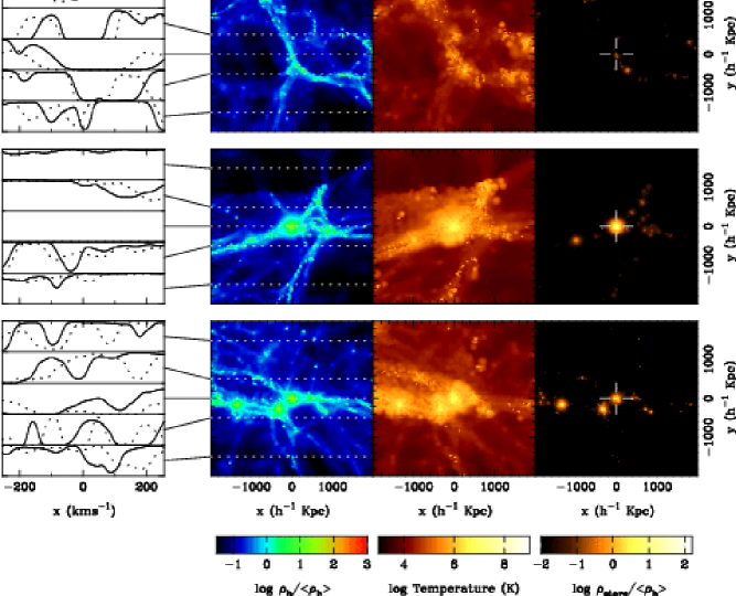
Figure 5.— Rightmost three panels in each row: the gas density, gas temperature, and stellar density in small regions (the slices are $2\;h^{-1}{\rm Mpc}$ thick) centered on galaxies in the simulation. The leftmost panel shows Ly$\alpha$ absorption spectra extracted along the lines of sight which are indicated as dashed lines in the density panel. The solid spectra are the full result, while the dotted spectra have been calculated with the peculiar velocities set to zero. The top two rows show results for two small galaxies (baryonic mass $\simeq 10^{9}{\rm M_{\odot}}$) and the bottom two rows are for much more massive galaxies (baryonic mass $\simeq 10^{11}{\rm M_{\odot}}$).

If we first examine the plots of gas density, it appears that the small galaxies lie along filaments, like strings of beads, whereas the massive objects tend to be found at filament intersections. The mass distribution around the massive galaxies is often strongly anisotropic outside the central $\sim 100h^{-1}{\rm kpc}$. Later, we will be computing spherically averaged quantities such as the density, temperature and absorption profiles around galaxies. It is therefore worth bearing in mind that the underlying morphology of the gas around galaxies may influence this.

The panels showing gas temperature are mass-weighted, as we first assign $\rho_{b}T$ to the pixels before dividing out $\rho_{b}$. The gas closest to the galaxies has a temperature of about $10^{5}\,{\rm K}$ for the small objects and $2\times 10^{6}\,{\rm K}$ for the large galaxies. This corresponds to thermal virial velocities of $40{\rm\;km\;s^{-1}}$ and 160 ${\rm\;km\;s^{-1}}$, respectively. Although many of the particles are multiphase, we only count the temperature of the hot component when making the plot. When we come to calculate the absorption by neutral hydrogen, we will not include the effect of the cold clouds in galaxies either. As the clouds have a cross section for absorption themselves, our results will constitute a lower limit on the absorption. In any case, the absorption closest to galaxies is subject to several uncertainties, not least the effect of feedback from winds, and this is what we shall model in most detail.

In the plots of stellar density in Figure 5, we can see more clearly where the galaxies actually lie. Both massive galaxies are in small groups, and even the smaller galaxies have some companions with similar masses.

The leftmost panels in each row of Figure 5 show the Ly$\alpha$ forest absorption along quasar sightlines taken through the box at three different impact parameters from the galaxies: $0$, $500$, and $1500\,h^{-1}{\rm kpc}$. We also draw separate curves for spectra generated along the same sightlines after setting the peculiar velocities to zero. By comparing these spectra to the temperature plots, we can see that there is neutral hydrogen present and causing absorption even when the gas is hot (the neutral fraction is $\sim 10^{-6}$ in the $\sim 10^{6}\,{\rm K}$ gas close to the large galaxies). We notice that neither the shock heating from virialization or the feedback from SN in the galaxies has cleared out a void in the absorption. The absorption becomes noticeably weaker in the sightlines which have largest impact parameters, even for the smallest galaxies. We will see later that there is indeed a substantial enhancement in absorption within $1-2\;h^{-1}{\rm Mpc}$ of most galaxies.

When integrated along the portions of spectra plotted, the lines of sight which have zero impact parameter yield neutral hydrogen column densities of between $N_{\rm HI}=4\times 10^{15}{\rm cm}^{-2}$ (the first galaxy) and $N_{\rm HI}=10^{17}{\rm cm}^{-2}$ (the third galaxy). No self-shielding corrections have been applied when calculating the neutral fraction, which could therefore be higher. Although the escape fraction for ionizing photons from LBGs has recently been found to be large (Steidel et al. 2001), we expect that local photoionizing radiation from stars is unlikely to modify the absorption properties of this gas (see §5.1).

                                                                            

Figure 6.— The mean volume-weighted densities (panel [a]) and temperatures (panel [b]), averaged around galaxies in real space at $z=3$. Results are shown for different lower galaxy baryonic mass limits, as well as for dark matter particles as centers, and for galaxies which are merger remnants (see text, §2.1 for definition).

In order to examine IGM trends with galaxy properties more quantitatively, we now average the temperature and density around different sets of galaxies. We use the same sightlines that were used to make Ly$\alpha$ forest spectra, and again integrate through the SPH kernels to find the gas density and temperature in pixels (this time in real space, without peculiar velocities). Looping through the list of galaxies, we measure the distance from the center of each galaxy to each pixel, in ${\rm\;km\;s^{-1}}$. In our $\Lambda$CDM cosmology, at $z=3$, each comoving $\;h^{-1}{\rm Mpc}$ corresponds to 112 ${\rm\;km\;s^{-1}}$ along the line of sight. We convert distances across and along the line of sight (sometimes referred to as $\sigma$ and $\pi$) to ${\rm\;km\;s^{-1}}$. The pythagorean galaxy-pixel distance is the quantity $\Delta_{r}$ plotted on the $x$-axis of Figure 6. As we calculate the mean density at each radius by summing the density in pixels and dividing by the number of pixels, the results are essentially volume-weighted.

In Figure 6, we show the results for galaxies with different lower mass limits. There is a general trend whereby higher mass galaxies are found in regions of higher density, although the trend with galaxy mass is weak. The profile of density with radius stays approximately the same in terms of its shape, but the amplitude varies like $\rho\propto M_{b}^{0.3}$. The galaxies which are merger remnants (see §2.1) have a mean baryonic mass of $M_{b}\simeq 1.6\times 10^{10}\,{\rm M_{\odot}}$ and appear to reside in similar density environments as other galaxies of comparable mass.

The density profile around randomly chosen dark matter particles is also shown in Figure 6. Interestingly, although on large scales the dark matter has lower density and temperature profiles than the lowest mass galaxies, within $\sim 100{\rm\;km\;s^{-1}}$ the profiles rise significantly. There therefore appears to be some sort of antibias of galaxies relative to dark matter on the smallest scales. We shall see later that this also manifests itself in small scale clustering measured using the correlation function. The temperature profiles all flatten off to the mean volume-weighted value, which is $17000\,{\rm K}$.

                                                                            

Figure 7.— The mean volume-weighted densities (panel [a]) and temperatures (panel [b]), averaged around galaxies in real space at $z=3$. Results are shown for different lower galaxy star formation rates, as well as for dark matter particles as centers, and for galaxies which are merger remnants, and which also have star formation rates above a threshold of $1\,{\rm M_{\odot}}\,{\rm yr}^{-1}$ (see text for definition).

If instead we rank the galaxies by their instantaneous SFRs, there is also a weak trend of increasing density and temperature close to galaxies, as seen in Figure 7. In this plot, we show results for a population of merger remnants slightly different from that used in Figure 6. Here we take only those merger remnants with a SFR $>1\,{\rm M_{\odot}}/{\rm yr}$, which is $25\%$ of the merged population. Again, the mergers have similar properties to the other galaxies with the same SFRs (in fact, the populations largely overlap, so this is not suprising).

Taking a slightly different approach, we refer to the density-temperature phase diagram of Figure 1, and to Equation (1). If we look at galaxies with masses $M_{b}>2\times 10^{10}\,{\rm M_{\odot}}$, $3.4\%$ of the volume of the universe (and $13.5\%$ of the baryonic mass) lies within $0.1-1\;h^{-1}{\rm Mpc}$ ($11-110{\rm\;km\;s^{-1}}$ in velocity units) of least one of them. Of this gas, only $40\%$ by mass lies within $50\%$ in $T$ of the locus defined by Equation (1). Within $100\,h^{-1}{\rm kpc}$, only $7\%$ of the gas lies on the tight $\rho-T$ relation. The situation for smaller galaxies follows a similar pattern, but obviously there is much less space that is at least $1\;h^{-1}{\rm Mpc}$ away from any galaxy. For all galaxies in the box, only $33.2\%$ of the volume, and $12.4\%$ of the baryonic mass satisfies this latter condition (being far from all galaxies), and $99.5\%$ of the associated gas mass lies on the $\rho-T$ relation.

We expect the neutral fraction in gas close to galaxies to decline because of the collisional ionization that occurs at high temperature. However, the total density of material increases nearby, and the recombination rate increases, both effects increasing the neutral density. We can calculate roughly what we might expect to happen to the Ly$\alpha$ absorption if we consider that gas far from galaxies has a mean temperature of $\sim 20000\,{\rm K}$, and a density $\sim 5-10$ times less on average than gas within $100{\rm\;km\;s^{-1}}$. The low temperature gas is almost totally photoionized (see Katz et al. 1996, Croft et al. 1997, Figure 1), and has a neutral fraction of $\sim 4\times 10^{-6}$. The gas close to massive galaxies is largely collisionally ionized and has roughly the same neutral fraction, which for collisional ionization only depends on temperature, and not on density. The optical depth for Ly$\alpha$ absorption, being proportional to the neutral hydrogen density will be roughly $5-10$ times higher within $100{\rm\;km\;s^{-1}}$ of galaxies. Note that the recombination rate, and hence the neutral fraction in the latter case varies like $T^{-0.7}$. If we wanted to change the temperature so that the Ly$\alpha$ optical depth would be the same close to galaxies as far away from them, we would thus need to raise $T$ by a factor of $\sim 10-30$. We will explore these issues in §4 and §5 in more detail.

4. Galaxies and the Lyman-alpha forest

We take the Ly$\alpha$ forest spectra extracted from the simulations as described in §2.2, and average the flux in pixels at different distances from galaxies. The results for the mean flux are show in Figure 8. The quantity shown is defined by

$$\left<F\right>(\Delta_{r})=\frac{1}{N(\Delta_{r})}\sum^{N(\Delta_{r})}_{i=1}F_{i},$$ (3)

where $N(\Delta_{r})$ is the number of pixels at distance $\Delta_{r}$ ($\pm$ a bin width) from a galaxy. We also plot the standard deviation of pixel values about the mean curve,

$$\sigma_{F}(\Delta_{r})=\left[\frac{1}{N(\Delta_{r})}\sum^{N(\Delta_{r})}_{i=1}[F_{i}-\left<F\right>(\Delta_{r})]^{2}\right]^{\frac{1}{2}}.$$ (4)

The same lines of sight are used that went into the computation of the density and temperature profiles in the previous section, except that the results are now in redshift space.

                                                                            

Figure 8.— (a) The mean Ly$\alpha$ forest flux averaged in pixels at different distances from galaxies in the simulation (at $z=3$). Results are shown for different lower galaxy baryonic mass limits, as well as for dark matter particles as centers, and for galaxies which are merger remnants (see text for definition). The observational results for the LBGs of Adelberger et al. (2002) are shown as points. (b) The standard deviation of Ly$\alpha$ forest flux values about the mean curves shown in panel (a). Again, we show results for pixels at different distances from galaxies.

We saw in §3 that the temperature and density close to galaxies both increase for increasing galaxy mass. In Figure 8a, where we show the average flux as a function of $\Delta_{r}$, this translates to a monotonic relationship between absorption and galaxy mass. The increase in density is more important than the increase in collisional ionization that accompanies higher temperatures, and so more massive galaxies have more associated absorption. Interestingly, the absorption profiles around dark matter particles are the weakest, even though the nearby real space densities around the smallest galaxies are smaller than for randomly chosen dark matter. This may have to do with the fact that the Ly$\alpha$ forest profiles are affected by infall velocities, which we will explore briefly below.

As with their density profiles, the merger remnants have similar absorption as the set of all galaxies of the same mass. Figure 8a corresponds to a mean profile around many galaxies. Interpreting this as a single profile around an average galaxy is misleading (we show below that the dispersion around this profile is large), even though its shape is suggestive of a Voigt profile, with a wide damping wing. As we have seen from the density profiles, however, this is more likely to come from the density enhancement on large scales that results from clustering.

Recently, observational results have become available for the quantity $\left<F\right>(\Delta_{r})$, and on Figure 8a we show the data of Adelberger et al. (2002). The points were calculated from a set of 7 fields containing both QSOs and LBG galaxy candidates. 431 LBGs with redshifts were used in the study, and Ly$\alpha$ forest spectra were obtained for 8 QSOs with redshifts spanning $3.1<z<4.1$. The error bars on the measured $\left<F\right>(\Delta_{r})$ values represent the error on the mean obtained from the scatter between fields.

We can see that the simulations are consistent with the observational result for scales $\Delta_{r}>250{\rm\;km\;s^{-1}}$. This is mainly because we have normalized the UVBG intensity to match the Press et al. mean flux measurements, which also reproduces the A02 mean flux versus distance measurements on the largest scales we plot. The most massive simulation galaxies offer a better fit on these scales than the others. Because the simulation is not much larger than the largest scale in Figure 8a, the flux recovers to the mean more quickly than if larger scale modes were present. Because of this, to match the A02 data we have used a slightly lower mean overall mean flux than A02 found themselves.

On small scales, however, the finite box size will not cause uncertainties. The discrepancies we see there are real, where the observed mean flux actually rises below distances of $200{\rm\;km\;s^{-1}}$, signifying a lowering of the mean absorption as we get closer to galaxies. As this is opposite to what is seen in the simulations, it is quite surprising, and we will devote a substantial part of the rest of this paper to studying possible causes for this.

We note here that the measurement of the absorption profile close to galaxies is extremely difficult observationally, due to the velocity differences between different estimates of the galaxy redshift. For example, the redshift difference between interstellar lines and the Ly$\alpha$ emission line often exceeds 750 ${\rm\;km\;s^{-1}}$. According to A02, the best estimate of the redshift of stars in a galaxy should come from the nebular lines due to hot gas associated with stars. As these nebular lines were only available for a minority of galaxies, A02 had to resort to an estimate of the nebular line redshift derived from UV spectral characteristics for the others. The A02 result shown in Figure 8a is therefore tentative, as additional redshift uncertainties might smooth out any absorption dip. In §5.2, we will quantitatively examine an extreme version of this effect in the simulation by estimating the galaxy redshift from material that has the wind velocity.

Here, we will make use of A02’s estimates of the redshift uncertainty. We do this by recalculating the results after adding a random velocity to the redshift of each galaxy, in order to gauge the effect of the uncertainty. A02 estimate that an optimistic value for the galaxy redshift uncertainty is given by a Gaussian standard deviation of $\sigma_{v}\sim 150{\rm\;km\;s^{-1}}$ ($\sigma_{z}\sim 0.002$). A02 also note that there will in general be a long tail to this distribution, with a few outliers corresponding to very discrepant results. We have not modelled this, but restricted ourselves to a value of $\sigma_{v}\sim 150{\rm\;km\;s^{-1}}$, as well as trying $\sigma_{v}\sim 300{\rm\;km\;s^{-1}}$. The results are shown in Figure 9, for two different mass cuts. We can see that although the velocity error does smooth out the absorption on small scales, the effect does not bring the simulations into good agreement with the data. For the most massive galaxies (which fit the absorption curves best on large scales) and with the A02 estimate of $\sigma_{v}$, the effect is not very large. In the rest of the paper, we will not convolve our simulation results with errors in this way, so we should bear in mind that the results on small scales may be uncertain to the level shown in Figure 9.

                                                                            

Figure 9.— (a) The mean Ly$\alpha$ forest flux averaged in pixels at different distances from galaxies in the simulation (at $z=3$), for galaxies above two different mass cuts. The observational results for the LBGs of Adelberger et al. (2002) are shown as points. In this plot, we have added Gaussian velocity errors with a standard deviation $\sigma_{v}$, as indicated, in order to gauge the effect of uncertainty in the galaxy redshifts. (b) The standard deviation of Ly$\alpha$ forest flux values about the mean curves shown in panel (a). Again, we show results for pixels at different distances from galaxies.

The variance around the mean profile is shown in Figure 8b (we actually plot the standard deviation $\sigma_{F}$). We might expect this quantity to be lower around more massive galaxies in the simulation, as they are more likely to always be accompanied by a large amount of absorption. We can think of this statistic as probing the stochasticity of the relationship between Ly$\alpha$ absorption and galaxies. In the plot, the dark matter particles are indeed accompanied by a larger variance on small scales, and the most massive galaxies have the least.

The curves rise to a maximum of $\sigma_{F}=0.35$ at $\Delta_{r}\simeq 150{\rm\;km\;s^{-1}}$ and then fall gradually back to a value of $0.32$ at $1000{\rm\;km\;s^{-1}}$ separation. The shape of this function is presumably related to the fact that within 150 ${\rm\;km\;s^{-1}}$ or so of galaxies much of the absorption is saturated, so that only a small variance in the flux is possible. On slightly larger scales, the variance of optical depth about the mean is smaller, but most absorption is in the optically thin regime, and so the variance in the flux is large. The variance of the optical depth then decreases further on larger scales. A02 have not published this quantity, but the authors were kind enough to provide preliminary datapoints (Adelberger, private communication). The observational data follows the same trend, with possibly less variance on small scales. The exact value of this quantity is influenced observationally by variations in continuum fitting from quasar to quasar. These systematic errors will tend to boost $\sigma_{F}$, so that an accurate assessment of the uncertainties in $\sigma_{F}$ is difficult, and error bars have therefore not been plotted. We note that the statistical errors on $\sigma_{F}$ are likely to be at least as large than those on $\left<F\right>(\Delta_{r})$, so that any inferences we draw will not be very strong. We find that the values of $\sigma_{F}$ are slightly lower for the simulations on large scales, for all cuts in galaxy baryonic mass. On small scales, the fact that the observational $\sigma_{F}$ may be small seems to indicate that Ly$\alpha$ absorption and therefore the conditions in the IGM around the LBGs may not vary much from one galaxy to another.

                                                                            

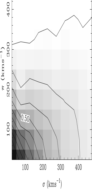
Figure 10.— The mean value of Ly$\alpha$ forest flux at different distances from galaxies (with a lower baryonic mass limit of $2\times 10^{10}{\rm M_{\odot}}$) in the simulation. We show results as a function of distance across the line of sight ($\sigma$) and along the line of sight ($\pi$). The contours are at intervals of 0.05, increasing from bottom left to top right, and the $F=0.5$ contour is labelled.

An alternative way to plot the Ly$\alpha$ absorption around galaxies is to break up the galaxy’s separation into distances across and along the line of sight ($\sigma$ and $\pi$). We show a contour plot of $\left<F\right>(\sigma,\pi)$ in Figure 10. The effects of peculiar velocities are clearly visible, including the squashing of contours on large scales by infall (Kaiser 1987), and the pushing of absorption contours along the $\pi$ axis due to random virial velocities close to galaxies. Such a plot might in principle be used to study the velocity field of IGM gas around galaxies at high redshift, or even to measure cosmic geometry (Alcock & Paczynski 1979), although problems with systematic errors would be considerable.

5. Simple models for extra feedback

The star formation model employed in the simulation already incorporates a simple model for feedback (§2). For each ${\rm M_{\odot}}$ of long-lived stars formed, an energy of $7.35\times 10^{48}$ ergs is assumed to be released by supernovae from massive stars, and is added as thermal energy to the ISM, which itself is modelled using multiphase particles. Because star formation proceeds in a relatively quiescent manner, the gas is heated up fairly slowly, and dramatic feedback-related effects do not seem to occur. In particular, the simulation does not show evidence of the strong winds from high-z galaxies which are seen observationally (e.g., Pettini et al. 2001). Ideally, one would like to model star formation more accurately, so that such features arise naturally. While some progress is being slowly made in this direction, there are still gaps in our understanding of the physics of star formation and feedback processes, which preclude a numerical modelling from first principles within cosmological volumes at present. In the meantime we can explore stronger feedback in a simplified way by modifying the outputs of our existing simulation after it has been run. In this section, we will try out some very crude, simple models of feedback processes that might be energetically possible, given the number of SN in each galaxy. We will explore the effect of these on the surrounding Ly$\alpha$ forest absorption, and how it might differ from that seen in §4. Also, the UVBG radiation might be inhomogeneous, and at least partly generated by galaxies. We will also briefly examine what consequences this might have.

The simulation we are using here has already been described in the previous sections. We are confident that much of the underlying IGM physics is correct, and also that the cosmological model, $\Lambda$CDM, is not far from the true one, given that it satisfies many observational constraints (e.g., Ostriker & Steinhardt 1995). The amount of gas which can cool and condense into galaxies is in principle a reliable prediction of simulations of this kind (Gardner et al. 2001, and Davé et al. 2000), although computations of this quantity are not without numerical subtleties (Springel & Hernquist 2002). However, the simulations probably provide an upper limit, given that feedback might prevent some condensations from occuring. While the thermal feedback already included in the simulations has substantial modelling uncertainty, the exact effects of the extra feedback we will add here is even more uncertain. For a start, we have already used up the available SN energy heating up the IGM and ISM gas when the simulation was running. In our simple models, we will therefore be assuming that this energy input has had little effect on the IGM, and that we are free to add it again to the simulation, but in a form where it can have more extreme consequences.

Our approach in this section of the paper is similar in spirit to the work carried out by Aguirre et al. (2001a,b,c). We will however be rather less sophisticated. Aguirre et al. found that modelling the escape of gas from the gravitational potential well of galaxies had the most importance in governing the effects of feedback. We will therefore treat this in a simplified manner, but we will not explicitly model the effects of ram pressure, radiation pressure, and the ambient thermal pressure. The effects of feedback on the Ly$\alpha$ forest have been previously explored by Theuns et al. (2001). Detailed theoretical calculations and simulations of the escape of winds from galaxies have been carried out by, amongst others, Ferrara et al. (2000), Ciardi & Ferrara (1997), Efstathiou (2000), MacLow & Ferrara (1999), and Murakami & Babul (1999).

                                                                            

Figure 11.— The four panels show different randomly chosen spectra through the box. The fiducial simulation is shown as a solid line, and two models with different types of feedback from galaxies added after the simulation was run are also shown. All spectra were calculated using the same mean UVBG intensity, but do not have the same mean absorption. The dashed line represents a kinetic feedback model in which IGM gas within a wind radius surrounding each galaxy (calculated on the basis of the potential well depth and assuming that 10% of the total supernova energy was available for the winds) was removed. The dotted line shows spectra extracted using the same gas density distribution as in the no extra feedback case, but with an inhomogeneous UVBG generated by the galaxies themselves. This line lies on top of the fiducial line almost everywhere. The filled points show the positions of galaxies within $200{\rm\;km\;s^{-1}}$ of the line of sight. The perpendicular distance from the galaxy to the line of sight determines its position along the $y$-axis (see scale on the right $y$-axis). The position along the line of sight in redshift space is the $x$-coordinate. The symbol area is proportional in size to the baryonic mass of the galaxy. The most massive galaxy shown has $M_{b}=10^{11}\,{\rm M_{\odot}}$.

                                                                            

Figure 12.— The one-dimensional power spectrum of flux for spectra with no extra feedback (lines), and with two variants of extreme feedback added to the IGM after the simulation was run (these are the same as those shown in Figure 11). The dashed line represents a kinetic feedback model in which IGM gas within a wind radius surrounding each galaxy was removed. The dotted line contains no winds but instead an inhomogenous photoionzing background radiation field generated by the galaxies themselves. The observational results of McDonald et al. (2000), and Croft et al. (2002), both also for $z=3$, are shown as points with error bars.

5.1. UV radiation proximity effect

As stated in §2, the simulation was run with a spatially uniform ionizing background, with a spectrum derived by processing QSO source radiation through the IGM (Haardt & Madau 1996). The mean free path of ionizing photons depends on the amount of neutral hydrogen, which increases rapidly towards high redshifts. At $z=3$, according to Haardt & Madau (1996), the attentuation length $r_{\rm att}$ (over which the flux decreases by ${\rm e}^{-1}$) is $\simeq 130\,h^{-1}{\rm Mpc}$ comoving for photons with a wavelength of 912 ${\rm\AA}$, assuming our $\Lambda$CDM cosmology. The fluctuations of the ionizing background will depend on this quantity, and on the space density of sources. For rare sources such as QSOs, the fluctuations will be largest, but take place over large scales. Fardal & Shull (1993), Zuo (1992), and Croft et al. (1999) showed that even in this case, we expect little effect on Ly$\alpha$ forest spectra at $z\sim 3$.

There is evidence that a portion (maybe substantial) of the UVBG arises from starburst galaxies rather than QSOs. Some flux beyond the Lyman limit has been seen in spectra of LBGs by Steidel et al. (2001), indicating that the escape fraction of ionizing photons from these galaxies may be significant. The implications for the overall level of the UVBG have been discussed by Haenhelt et al. (2001), Hui et al. (2002), and Sokasian et al. (2002). If the UVBG was generated by galaxies, fluctuations in its intensity would occur on smaller scales than with QSOs, but the UVBG should be smoother overall, as each point in space can “see” many sources. Making use of a model by Kovner & Rees (1989), Croft et al. (1999) estimated that sources with the space density of LBGs would result in the standard deviation of fluctuations being at the $\sim 10^{-3}$ level overall. However, the UVBG close to galaxies would obviously be of highest intensity, and it is possible that this “proximity effect” would decrease the nearby neutral fraction by a measurable amount.

In order to roughly gauge the effect on the profile of absorption around galaxies, we have tried replacing our uniform UVBG with point sources at the positions of galaxies in the simulation. This was done after the simulation was run, but before spectra were generated. We use the optically thin approximation, as the mean free path of photons is much larger at $z=3$ than our box size. At higher redhifts, this would not be the case, and simulations that follow reionization self consistently (e.g., Abel et al. 1999, Gnedin 2000, Ciardi et al. 2001, Sokasian et al. 2001) would become necessary. Here we assume that the fluctuations in the IGM neutral fraction at $z=3$ do not retain a strong memory of the earlier history of reionization (see Hui & Gnedin 1997, Gnedin 2000).

In our simple model, we take the total flux of ionizing radiation emitted by each source to be proportional to its instantaneous SFR. We keep the same UVBG spectral shape as before, which will not affect the HI neutral fraction, although with the softer spectrum of real galaxies one might expect other effects, such as less photoheating of the gas. Radiation from each individual source is allowed to shine on matter half a box length away, using the periodic boundary conditions, and then it is cut off sharply. As this is less than the attentuation length, we add a uniform UVBG component to account for galaxy sources farther away. To calculate this component, we use the fact that the total intensity of UVBG radiation, and hence the photoionization rate, at a point in space is proportional to $r_{\rm att}$. This is because the number of sources within the attentuation volume increases like $r^{3}_{\rm att}$, but they are dimmed like $r^{-2}_{\rm att}$. We therefore add a uniform BG with a photoionization rate

$$\Gamma_{\rm uniform}=\Gamma_{\rm gals}\frac{r_{\rm att}}{0.5\,B},$$ (5)

where $B$ is the simulation boxsize, and $\Gamma_{\rm gals}$ is the photoionization rate due to the sources. We estimate $\Gamma_{\rm gals}$ by Monte-Carlo integration, and take $r_{\rm att}$ to be a conservative $80\;h^{-1}{\rm Mpc}$ comoving. The uniform component of the UVBG is then $4.8$ times that from galaxies inside the volume. We do not use any other component for the UVBG, i.e., all of the UVBG is generated by galaxies.

Some example spectra generated using this inhomogenous UVBG are show in Figure 11 (the dotted line). The uniform case is also shown, and we can see that there is hardly any difference between them. As we might expect, the minute observable differences are only apparent in regions close to galaxies, which are shown on the plot with their impact parameter relative to the QSO line of sight on the $y$-axis. The galaxies are mainly concentrated around high absorption features in the spectra. The spectra shown as dashed lines in each panel correspond to a strong kinetic feedback model, which we will discuss in §5.3.

Overall, owing to their large number, the galaxy sources yield only small fluctuations in the Ly$\alpha$ forest absorption. We have also tried only using galaxies with high SFRs (e.g. ${\rm SFR}>10\,{\rm M_{\odot}}\ {\rm yr}^{-1}$), but it makes little difference. From our sample of spectra (180 lines of sight), we find that the overall UVBG intensity required is the same as in the uniform case. The flux-power spectrum $\delta_{F,1D}$ is shown in Figure 12, compared to that for the same 180 spectra with a uniform BG. There are only small differences, rising to $\sim 5\%$ on the largest scales.

                                                                            

Figure 13.— (a) The effect of thermal feedback (for this, only the temperatures of gas particles are changed, see text, §5.3) on the mean Ly$\alpha$ forest flux averaged in pixels at different distances from galaxies in the simulation (at $z=3$). All results are for the flux averaged around galaxies with baryonic masses $M_{b}>2\times 10^{10}\,{\rm M_{\odot}}$. The different curves are for different ways of adding the extra feedback, all computed after the simulation was completed. These are a model where $100\%$ of the SN energy in each galaxy was used to heat the surrounding IGM (thick solid line), and a similar model, but with 100 times the actual SN energy available being used (dashed line). The latter is not meant to represent a realistic model, but was just implemented in order to yield a noticeable effect. The dot-dashed line is for results with $100\%$ of the SN energy used, but with the redshift of the galaxy taken to be that of the wind (i.e. a difference of $600{\rm\;km\;s^{-1}}$ in this case). Finally, the dotted line is for no thermal feedback, but with the UV background radiation being entirely contributed by the galaxies in the simulation and hence being inhomogeneous (see 5.1). The observational results for the LBGs of Adelberger et al. (2002) are shown as points. In panel (b), we show the standard deviation of Ly$\alpha$ forest flux values about the mean curves shown in panel (a).

The mean Ly$\alpha$ forest flux averaged around galaxies with masses $M_{b}>2\times 10^{10}\,{\rm M_{\odot}}$ is shown in Figure 13, again compared to the same 180 spectra we computed for the uniform case. The LBG proximity effect is visible and has the right sign, but it only changes the mean flux close in by a maximum of $0.04$. Modelling the IGM taking into account regions where there will be an optically thick regime is unlikely to reconcile the simulation with observations, as such regions would tend to have more Ly$\alpha$ forest absorption anyway. We will describe below the other lines on Figure 13, which are for models of galactic winds.

5.2. Thermal feedback from winds

We will now try distributing SN energy among nearby particles that might be affected by large-scale winds from galaxies. Given the theoretical uncertainties involved in predicting the structure of a wind and its interaction with the IGM, we will just try simple examples of what might be energetically feasible. One possibility is that the energy from SN spread by a wind is turned into thermal energy in the IGM. Each ${\rm M_{\odot}}$ of stars releases $7.35\times 10^{48}$ ergs. We have already distributed this energy into the ISM represented by the multiphase particles. Here we will assume that somehow all of this energy is able to escape in the form of a wind and instead heats up the IGM at comparatively large distances. We will however not remove energy from the galaxy ISM particles, so that we are effectively adding extra SN energy.

Our model for such “thermal” winds is basic. We assume spherical symmetry, and a wind outflow velocity, $v_{\rm wind}$. For our fiducial case we set $v_{\rm wind}=600{\rm\;km\;s^{-1}}$, in the same range as the observational results of Pettini et al. (2000, 2001). We assume that the wind starts blowing from each galaxy at the mean redshift of SF of the particles in the galaxy (see Figure 2), and continues to $z=3$, without slowing down. In our model for thermal winds, we therefore do not include the effect of the gravitational potential well of the galaxy (no matter is moving, and only thermal energy is propagating outwards). We distribute the thermal energy so that the energy per unit gas mass in each particle is proportional to $1/r^{2}$, where $r$ is the distance from the particle to the galaxy center. The minimum radius from the center of each galaxy at which this feedback energy is added is set to be $10\,h^{-1}{\rm kpc}$. We also assume that all of this deposited feedback energy remains as thermal energy at $z=3$, without cooling, in order to achieve the maximum effect. In the interests of simplicity, we work with only one simulation output file (at $z=3$), and assume that galaxies do not move over the wind lifetime.

With $v_{\rm wind}=600{\rm\;km\;s^{-1}}$, we find that the outer radius of the wind around each galaxy averages $650\,h^{-1}{\rm kpc}$, with a maximum of $2\;h^{-1}{\rm Mpc}$. As this distance is governed by the mean $z$ of SF, large galaxies have the largest wind-affected volume around them because they are older. With this high velocity and the fact that winds do not slow down in the model, a very large volume of the Universe is affected ($60\%$ is filled by winds). If we reduce $v_{\rm wind}$ to $300{\rm\;km\;s^{-1}}$, we find a wind filling factor of $18\%$.

                                                                                       

Figure 14.— The volume-weighted temperature averaged around galaxies with with baryonic masses $M_{b}>2\times 10^{10}\,{\rm M_{\odot}}$, for different thermal feedback prescriptions (see §5.3, and the caption for Figure 13 for details). The dotted line (inhomogeneous UVBG) lies underneath the “no extra feedback” line.

The effect of the added thermal energy on the mean temperature of the IGM gas around galaxies is shown in Figure 14. In this plot, we show only results for the 405 most massive galaxies in the simulation ($M_{b}>2\times 10^{10}\,{\rm M_{\odot}}$). We can see that with $100\%$ of the SN energy added, the temperature close in, already high because of shock-heating, hardly changes compared to the no-wind case. Further out, the mean temperature rises by $\sim 10\%$. We have tried varying $v_{\rm wind}$ from $60{\rm\;km\;s^{-1}}$ to $600{\rm\;km\;s^{-1}}$ and changing the energy deposition law to $1/r^{3}$ but see little difference in the thermal structure. In order to see a large effect, we also tried adding 100 times the available SN energy to the IGM gas, which is obviously not a realistic model. The mean temperature then rises to a few times $10^{5}\,{\rm K}$. Also on Figure 14 is a line (hidden under the no feedback line) showing temperature profile results for the inhomogeneous UVBG model of §5.1. Here we have not added SN feedback energy, and temperature differences (which are too small to be visible) here only arise from differences in photoheating rates.

We now calculate Ly$\alpha$ forest spectra from the treated simulation output, along 180 randomly chosen lines of sight, the same that were used in the calculation of Figure 14. The mean UVBG intensity was varied in order to get the correct mean Ly$\alpha$ forest optical depth. For the feedback case where $100$% of the SN energy was used together with $v_{\rm wind}=600{\rm\;km\;s^{-1}}$, this intensity was the same as with no extra feedback. For $300{\rm\;km\;s^{-1}}$ winds, the effect of feedback removed a bit more absorption, so that the UVBG needed was $1\%$ lower. For the unphysical model where $100$ times the SN energy was used, the mean absorption level was drastically affected, and the UVBG had to be lowered to $48\%$ of its no-feedback value.

The resulting Ly$\alpha$ forest absorption profiles around massive galaxies are shown in Figure 13a. We can see that distributing the available SN energy as thermal energy has little effect on the absorption. It therefore seems likely that to achieve something with feedback we will need to physically displace gas surrounding galaxies or disturb its morphology (we will try this below). With $100$ times the SN energy used to heat the gas, the model is closer to the mean Ly$\alpha$ forest flux results of A02, but this model is obviously too extreme. Interestingly, the variance of the flux (Figure 13b) is lower at large separations in this unphysical model than in the other cases and in the observations.

Another line on Figure 13a shows what happens if we use the redshift of the wind as the redshift of the galaxy when calculating the galaxy-pixel separation. Basically, in this case we are subtracting $v_{\rm wind}=600{\rm\;km\;s^{-1}}$ from the galaxy position. Note that our modelling of this effect is probably too extreme, as the wind velocity will likely not have the same, high value for all galaxies. The effect of this offset is as one might imagine from looking back at Figure 10. If one centers the averaging around the galaxy on a point $600{\rm\;km\;s^{-1}}$ up the $\pi$ axis, the absorption dip will be missed. Something along these lines may be occuring in the observations, if the effect of wind velocities on the measured galaxy redshift has not been completely accounted for. Evidence against this being the whole story is the fact that, observationally, the flux rises close to galaxies (although this is only a $\sim 3\sigma$ effect), and the variance around the mean (Figure 10b) has the wrong shape for the wind-offset curve (note, however that this statistic has even larger observational uncertanties).

5.3. Kinetic feedback from winds

We have seen that our thermal wind model, which only changes the temperature of the IGM does not modify the neutral fraction by a sufficient amount to affect the Ly$\alpha$ forest. One can ask about a different model for feedback, in which winds physically displace gas in the IGM. In this section we study such “kinetic” winds and their effect on Ly$\alpha$ spectra.

Once again our model is extremely simple, and we make the assumption that the winds act in a spherically symmetric fashion around each galaxy. This time we will use the energy from SN to push baryonic material away from galaxies. For each galaxy, we find the gravitational potential energy necessary to move matter interior to a shell of radius $r_{\rm shell}$ to that radius:

$$E_{\rm GPE}=G\sum^{N}_{i=1}\left(\sum^{N_{i}}_{j=1}M_{j}\right)M_{i}\left(\frac{1}{r_{i}}-\frac{1}{r_{\rm shell}}\right)$$ (6)

where $G$ is the gravitational constant, $N$ is the number of gas particles interior to $r_{\rm shell}$, and $M_{i}$ is the mass of particle $i$ at radius $r_{i}$. $N_{i}$ is the number of gas particles interior to radius $r_{i}$. Here we ignore the expansion of the universe over the period of shell propagation. We also assume that all material within the shell is entrained, obviously the most extreme scenario possible.

In this simple model, we have a choice when deciding what to do with the IGM material affected by winds. The easiest scheme to carry out, and the most drastic, is to make all material inside the outer shell of the wind disappear. This will result in the evacuation of cavities in the IGM around each galaxy. As well as this scheme, we also try a second one, in which the particles are kept with the same SPH densities and temperatures, but placed at the shell radius. In order to avoid a shell profile which is very discontinuous, we smooth out the shell by adding a random radial displacement to each particle’s position, drawn from a Gaussian distribution with a dispersion of 10% of the shell radius. In carrying out this procedure, we go through the list of galaxies in a random order, one by one. Because of this, some gas particles are moved twice or more, allowing them to end up close to galaxies they had previously been moved away from.

As with the thermal wind scenario, the volume of space affected by winds can potentially be very large. Allowing $100\%$ of the available SN energy to move matter with kinetic winds results in a mean shell radius of $670\,h^{-1}{\rm kpc}$. This is quite close to the mean wind propagation radius for galaxies in the thermal wind case, where winds moved at $600{\rm\;km\;s^{-1}}$ without slowing down. For $100\%$ of the SN energy in kinetic winds we find that $62\%$ of the volume is affected by winds. Reducing the energy allowed to drive kinetic winds to $10\%$ results in a wind filling fraction of $28\%$. Even with only $1\%$ of the SN energy in kinetic winds, we still have $10\%$ of the volume filled by winds. We also tried the case where only the 400 most massive galaxies in the box are assumed to be able to drive winds. This resulted in a wind filling fraction of $8\%$ in the $10\%$ SN energy case.

                                                                            

Figure 15.— (a) The effect of kinetic feedback (see text, §5.3) on the mean Ly$\alpha$ forest flux averaged in pixels at different distances from galaxies in the simulation, at $z=3$. All results are for the flux averaged around galaxies with baryonic masses $M_{b}>2\times 10^{10}\,{\rm M_{\odot}}$. The different curves are for different ways of adding the extra feedback (see §5.3 for details). These are a model where $10\%$ of the available SN energy in each galaxy was used to evacuate a cavity in the IGM (thick solid line), and a similar model, but with only SN in the most massive 400 galaxies contributing to the feedback (dashed line) and the fraction of SN energy increased to $100\%$. Finally, the dotted line shows results when the mass in the cavity is redistributed in an arbitrary fashion rather than being eliminated. The observational results for the LBGs of Adelberger et al. (2002) are shown as points. In panel (b), we show the standard deviation of Ly$\alpha$ forest flux values about the mean curves shown in panel (a).

We can clearly see the effect of kinetic feedback on individual features in the spectra if we refer back to Figure 11. Here we have plotted the case where winds evacuate gas completely. Strong lines can be affected, and even if the galaxy involved is small, the absorption features are completely wiped out when the impact parameter is small enough.

Our results for the mean Ly$\alpha$ flux averaged around galaxies are shown in Figure 15. As with Figure 13, we only average around galaxies with baryonic masses $M_{b}>2\times 10^{10}\,{\rm M_{\odot}}$. We can see that, as we might expect, eliminating the mass within the shells rather than redistributing it has the largest effect. If this is done using $100\%$ of the SN energy (top curve), then there is much too little absorption compared to the observational data. With $10\%$ of the energy, there is still too little, but the results are more reasonable. However, the variance in the flux on small scales (bottom panel) does not match in this case.

If the matter is redistributed by winds, this can result in extra absorption at large ($>200{\rm\;km\;s^{-1}}$) distances from galaxies. In the particular case shown here, the redistribution results in a better match to observations on large scales than the case with no feedback. Of course, the mass redistribution within the feedback scheme is ad hoc, so that not too much should be read into this. It does however indicate that it is at least energetically possible for galactic winds to influence the absorption at some distance from galaxies, in both a positive and negative way. Mass moved by winds can increase the overall mean Ly$\alpha$ absorption, by moving material away from saturated regions. This could have important implications for the mean UVBG required to produce the observed level of absorption.

In the case plotted in Figure 11 ($10\%$ SN energy in winds), the UVBG must be changed by a factor 0.50 with respect to the no feedback case in order to match the Press et al. (1993) optical depth. If instead of eliminating the material within the wind radius, we redistribute it, we find that the UVBG intensity must be increased by 1.57 to match the Press et al. (1993) results. The effect of feedback in our simulations on the mean UVBG required is therefore uncertain. Whether the UVBG must be higher or lower depends on the absorption lines produced by winds and by the gas moved by them (see e.g., Theuns et al. 2001, Rauch et al. 2001, for the effects of lines from wind-blown shells). Our two kinetic feedback schemes are extreme, and are likely to bracket the possibilities. For comparison, our thermal-only feedback model (§5.2), which does not change the absorption by much, only requires a UVBG differing by $\sim 2\%$.

We have also calculated the power spectrum of the Ly$\alpha$ forest spectra for the kinetic wind model. The results are shown in Figure 12. Unlike the inhomogenous UVBG model, the kinetic wind feedback is able to change the flux power spectrum noticeably. Interestingly, this occurs on large scales rather than on small ones. Theuns et al. (2001) have noted that the distribution function pixel values of flux in simulations matches that from observed spectra very well, and concluded that this might be an indication that feedback is not very important. This argument may also apply to the power spectrum. On the other hand, it may be an indication that the flux power spectrum would be different without feedback, and the agreement is just a coincidence. If this were the case, then the recovery of the power spectrum of matter fluctuations from the Ly$\alpha$ forest flux power spectrum (e.g., Croft et al. 2002) could be affected.

To summarize this section, among the three different methods we have tried (UVBG proximity effect, thermal winds, and kinetic winds), only kinetic winds can potentially have important consequences. If SN energy in the form of winds is able to escape from galaxies, and sweep up shells of material (not just heating it it up), then the absorption properties of the IGM within $\sim 1\;h^{-1}{\rm Mpc}$ of galaxies can be significantly altered. The apparent deficit of absorption close to Lyman-break galaxies observed tentatively by A02 could be due to such winds, as suggested by those authors. We have seen in this section that such a scenario is energetically plausible in a $\Lambda$CDM universe.

5.4. Absorption and selection effects

Rather than LBGs acting on their environments, it is possible that instead the environment acts on the selection of LBGs themselves. For example, let us suppose that the density in dust in the IGM close to galaxies is linked to the strength of Ly$\alpha$ absorption. Galaxies with little dust obscuration will preferentially be selected to appear in a magnitude limited sample. These galaxies will then have little Ly$\alpha$ absorption close to them. If such a selection effect is strong enough, then it could conceivably account for the deficit of absorption close to galaxies seen by A02. In this case, the galaxies in the LBG sample may also have different clustering properties to the galaxy population as a whole.

We explore such a scenario in our simulation by taking the set of Ly$\alpha$ spectra (with no extra feedback), and for each galaxy looking at the mean absorption within $100{\rm\;km\;s^{-1}}$. We define the absorption as the mean flux averaged over pixels with $\Delta_{r}<100{\rm\;km\;s^{-1}}$. Ranking all the galaxies by their nearby absorption, we pick the 400 with the least, in order to roughly match the space density of LBGs. The mean baryonic mass of these galaxies is $M_{b}=9\times 10^{8}\,{\rm M_{\odot}}$, half the value for all galaxies in the box ($1.9\times 10^{9}\,{\rm M_{\odot}}$).

                                                                            

Figure 16.— (a) The mean Ly$\alpha$ forest flux averaged in pixels at different distances from galaxies in the simulation, at $z=3$. (b) The standard deviation of Ly$\alpha$ forest flux values about the mean curves shown in panel (a). Results are shown for different lower galaxy baryonic mass limits, as well as for the 400 galaxies with the least Ly$\alpha$ absorption within $100{\rm\;km\;s^{-1}}$.

The galaxy properties will be examined further below. For now, we look at their absorption profiles. The mean and variance of the Ly$\alpha$ forest flux around galaxies is shown in Figure 16. We show results for high mass galaxies (the $\sim 400$ most massive galaxies in the volume), all galaxies, and for the 400 galaxies with lowest absorption. A sharp rise in the flux on small scales is evident for the low absorption galaxies. This means that there does exist a population of galaxies in the simulation with almost no absorption within an $\;h^{-1}{\rm Mpc}$ or so. This is quite surprising, given that we might expect high absorption to be ubiquitous close to galaxies, given the absence of strong feedback. The curve for these low absorption galaxies joins the curve for all galaxies at around $400{\rm\;km\;s^{-1}}$. The panel for the variance in the flux shows that it is lowest for the low-absorption population. As we picked the galaxies to have particular values of the flux (low ones), this was obviously going to occur. It is still interesting, however, as it offers a way of differentiating this selection bias model from the models with feedback, which have higher variance on small scales (see e.g., Figure 15.)

One can ask why the galaxies with low absorption have the Ly$\alpha$ forest profiles that they do. By picking them out, we are supposedly modelling the effects of dust acting to bias selection. The dust density and Ly$\alpha$ absorption are related to each other in such a model because both depend on the total gas density. The profile of gas density around the low absorption galaxies should therefore be systematically low. If instead we see that the lowered absorption occurs because of a much higher gas temperature (and therefore lowered neutral fraction), then we should go back and select the galaxies in another way (e.g., by their nearby gas density). Figure 17 shows the mean volume weighted densities and temperatures around galaxies, in the same format as in Figure 6. We can see that the gas density is indeed low. For example, the density at $\Delta_{r}\sim 100{\rm\;km\;s^{-1}}$ is about 1/3 of the value for all galaxies. This should result in an optical depth $\tau\sim(1/3)^{1.6}\sim 0.2$ times the value for all galaxies, if the gas obeys the relationship between optical depth and mass density seen in the low density IGM (e.g., Croft et al. 1997). This is enough to account for the low absorption seen close to these galaxies. If we look at the temperature profile, however, we can see that for all but the closest point, the temperature is lower (as would be the case if density and temperature are related by $T\propto\rho^{0.6}$). The closest points are puzzling, as the temperature is higher. The Poisson error bar on the smallest scale point is $7\%$, so that it seems to be significant. However, because the dependence of $T$ on $\tau$ is not as strong as the effect of $\rho$ (§3), the density effect dominates the absorption here.

                                                                            

Figure 17.— The mean volume-weighted densities (panel [a]) and temperatures (panel [b]) averaged around galaxies in real space, at $z=3$. Results are shown for different lower galaxy baryonic mass limits, as well as for the 400 galaxies with the least Ly$\alpha$ absorption within $100{\rm\;km\;s^{-1}}$.

The low absorption galaxies might be expected to have different clustering properties compared to others. In Figure 18, we show the positions of different galaxy populations in a slice through the simulation volume. The low absorption galaxies appear to occur preferentially in low density regions, and are more evenly spread out than the highly clustered massive galaxies, which prefer filaments. The morphology of large-scale structure is therefore very different. The low absorption galaxies do however appear to be quite clustered on small scales (there are a number of close groups, for example in the bottom right corner of the plot).

In order to explore this more quantitatively, we have used a friends-of-friends (FOF, e.g., Davis et al. 1985) groupfinder to find close groups of galaxies. If we use a FOF linking length of 0.2 times the mean intergalaxy separation, we find that the low absorption galaxies are in groups with a mean number of members equal to 1.2. For the most massive 400 galaxies, the mean group size is 4.8 members, while for all galaxies, we find the mean group size to be 1.8 members. From this we infer that the low absorption galaxies do tend to be isolated. This is in contrast to our first impression derived from the plot, which could be due to the fact that the space density, and hence linking length of the three samples is different.

                                                                                       

Figure 18.— Galaxies in a slice through the simulation (1/5 of the box size in the $z$-direction). The small dots represent the total galaxy population, the open circles the 400 galaxies in the box which have the least Ly$\alpha$ absorption within $100{\rm\;km\;s^{-1}}$, and the closed circles the 400 most massive galaxies (in terms of baryonic mass).

The two point correlation function $\xi_{\rm gg}(r)$ of the different sets of galaxies is also likely to be different. We plot this quantity in Figure 19 in real space, without including redshift space distortions. Looking at the plot, it is interesting that the weak absorbers have low clustering on large scales and high on small scales. The transition between the two regimes occurs close to the scale which was used to select low absorption ($\sim 1\;h^{-1}{\rm Mpc}$). If we naively fit a power law, $\xi_{\rm gg}=(r/r_{0})^{-\gamma}$, to the correlation functions (assuming Poisson error bars), we find that $r_{0}$ for the weak absorbers is $1.5\pm 0.05$, and $\gamma=-2.70\pm 0.05$. The equivalent values for all galaxies are $r_{0}=1.13\pm 0.03$, and $\gamma=-1.62\pm 0.02$. Rather than having two different power law slopes, however, it is likely, looking at the plot, that the weak absorber correlation function just has a break at the selection scale for weak absorption, and then joins the curve for all galaxies, with the same slope.

                                                                                       

Figure 19.— The two-point correlation function $\xi_{\rm gg}(r)$ for galaxies in the simulation. We show results for different populations of galaxies selected as described in the caption for Figure 18, as well as for the dark matter particles.

The massive galaxies have $r_{0}=2.9\pm 0.05$, and $\gamma=-1.75\pm 0.02$. These values are obviously closer to the observed values of $\xi_{\rm gg}$ for LBGs than the results for the low absorption galaxies. For example, Adelberger et al. (2002) find $r_{0}=3.96\pm 0.29\;h^{-1}{\rm Mpc}$, $\gamma=-1.55\pm 0.15$, assuming $\Lambda$CDM geometry. The low value of $\xi_{\rm gg}$ for the low absorption galaxies may therefore be taken as evidence against the model whereby LBG selection is strongly influenced by the IGM and dust close to them. Why these galaxies have strong clustering on the very smallest scales is intriguing. It is possible that the fact that they have less absorption from IGM gas is due to the gas having condensed into galaxies nearby, and that it is this effect which shows up in the $\xi_{\rm gg}$ plot. It is also possible that the strong small-scale clustering is because the galaxies have been selected to have similar, rare local environments (Adelberger, private communication).

We note that the correlation function of the small galaxy sample is a very good power law, whereas the dark matter exhibits a break at a scale of around $0.5\;h^{-1}{\rm Mpc}$. The clustering of galaxies in the simulation is examined in more detail in White et al. (2001).

6. Summary and discussion

We have investigated the environment of galaxies which have formed by redshift $z=3$ in a hydrodynamic simulation of a $\Lambda$CDM universe. The simulation models star formation in the ISM of galaxies by using a multiphase prescription, which is expected to be relatively insensitive to changes in resolution. The star formation rate as a function of redshift is reasonably close to the observed values, so that the amount of supernova energy which may affect the IGM should be fairly realistic.

The galaxies in the simulation are surrounded by gas which is hotter than in the general IGM, having a temperature of up to $\sim 2\times 10^{6}$ K for the largest galaxies. These large galaxies (with baryonic masses $M_{b}\sim 10^{10}\,{\rm M_{\odot}}$) tend to lie at the intersections of several filaments of IGM material, whereas the smaller galaxies (we resolve galaxies up to 100 times smaller in mass) lie along filaments. Even though the shock-heated gas surrounding galaxies has a lower neutral fraction than the cool IGM gas, its high density means that it is responsible for significant Ly$\alpha$ absorption.

We take Ly$\alpha$ forest spectra passing close to the galaxies and average the Ly$\alpha$ forest flux as a function of galaxy-pixel distance. In the simulations, we find that the absorption increases monotonically with decreasing distance from galaxies. The absorption is also systematically stronger for galaxies of greater mass. On large scales ($>300{\rm\;km\;s^{-1}}$), for galaxies with baryonic masses $M_{b}>10^{11}{\rm M_{\odot}}$, the mean flux level is reasonably consistent with the observational data of Adelberger et al. (2002). The smallest galaxies have too little absorption, which might be indicative that LBGs are more likely to be massive, at least in the context of the model we are simulating.

We note that Savaglio et al. (2002) have also seen excess absorption in the Ly$\alpha$ forest spectrum of a LBG itself. This however was after averaging over a scale of $>100\;h^{-1}{\rm Mpc}$, which is much larger than our present simulation volume. This is quite a surprising result, and should be compared to larger simulations.

For galaxy separations less than $300{\rm\;km\;s^{-1}}$, the simulation spectra continue to have more absorption, whereas the observational data flatten off, and may even rise on small scales. Some of this flattening off is probably due to uncertainty in the LBG redshift, smearing out the absorption feature. However, this could not account for the rise in flux. If this feature is real, it is possible that feedback from the galaxies themselves is affecting absorption from the IGM close by. Observationally, LBGs are known to have large-scale winds emanating from them (e.g., Pettini et al. 2000). Star formation in galaxies modelled with the simulation algorithm used in the present study is unable to cause such strong feedback. In particular, SN energy is largely confined to heating the ISM of the multiphase particles, and not much escapes into the IGM. In the future, we plan to carry out studies of the Ly$\alpha$ forest around simulated galaxies using techniques for treating kinetic winds escaping from galaxies self-consistently.

In this paper, we have tried adding simple prescriptions for feedback to the simulation after it has been run. With this approach, we explore what is energetically possible, given the energy available from supernovae in the simulation. We find that if the energy of SN is converted solely to thermal energy in the IGM close to galaxies, then the resulting temperature increase is too small to affect the neutral fraction enough to significantly change the absorption. If, on the other hand, the SN energy is able to physically move gas, evacuating cavities in the IGM, then only $10\%$ of this energy suffices to produce an effect as large as that seen in the observations. The radius that the winds are able to reach, pushing material out of the potential wells surrounding the galaxies, is of the order of $\sim 1\;h^{-1}{\rm Mpc}$. If the shells of material moved by the wind are able to contribute to the absorption, then this can change the absorption profile in a positive way farther out, by adding more absorption. Because we do not know how to model this redistribution of gas directly, the profile of absorption in such a feedback model is uncertain. This also means that the prospects for using the Ly$\alpha$ forest close to galaxies as a pointer to which simulation populations (e.g., low or high mass, or mergers) the observed LBG could correspond to is not promising.

Because LBGs are relatively low in space density compared to all the galaxies which form in the simulation, we are not putting very strong constraints on the volume fraction of the Universe which may have been affected by winds if only observational data on LBGs is considered. However, since the statistical properties of the Ly$\alpha$ forest, such as its power spectrum and flux probability distribution function are reproduced quite well without strong feedback, it seems that this volume fraction cannot be too large (see also Theuns et al. 2001), at least as long as winds affect the Ly$\alpha$ forest as strongly as suggested by the observations for the regions close to LBGs. However, the Ly$\alpha$ forest may well ‘tolerate’ quite strong thermal winds, or weaker kinetic winds than the ones tried here, without destroying the good agreement seen in models without strong feedback.

An alternative explanation for why LBGs may have low absorption close to them is provided by assuming that a selection effect is responsible. If low absorption is associated with low obscuration, for example by dust, then LBGs with low absorption would preferentially make it into an observational sample. By taking sets of galaxies in the simulation with the lowest absorption, we find that this can approximately mimic the Ly$\alpha$ forest around the observed LBGs. However, the properties of these galaxies are very different to the most massive in the simulation box. In particular, they have small masses, and are weakly clustered on large scales, which is not favored observationally.

In conclusion, we have seen that the Ly$\alpha$ forest and high redshift galaxies in a CDM cosmology are intimately linked. Galaxies form from the gas which produces the Ly$\alpha$ forest, and in turn it is energetically feasible for star formation in these galaxies to affect the Ly$\alpha$ forest. Observations and simulations are starting to be able to probe the interactions from both points of view. This promises to be a fruitful step on the way to understanding galaxy formation.

References

- (1) Abel, T., Norman, M. L., & Madau, P., 1999, ApJ, 523, 66
- (2) Adelberger, K. L., Steidel, C. C., Giavalisco, M., Dickinson, M., Pettini, M., Kellogg, M., 1998, ApJ, 505, 18
- as (00) Adelberger, K.L.,& Steidel, C.C., 2000, ApJ, 544, 218.
- (4) Adelberger, K. L., Steidel, C. C., Shapley, A., & Pettini, M., 2002, ApJ, submitted
- (5) Aguirre, A., Hernquist, L., Katz, N., Gardner, J., & Weinberg, D., 2001a, ApJ, 556, L11
- (6) Aguirre, A., Hernquist, L., Schaye, J., Weinberg, D. H., Katz, N., & Gardner, J., 2001b, ApJ, 560, 599
- (7) Aguirre, A.; Hernquist, L., Schaye, J., Katz, N., Weinberg, D. H., Gardner, J.,, 2001c, ApJ, 561, 521
- ap (79) Alcock, C. & Paczynski, 1979, Nature, 281, 358
- bag (98) Bagla, J.S., 1998, MNRAS, 297, 251.
- Bi (1993) Bi, H.G. 1993, ApJ, 405, 479
- Cen et al. (1994) Cen, R., Miralda-Escudé, J., Ostriker, J.P., & Rauch, M. 1994, ApJ,437, L9
- (12) Ciardi, B. & Ferrara, A., 1997, ApJ, 483, L5
- (13) Ciardi, B., Ferrara, A., Marri, S., & Raimondo, G., 2001, MNRAS, 324, 381
- (14) Croft, R.A.C., Weinberg, D.H., Bolte, M., Burles, S., Hernquist, L., Katz, N., Kirkman, D., Tytler, D., 2002, ApJ, submitted.
- Croft et al. (1997) Croft, R.A.C., Weinberg, D.H., Katz, N., & Hernquist, L. 1997, ApJ, 488, 532.
- Croft et al. (1999) Croft, R.A.C., Weinberg, D.H., Pettini, M., Hernquist, L. & Katz, N., 1999, ApJ, 520, 1.
- (17) Davé, R., Hernquist, L., Katz, N. & Weinberg, D. H., 1999, ApJ, 511, 521
- Davé et al. (2000) Davé, R., Gardner, J. P., Hernquist, L., Katz, N. & Weinberg, D. H., 2000, Clustering at High Redshift, ASP Conference Series, Vol. 200. Edited by A. Mazure, O. Le F vre, and V. Le Brun. , p.173, astro-ph/9910221
- (19) Davis, M., Efstathiou, G., Frenk, C.S., & White, S.D.M., 1985, 292, 371.
- (20) Efstathiou, G., 2000, MNRAS, 317, 697.
- Fardal & Shull (1993) Fardal, M., & Shull, M., 1993, ApJ, 415, 524
- (22) Ferrara, A., Pettini, M., Shchekinov, Y., 2000, MNRAS, 319, 539
- (23) Gardner, J.P., 2001, ApJ, 557, 616
- (24) Gardner, J.P.,Katz, N., Hernquist, L., & Weinberg, D. H., 2001, ApJ, 557, 616
- Giavalisco (1998) Giavalisco, M., 1998a, in “The Hubble Deep Field”, eds. M. Livio, S.M. Fall and P. Madau, Camridge University Press.
- Getal (98) Giavalisco, M., Steidel, C. C., Adelberger, K. L., Dickinson, M. E., Pettini, Max, Kellogg, Melinda, 1998, ApJ, 503, 543.
- (27) Gnedin, N.Y., 2000, ApJ, 535, 530.
- Gunn & Peterson (1965) Gunn, J.E., & Peterson, B.A. 1965, ApJ, 142, 1633
- Haardt & Madau (1995) Haardt, F., & Madau, P., 1996, ApJ, 461, 20
- (30) Haehnelt, M. G., Madau, P., Kudritzki, R., Haardt, F., 2001, ApJ, 549, L151
- Hernquist et al. (1996) Hernquist L., Katz N., Weinberg D.H., & Miralda-Escudé J. 1996, ApJ, 457, L5
- Hm (1996) Hernquist, L., & Mihos, J.C. 1995, ApJ, 448, 41
- Hui & Gnedin (1997) Hui, L., & Gnedin, N. 1997, MNRAS, 292, 27
- (34) Hui, L., Haiman, Z. Zaldarriaga, M., & Alexander, T., 2002, ApJ, 564, 525
- (35) Kaiser, N., 1987, MNRAS, 227, 1
- Katz, Weinberg, & Hernquist (1996) Katz, N., Weinberg D.H., & Hernquist, L. 1996, ApJS, 105, 19
- (37) Katz, N., Hernquist, L., & Weinberg, D. H., 1999, ApJ, 523, 463
- Kolatt (99) Kolatt, T. S., Bullock, J. S., Somerville, R. S., Sigad, Y., Jonsson, P., Kravtsov, A. V., Klypin, A. A., Primack, J. R., Faber, S. M., & Dekel, A., 1999, ApJ, 523, L103.
- Kovner & Rees (1989) Kovner, I., & Rees, M.J., 1989, ApJ, 345, 52
- (40) Mac Low, M.-M., & Ferrara, A., 1999, 513, 142.
- (41) McDonald P., Mirald-Escudé J., Rauch M., Sargent W., Barlow T., Cen R., Ostriker J.P. 2000, ApJ, 543, 1
- (42) McDonald, P., Miralda-Escudé, J., Rauch, M., Sargent, Wallace L. W., Barlow, T. A., Cen, R. , 2001, ApJ, 562, 52
- (43) McKee, C.F., & Ostriker, J.P., 1977, ApJ218, 148
- (44) Mihos, J.C., & Hernquist, L., 1996, ApJ, 464, 64.
- (45) Murakami, I., & Babul, A., 1999, MNRAS, 309, 161
- (46) Ostriker, J. P., & Steinhardt, P. J., 1995, Nature, 377, 600
- (47) Ouchi, M., Shimasaku, K., Furusawa, H., Miyazaki, M., Okamura, S., Doi, M., Hamabe, M., Kimura, M., Komiyama, Y., Miyazaki, S., Nakata, F., Sekiguchi, M., Yagi, M.,& Yasuda, N, 2001, ApJ, 558, L83.
- Petitjean, Mücket, & Kates (1995) Petitjean, P., Mücket, J. P., & Kates, R. E. 1995, A&A, 295, L9
- Pettiniwinds (1) Pettini, M., Steidel, C. C., Adelberger, K. L., Dickinson, M., Giavalisco, M., 2000, ApJ, 528, 96.
- Pettiniwinds (2) Pettini, M., Shapley, A. E., Steidel, C. C., Cuby, Jean-Gabriel, Dickinson, M., Moorwood, A. F. M., Adelberger, K. L.,& Giavalisco, M., 2001, ApJ, 554, 981.
- Phillips et al. (1997) Phillips, A. C., Guzman, R., Gallego, J., Koo, D. C., Lowenthal, J. D., Vogt, N. P., Faber, S. M., Illingworth, G. D., 1997, 489, 543.
- Press, Rybicki, & Schneider (1993) Press W.H., Rybicki G.B., Schneider D.P., 1993, ApJ, 414, 64
- Rauch (1998) Rauch, M., 1998, ARAA, 36, 267
- Rauchetal (2001) Rauch, M., Sargent, W. L. W.& Barlow, T. A., 2001, ApJ, 554
- (55) Rawlings, S., Eales, S. & Lacy, M., 2001, MNRAS, 322, 523
- sav (02) Savaglio, S., Panagia, N., & Padovani, P., 2002, ApJ, 567, 702
- Schaye (00) Schaye, J., Theuns, T., Rauch, M. Efstathiou, G., Sargent, W. L. W., 2000, MNRAS, 318, 817
- (58) Sokasian, A., Abel, T., Hernquist, L. E., 2001, New Astronomy, 6, 359
- (59) Sokasian, A., Abel, T. & Hernquist, L. 2002, in preparation
- (60) Springel, V., White, S.D.M., Tormen, G. & Kauffmann, G., 2001, MNRAS, 328, 726
- (61) Springel, V. & Hernquist, L, 2001, in Proceedings of IAU Symposium 208, Makino, J., Hut, P., Eds.
- (62) Springel, V. & Hernquist, L, 2002, MNRAS, in press, astro-ph/0111016.
- (63) Springel, V., Yoshida, N. & White, S.D.M, 2001, New Astronomy, 6, 79
- Steidel & Ham (1993) Steidel, C. C. & Hamilton, D., 1993, AJ, 105, 217.
- Steidel et al. (1996) Steidel, C. C., Giavalisco, M., Pettini, M., Dickinson, M.E., & Adelberger, K. L., 1996, ApJ, 462, L17.
- steidelpa (01) Steidel, C. C.; Pettini, M., & Adelberger, K. L., 2001, ApJ546, 665
- (67) Theuns, T., Schaye, J.,& Haehnelt, M. G. 2000, MNRAS, 315, 600.
- (68) Theuns, T., Mo, H. J.,& Schaye, J., 2001, MNRAS, 321, 450.
- (69) Wechsler, R. H., Somerville, R. S., Bullock, J. S., Kolatt, T. S., Primack, J. R., Blumenthal, G. R., Dekel, A., 2001, ApJ, 554, 85.
- Weinberg et al. (1997) Weinberg, D.H., Hernquist, L., Katz, N., Croft, R. & Miralda-Escude, J. 1997, in Proc. of the 13th IAP Colloquium, Structure and Evolution of the IGM from QSO Absorption Line Systems, eds. P. Petitjean & S. Charlot, (Paris: Nouvelles Frontières), p. 133, astro-ph/9709303
- Weinberg et al. (1999) Weinberg, D. H., Davé, R., Gardner, J. P., Hernquist, L., & Katz, N., 1999, In ”Photometric Redshifts and High Redshift Galaxies”, eds. Weymann, R., Storrie-Lombardi, L., Sawicki M., & Brunner, R. (San Francisco: ASP Conference Series), astro-ph/9908133
- (72) White, M., & Croft, R., 2000, ApJ, 539, 497
- White (01) White,M., Hernquist, L., & Springel, V., 2001, ApJ, 550, L129
- White (02) White,M., Hernquist, L., & Springel, V., 2002, ApJ, submitted, astro-ph/0107023.
- (75) Wolfe, A. M., Turnshek, D. A., Smith, H. E., & Cohen, R. D., 1986, ApJS61, 249.
- (76) Yepes, G., Kates, R., Khokhlov, A., & Klypin, A., 1997, MNRAS,284,235
- Zhang, Anninos, & Norman (1995) Zhang Y., Anninos P., & Norman M.L. 1995, ApJ, 453, L57
- Zuo (1992) Zuo, L. 1992, MNRAS, 258, 36