A Bayesian approach to discrete object detection in astronomical datasets

Abstract

A Bayesian approach is presented for detecting and characterising the signal from discrete objects embedded in a diffuse background. The approach centres around the evaluation of the posterior distribution for the parameters of the discrete objects, given the observed data, and defines the theoretically-optimal procedure for parametrised object detection. Two alternative strategies are investigated: the simultaneous detection of all the discrete objects in the dataset, and the iterative detection of objects. In both cases, the parameter space characterising the object(s) is explored using Markov-Chain Monte-Carlo sampling. For the iterative detection of objects, another approach is to locate the global maximum of the posterior at each iteration using a simulated annealing downhill simplex algorithm. The techniques are applied to a two-dimensional toy problem consisting of Gaussian objects embedded in uncorrelated pixel noise. A cosmological illustration of the iterative approach is also presented, in which the thermal and kinetic Sunyaev-Zel’dovich effects from clusters of galaxies are detected in microwave maps dominated by emission from primordial cosmic microwave background anisotropies.

1 Introduction

The detection and characterisation of discrete objects is a generic problem in many areas of astrophysics and cosmology. Indeed, one of the major challenges in the analysis of one-dimensional spectra, two-dimensional images or higher-dimensional datasets is to separate a localised signal from a diffuse background. Typical one-dimensional examples include the extraction of point or extended sources from time-ordered scan data or the detection of absorption or emission lines in quasar spectra. In two dimensions, one often wishes to detect point or extended sources in astrophysical images that are dominated either by instrumental noise or contaminating diffuse emission. Similarly, in three dimensions, one might wish to detect galaxy clusters in large-scale structure surveys.

To illustrate our discussion, we will focus on the important specific example of detecting discrete objects in a diffuse background in a two-dimensional astronomical image, although our general approach will be applicable to datasets of arbitrary dimensionality. Several packages exist for performing this task, such as DAOfind (Stetson 1992), for identifying stellar objects, and SExtractor (Bertin & Arnouts 1996). As pointed out by Sanz et al. (2001), when trying to detect discrete sources, it is necessary to take proper account of the behaviour of the background emission, which typically contains contributions from astrophysical ‘contaminants’ and instrumental noise. It is often assumed (in both DAOfind and SExtractor) that the background is smoothly varying and has a characteristic scale length much larger than the scale of the discrete objects being sought. For example, SExtractor approximates the background emission by a low-order polynomial, which is subtracted from the image. Object detection is then performed by finding sets of connected pixels above some given threshold.

It is not uncommon, however, for astrophysical images to contain contaminating background emission that varies on length scales and with amplitudes close to those of the discrete objects of interest. Moreover, the rms level of instrumental noise on the image may be comparable to, or somewhat larger than, the amplitude of the localised signal one is seeking. A specific example is provided by high-resolution observations of the cosmic microwave background (CMB). In addition to the CMB emission, which varies on a characteristic scale of order $\sim 10$ arcmin, one is often interested in detecting emission from discrete objects such as extragalactic ‘point’ (i.e. beam-shaped) sources or the Sunyaev-Zel’dovich (SZ) effect in galaxy clusters, which have characteristic scales similar to that of the primordial CMB emission. Moreover, the rms of the instrumental noise in CMB observations is often greater than the amplitude of the discrete sources. In such cases, it is not surprising that straightforward methods, such as those outlined above, often fail to detect the localised objects.

The traditional approach for dealing with such difficulties is to apply a linear filter to the original image $d({\textbf{{x}}})$ and instead analyse the resulting filtered field $d_{f}({\textbf{{x}}})$. This process is usually performed by Fourier transforming the image $d({\textbf{{x}}})$ to obtain $\tilde{d}({\textbf{{k}}})$, multiplying by some filter function $\tilde{\psi}({\textbf{{k}}})$ and inverse Fourier transforming. The form of the filter function clearly determines which Fourier modes are suppressed and by what factor. In the simplest cases $\tilde{\psi}({\textbf{{k}}})$ may set to zero the amplitudes of all k-modes with $|{\textbf{{k}}}|$ above (or below) some critical value $k_{\rm c}$, and one obtains a simple low-pass (or high-pass) Fourier filter. Alternatively, one may retain only some specific set of Fourier modes by setting to zero all modes with $|{\textbf{{k}}}|$ lying outside some range $k_{\rm min}$ to $k_{\rm max}$ (see, for example, Chiang et al. 2002). Clearly, the filtering procedure may also be considered as convolving the original image $d({\textbf{{x}}})$ with the function $\psi({\textbf{{x}}})$ to obtain the filtered image

$$d_{f}({\textbf{{x}}})=\int\psi({\textbf{{x}}}-{\textbf{{y}}})d({\textbf{{y}}})\,d^{2}{\textbf{{y}}}.$$ (1)

Suppose one is interested in detecting objects with some given spatial template $t({\textbf{{x}}})$ (normalised for convenience to unit peak amplitude). If the original image contains $N_{\rm obj}$ objects at positions ${\textbf{{X}}}_{i}$ with amplitudes $A_{i}$, together with contributions from other astrophysical components and instrumental noise, we may write

$$d({\textbf{{x}}})\equiv s({\textbf{{x}}})+n({\textbf{{x}}})=\sum_{i=1}^{N_{\rm obj}}A_{i}t({\textbf{{x}}}-{\textbf{{X}}}_{i})+n({\textbf{{x}}}),$$

where $s({\textbf{{x}}})$ is the signal of interest and $n({\textbf{{x}}})$ is the generalised background ‘noise’, defined as all contributions to the image aside from the discrete objects. As shown by Sanz et al. (2001), it is straightforward to design an optimal filter function $\psi({\textbf{{x}}})$ such that the filtered field (1) has the following properties: (i) $d_{f}({\textbf{{X}}}_{i})$ is an unbiassed estimator of $A_{i}$; (ii) the variance of the filtered noise field $n_{f}({\textbf{{x}}})$ is minimised; (iii) $d_{f}({\textbf{{x}}})$ has local maxima at the positions ${\textbf{{X}}}_{i}$ of the objects. Sanz et al. call the corresponding function $\psi({\textbf{{x}}})$ the optimal pseudofilter. In fact, it is closely related to the standard matched filter (see, for example, Haehnelt & Tegmark 1996) which is defined simply by removing the condition (iii) above. In either case, one may consider the filtering process as ‘optimally boosting’ (in a linear sense) the signal from discrete objects, with a given spatial template, and simultaneously suppressing emission from the background.

An additional subtletly in most practical applications is that the set of objects are not all identical. Nevertheless, one can repeat the filtering process with filter functions optimised for different spatial templates to obtain several filtered fields, each of which will optimally boost objects with that template. In the case of the SZ effect, for example, one might assume that the functional form of the template is the same for all clusters, but that the ‘core radius’ differs from one cluster to another. The functional form of the filter function is then the same in each case, and one can repeat the filtering for a number of different scales (Herranz et al. 2002a).

It is, of course, unnecessary to restrict our attention to a single astronomical image, such as a two-dimensional map at a particular observing frequency. In many cases, several different images may be available, each of which contain information regarding the discrete objects of interest. Once again, the SZ effect provides a good example. Forthcoming CMB satellite missions, such as the Planck experiment, should provide high-sensitivity, high-resolution observations of the whole sky at a number of different observing frequencies. Owing to the distinctive frequency dependence of the thermal SZ effect, it is better to use the maps at all the observed frequencies simultaneously when attempting to detect and characterise thermal SZ clusters hidden in the emission from other astrophysical components. The generalisation of the above filter techniques to multifrequency data is straightforward, and leads to the concept of multifilters (Herranz et al. 2002b). We also note that an alternative approach to this problem, which relies only on the well-known frequency dependencies of the thermal SZ and CMB emission, has been proposed by Diego et al. (2001).

Although the approaches outlined above have been shown to produce good results, the rationale for performing object detection in this way is far from clear. Firstly, the distinction drawn between the filtering and object-detection steps is somewhat arbitrary. Also, the filtering process itself is only optimal among the rather limited class of linear filters. Therefore, in this paper, we present a general, non-linear, Bayesian approach to the detection and characterisation of discrete objects in a diffuse background. As in the filtering techniques, the method assumes a parameterised form for the objects of interest, but the optimal values of these parameters, and their associated errors, are obtained in a single step by evaluating their full posterior distribution. If available, one may also place physical priors on the parameters defining an object and on the number of objects present. The approach represents the theoretically-optimal method for performing parametrised object detection. Moreover, owing to its general nature, the method may be applied to a wide range astronomical datasets.

The outline of the paper is as follows. In section 2, we review the basic aspects of the Bayesian approach to parameter estimation and the rôle of the Bayesian evidence in model selection. In section 3 we discuss the use of Markov-Chain Monte-Carlo (MCMC) methods in the implementation of the Bayesian approach to inference. In section 4, we formulate the mathematical problem of detecting discrete objects in a background using Bayes theorem, and introduce a toy problem to illustrate the process. In Section 5, we present a technique for the simultaneous detection of all the discrete objects in an image, whereas in Section 6 we discuss two alternative iterative approaches in which objects are identified one-by-one. We illustrate the iterative approach to Bayesian object detection in section 7, by applying it to the interesting problem of identifying the SZ effect from galaxy clusters in microwave maps dominated by primordial CMB emission. Finally, our conclusions are presented in section 8.

2 Bayesian inference

We begin by reviewing briefly the basic principles of Bayesian inference. For some dataset D, suppose we are interested in estimating the values of a set of parameters $\mn@boldsymbol{\theta}$ in some underlying model of the data. For any given model, one may write down an expression for the likelihood $\Pr({\textbf{{D}}}|\mn@boldsymbol{\theta})$ of obtaining the data vector D given a particular set of values for the parameters $\mn@boldsymbol{\theta}$. In addition to the likelihood function, one may impose a prior $\Pr(\mn@boldsymbol{\theta})$ on the parameters, which represents our state of knowledge (or prejudices) regarding the values of the parameters before analysing the data D. Bayes’ theorem then reads,

$$\Pr(\mn@boldsymbol{\theta}|{\textbf{{D}}})=\frac{\Pr({\textbf{{D}}}|\mn@boldsymbol{\theta})\Pr(\mn@boldsymbol{\theta})}{\Pr({\textbf{{D}}})},$$ (2)

which gives the posterior distribution $\Pr(\mn@boldsymbol{\theta}|{\textbf{{D}}})$ in terms of the likelihood, the prior and the evidence $\Pr({\textbf{{D}}})$ (which is also often called the marginalised likelihood).

2.1 Parameter estimation

For the purpose of estimating parameters, one usually ignores the normalisation factor $\Pr({\textbf{{D}}})$ in Bayes’ theorem, since it does not depend on the values of the parameters $\mn@boldsymbol{\theta}$. Thus, one normally works instead with the ‘unnormalised posterior’

$$\overline{\Pr}(\mn@boldsymbol{\theta}|{\textbf{{D}}})\equiv\Pr({\textbf{{D}}}|\mn@boldsymbol{\theta})\Pr(\mn@boldsymbol{\theta}),$$ (3)

where we have written $\overline{\Pr}$ to denote the fact that the ‘probability distribution’ on the left-hand side is not normalised to unit volume. In fact, it is also common to omit normalising factors, that do not depend on the parameters $\mn@boldsymbol{\theta}$, from the likelihood and the prior. As we shall see below, however, if one wishes to calculate the Bayesian evidence for a particular model of the data, the likelihood and the prior must be properly normalised such that $\int\Pr(\mn@boldsymbol{\theta})\,d\mn@boldsymbol{\theta}=1$ and $\int\Pr({\textbf{{D}}}|\mn@boldsymbol{\theta})\,d{\textbf{{D}}}=1$. We will therefore assume here that the necessary normalising factors have been retained.

Strictly speaking, the entire (unnormalised) posterior is the Bayesian inference of the parameters values. Ideally, one would therefore wish to calculate $\overline{\Pr}(\mn@boldsymbol{\theta}|{\textbf{{D}}})$ throughout some (large) hypercube in parameter space. Unfortunately, if the dimension of the parameter space is large, this is often numerically unfeasible. Thus, particularly in large problems, it has been common practice to present one’s results in terms of the ‘best’ estimates $\hat{\mn@boldsymbol{\theta}}$, which maximise the (unnormalised) posterior, together with some associated errors, usually quoted in terms of the estimated covariance matrix

$${\textbf{{C}}}=\left[-\left.\nabla\nabla\ln\overline{\Pr}(\mn@boldsymbol{\theta}|{\textbf{{D}}})\right|_{\mn@boldsymbol{\theta}=\hat{\mn@boldsymbol{\theta}}}\right]^{-1}.$$ (4)

The estimates $\hat{\mn@boldsymbol{\theta}}$ are usually obtained by an iterative numerical minimisation algorithm. Indeed, standard numerical algorithms are generally able to locate a local (and sometimes global) maximum of this function even in a space of large dimensionality. Similarly, the covariance matrix of the errors can be found straightforwardly by first numerically evaluating the Hessian matrix $\nabla\nabla\overline{\Pr}(\mn@boldsymbol{\theta}|{\textbf{{D}}})$ at the peak $\mn@boldsymbol{\theta}=\hat{\mn@boldsymbol{\theta}}$, and then calculating (minus) its inverse. As we will see see in section 3, however, this traditional approach to Bayesian parameter estimation has recently been superceded by Markov-Chain Monte-Carlo (MCMC) techniques which allow one to explore the full posterior distribution, without having to evaluate it over some large hypercube in parameter space.

2.2 Bayesian evidence and model selection

Although the evidence term is usually ignored in the process of parameter estimation, it is central to selecting between different models for the data (see, for example, Sivia 1996). For illustration, let us suppose we have two alternative models (or hypotheses) for the data D; these hypotheses are traditionally denoted by $H_{0}$ and $H_{1}$. Let us assume further that the model $H_{0}$ is characterised by the parameter set $\mn@boldsymbol{\theta}$, whereas $H_{1}$ is described by the set of parameters $\mn@boldsymbol{\phi}$. For the model $H_{0}$, the probability density for an observed data vector D is given by

$$\Pr({\textbf{{D}}}|H_{0})=\int\Pr({\textbf{{D}}}|\mn@boldsymbol{\theta})\Pr(\mn@boldsymbol{\theta})\,d\mn@boldsymbol{\theta},$$ (5)

where, on the left-hand side, we have made explicit the conditioning on $H_{0}$. Similarly, for the model $H_{1}$,

$$\Pr({\textbf{{D}}}|H_{1})=\int\Pr({\textbf{{D}}}|\mn@boldsymbol{\phi})\Pr(\mn@boldsymbol{\phi})\,d\mn@boldsymbol{\phi}.$$ (6)

In either case, we see that the evidence is given by the average of the likelihood function with respect to the prior. Thus, a model will have a larger evidence if more of its allowed parameter space is likely, given the data. Conversely, a model will have a small evidence if there exist large areas of the allowed parameter space with low values of the likelihood, even if the likelihood function is strongly peaked and the corresponding model predictions agree closely with the data. Hence the value of the evidence naturally incorporates the spirit of Ockham’s razor: a simpler theory, having a more compact parameter space, will generally have a larger evidence than a more complicated theory, unless the latter is significantly better at explaining the data. The question of which of the models $H_{0}$ and $H_{1}$ is prefered is thus answered simply by comparing the relative values of the evidences $\Pr({\textbf{{D}}}|H_{0})$ and $\Pr({\textbf{{D}}}|H_{1})$. The hypothesis having the larger evidence is the one that should be accepted.

Unfortunately, the evaluation of an evidence integral, such as (5), is a challenging numerical task. From (3), we see that

$$\Pr({\textbf{{D}}}|H_{0})=\int\overline{\Pr}(\mn@boldsymbol{\theta}|{\textbf{{D}}})\,d\mn@boldsymbol{\theta},$$ (7)

and so the evidence may only be evaluated directly if one can calculate $\overline{\Pr}(\mn@boldsymbol{\theta}|{\textbf{{D}}})$ over some hypercube in parameter space, which we noted earlier is often computational unfeasible. It is therefore common practice to approximate the posterior by a Gaussian near its peak $\hat{\mn@boldsymbol{\theta}}$, in which case it is straightforward to show (see, for example, Hobson, Lahav & Bridle 2002) that an approximate expression for the evidence is

$$\Pr({\textbf{{D}}}|H_{0})\approx(2\pi)^{M/2}|{\textbf{{C}}}|^{1/2}\,\Pr(\hat{\mn@boldsymbol{\theta}})\Pr({\textbf{{D}}}|\hat{\mn@boldsymbol{\theta}}),$$ (8)

where $M$ is the number of parameters of interest $\mn@boldsymbol{\theta}$ and C is the estimated covariance matrix given in (4). We note that, for (8) to hold, the prior and likelihood must be correctly normalised, such that $\int\Pr(\mn@boldsymbol{\theta})\,d\mn@boldsymbol{\theta}=1$ and $\int\Pr({\textbf{{D}}}|\mn@boldsymbol{\theta})\,d{\textbf{{D}}}=1$.

In a similar way to parameter estimation, however, this method of approximating evidence values has recently been superceded by MCMC techniques. As discussed below, by sampling from the posterior, is possible to calculate evidence values straightforwardly, without recourse to evaluating the posterior over some large hypercube in parameter space.

3 Markov-Chain Monte-Carlo sampling

As we have already commented, the traditional approaches to Bayesian parameter estimation and evidence approximation outlined above have recently become obsolete, at least for some types of problems. Owing to the advent of faster computers and efficient algorithms, it has recently become numerically feasible to sample directly from an (unnormalised) posterior distribution $\overline{\Pr}(\mn@boldsymbol{\theta}|{\textbf{{D}}})$ of large dimensionality using Markov-Chain Monte-Carlo (MCMC) techniques. Indeed, in an astrophysical context, the MCMC approach has recently been applied to the determination of cosmological parameters from estimates of the cosmic microwave background power spectrum (Christensen et al. 2001; Knox, Christensen & Skordis 2001).

The principles underlying MCMC sampling from some posterior distribution have been discussed extensively elsewhere (see, for example, Gilks, Richardson & Spiegelhalter 1995), so we shall give only a brief summary of the basic points.

3.1 Sampling from the posterior

Since it is numerically unfeasible to sample the (unnormalised) posterior $\overline{\Pr}(\mn@boldsymbol{\theta}|{\textbf{{D}}})$ at a set of regular points (e.g. over some hypercube) in a parameter space of large dimensionality, a natural alternative approach is instead to sample from the posterior distribution.

The major advantage to using a sampling-based approach is that, once we have a set of samples $\{\mn@boldsymbol{\theta}_{1},\mn@boldsymbol{\theta}_{2},\ldots,\mn@boldsymbol{\theta}_{N_{\rm s}}\}$ from the posterior, we may use them to estimate the posterior mean, mode or median, each of which can equally-well serve as our ‘best’ estimate $\hat{\mn@boldsymbol{\theta}}$, depending on the problem under consideration. Moreover, provided the posterior has been sampled effectively, the mode should correspond to the global maximum, and the presence of multiple peaks in the posterior is readily observed. Using the samples, it is also trivial to perform marginalisations over any subset of the parameters $\mn@boldsymbol{\theta}$. In particular, one may easily obtain the one-dimensional marginalised (unnormalised) posterior distributions on each parameter $\theta_{i}$ separately, which are given by

$$\overline{\Pr}(\theta_{i}|{\textbf{{D}}})=\int\overline{\Pr}(\mn@boldsymbol{\theta}|{\textbf{{D}}})\,d\check{\mn@boldsymbol{\theta}},$$

where $d\check{\mn@boldsymbol{\theta}}=d\theta_{1}\cdots d\check{\theta}_{i}\cdots d\theta_{M}$ denotes that the integration is performed over all other parameters $\theta_{j}$ $(j\neq i)$. These can then be used to place confidence limits on each parameter $\theta_{i}$ $(i=1,\ldots,M)$. Alternatively, the samples may be used to determine the correlations between the estimates of different parameters.

3.2 The MCMC method

Sampling-based methods clearly offer enormous advantages in Bayesian parameter estimation, but the difficult question remains of how one efficiently obtains a set of samples $\{\mn@boldsymbol{\theta}_{1},\mn@boldsymbol{\theta}_{2},\ldots,\mn@boldsymbol{\theta}_{N_{\rm s}}\}$ from a given (unnormalised) posterior $\overline{\Pr}(\mn@boldsymbol{\theta}|{\textbf{{D}}})$. Creating a set of independent samples from the posterior is very time consuming, and so it has become common practice to use the MCMC approach, in which a Markov chain is constructed whose equilibrium distribution is the required posterior. Thus, after propagating the Markov chain for a given burn-in period, one obtains (correlated) samples from the limiting distribution, provided the Markov chain has converged.

A Markov chain is characterised by the fact that the state $\mn@boldsymbol{\theta}_{n+1}$ is drawn from a distribution (or transition kernel) $\Pr(\mn@boldsymbol{\theta}_{n+1}|\mn@boldsymbol{\theta}_{n})$ that depends only on the previous state of the chain $\mn@boldsymbol{\theta}_{n}$, and not on any earlier state. The transition kernel is usually assumed not to depend on $n$, in which case the Markov chain is homogeneous. The standard approach to constructing a homogeneous Markov chain with a given equilibrium distribution $p(\mn@boldsymbol{\theta})$ is to use the surprisingly simple Metropolis-Hastings (MH) algorithm, which is based on the familiar notion of rejection sampling. At each step $n$ in the chain, the next state $\mn@boldsymbol{\theta}_{n+1}$ is chosen by first sampling a candidate point $\mn@boldsymbol{\theta}^{\prime}$ from some proposal distribution $q(\mn@boldsymbol{\theta}|\mn@boldsymbol{\theta}_{n})$, which may in general depend on the current state of the chain $\mn@boldsymbol{\theta}_{n}$. The candidate point $\mn@boldsymbol{\theta}^{\prime}$ is then accepted with probability $\alpha(\mn@boldsymbol{\theta}^{\prime},\mn@boldsymbol{\theta}_{n})$ given by

$$\alpha(\mn@boldsymbol{\theta}^{\prime},\mn@boldsymbol{\theta}_{n})=\mbox{min}\left[1,\frac{p(\mn@boldsymbol{\theta}^{\prime})q(\mn@boldsymbol{\theta}_{n}|\mn@boldsymbol{\theta}^{\prime})}{p(\mn@boldsymbol{\theta}_{n})q(\mn@boldsymbol{\theta}^{\prime}|\mn@boldsymbol{\theta}_{n})}\right].$$ (9)

If the candidate point is accepted, the next state becomes $\mn@boldsymbol{\theta}_{n+1}=\mn@boldsymbol{\theta}^{\prime}$, but if the candidate is rejected, the chain does not move, so $\mn@boldsymbol{\theta}_{n+1}=\mn@boldsymbol{\theta}_{n}$. Remarkably, it is straightforward to show that $q(\mn@boldsymbol{\theta}|\mn@boldsymbol{\theta}_{n})$ can have any form and the stationary distribution of the chain will be $p(\mn@boldsymbol{\theta})$ (see, for example, Gilks et al. 1995).

Although, in theory, the convergence of the chain to the required stationary distribution is independent of choice of proposal distribution, this choice is crucial in determining both the efficiency of the MH algorithm and the rate of convergence to the stationary distribution, as is seen immediately by inspection of (9). The choice depends, in general, on the application under consideration and on the form of the required stationary distribution. Nevertheless, a discussion of some general principles for choosing a proposal distribution is given by Kalos & Whitlock (1986). Certain general classes of proposal distribution are commonly employed and the resulting special case of the MH algorithm often bears a different name. For example, in the original Metropolis algorithm, the proposal distribution is symmetric, such that $q(\mn@boldsymbol{\theta}|\mn@boldsymbol{\theta}_{n})=q(\mn@boldsymbol{\theta}_{n}|\mn@boldsymbol{\theta})$ for all $\mn@boldsymbol{\theta}$ and $\mn@boldsymbol{\theta}_{n}$, and (9) simplifies accordingly. A special case of the Metropolis algorithm is the random-walk Metropolis algorithm, for which $q(\mn@boldsymbol{\theta}|\mn@boldsymbol{\theta}_{n})=q(|\mn@boldsymbol{\theta}-\mn@boldsymbol{\theta}_{n}|)$. Finally, an independence sampler is a special case of the MH algorithm for which $q(\mn@boldsymbol{\theta}|\mn@boldsymbol{\theta}_{n})=q(\mn@boldsymbol{\theta})$, so that the proposal distribution does not depend on the current state of the chain $\mn@boldsymbol{\theta}_{n}$. Indeed, Christensen et al. (2001) used an independence sampler in which $q(\mn@boldsymbol{\theta})$ was taken simply to be the uniform distribution over the parameter space, whereas Knox et al. (2001) used a multivariate Gaussian as their proposal distribution.

In practice, the basic MH algorithm (or variations thereon) can be augmented by the introduction of numerous speed-ups that allow the stationary distribution to be sampled more efficiently, while still preserving detailed balance. For example, so-called dynamical sampling methods use gradient information about the posterior (see, for example, Ó’Ruanaidh & Fitzgerald 1996). We note, however, that gradient information is not available if (some of) the parameters $\mn@boldsymbol{\theta}$ are discrete, as will be the case in the application of MCMC techniques to discrete object detection in section 4. Nevertheless, methods do exist for increasing the efficiency of sampling without relying on gradient information (see, for example, Skilling 2002).

3.3 Burn-in, thermodynamic integration and the evidence

As mentioned above, the states of the chain $\mn@boldsymbol{\theta}_{n}$ can be regarded as samples from the stationary distribution $p(\mn@boldsymbol{\theta})$ only after some initial burn-in period required for the chain to reach equilibrium. Unfortunately, there exists no formula for determining the length of the burn-in period, or for confirming that a chain has reached equilibrium. Indeed, the topic of convergence is still a matter of ongoing statistical research. Nevertheless, several convergence diagnostics for determining the length of burn-in have been proposed. These employ a variety of theoretical methods and approximations that make use of the output samples from the Markov chain. A review of such diagnostics is given by Cowles & Carlin (1994). It is worth noting, however, that running several parallel chains, rather than a single long chain, can aid the diagnosis of convergence. Moreover, after burn-in, the use of several parallel chains can also increase the efficiency of sampling from a complicated multimodal stationary distribution.

So far, we have not considered how MCMC sampling can be used to evaluate the Bayesian evidence defined in (5), in order to select between different models for the data. A straightforward approach to evidence evaluation using MCMC is provided by the technique of thermodynamic integration (see, for example, Ó’Ruanaidh & Fitzgerald 1996). Indeed, this approach also provides a natural way of determining the length of the burn-in period. Let us begin by defining the quantity

$$E(\lambda)=\int[\Pr({\textbf{{D}}}|\mn@boldsymbol{\theta})]^{\lambda}\Pr(\mn@boldsymbol{\theta})\,d\mn@boldsymbol{\theta},$$ (10)

where we have raised the likelihood to the power $\lambda$. From (5), we see that the value of the evidence is given by $E(1)$. Now suppose that, during the burn-in period, one begins sampling from this modified posterior with $\lambda=0$ and then slowly raises the value according to some annealing schedule until $\lambda=1$. This allows the chain to sample from remote regions of the posterior distribution. Indeed, by adopting an annealing schedule based on the output of convergence diagnostics, one can arrange for the end of the burn-in period to coincide with the point at which $\lambda$ reaches unity.

During the burn-in period, one can use the Markov chain samples corresponding to a given value of $\lambda$ to obtain an estimate of the quantity

$$\langle\ln L\rangle_{\lambda}\equiv\frac{\int(\ln L)L^{\lambda}\Pr(\mn@boldsymbol{\theta})\,d\mn@boldsymbol{\theta}}{\int L^{\lambda}\Pr(\mn@boldsymbol{\theta})\,d\mn@boldsymbol{\theta}},$$ (11)

where, for brevity, we have written $L=\Pr({\textbf{{D}}}|\mn@boldsymbol{\theta})$ for the likelihood. Comparing (10) and (11), we see that

$$\langle\ln L\rangle_{\lambda}=\frac{1}{E}{dE\over d\lambda}={d\ln E\over d\lambda}.$$

Thus, the (logarithm of) the evidence is given by

$$\ln E(1)=\ln E(0)+\int_{0}^{1}{d\ln E\over d\lambda}\,d\lambda=\int_{0}^{1}\langle\ln L\rangle_{\lambda}\,d\lambda,$$

where we have used the fact that $E(0)=1$. Hence one may use the samples obtained during the annealing period to obtain an estimate of the evidence.

3.4 The Bayesys sampler

In this paper, we use the implementation of the MCMC technique in the Bayesys software. This sampler uses the Metropolis-Hastings algorithm, but coupled with a number of other techniques that increase the efficiency with which the stationary distribution is sampled, while maintaining detailed balance. The sampler does not, however, make use of gradient information, so that discrete parameters can be easily accommodated. Evidence values are calculated using the thermodynamic integration technique discussed above. Multiple chains are also supported. A detailed discussion of the Bayesys sampler is given by Skilling (2002).

4 Bayesian object detection

We now consider how the MCMC approach to Bayesian inference may be used to address the difficult problem of detecting and characterising discrete objects hidden in some background. In order to keep our discussion as general as possible, let us denote the totality of our available data by the vector D. This may represent the pixel values in a single ‘image’ (of arbitrary dimensionality) or collection of images, such as a multifrequency dataset. Equally, D could represent the Fourier coefficients of the image(s), or coefficients in some other basis. In short, the exact specification of D is unimportant. We first consider the contribution to these data of the discrete objects of interest.

4.1 Discrete objects in a background

Let us suppose we are interested in detecting and characterising some set of (two-dimensional) discrete objects, each of which is described by a template $\tau({\textbf{{x}}};{\textbf{{a}}})$, which is parametrised in terms of a set of parameters a that might typically denote (collectively) the position $(X,Y)$ of the object, its amplitude $A$ and some measure $R$ of its spatial extent. For example, circularly-symmetric Gaussian-shaped objects would by defined by

$$\tau({\textbf{{x}}};{\textbf{{a}}})=A\exp\left[-\frac{(x-X)^{2}+(y-Y)^{2}}{2R^{2}}\right],$$ (12)

so that ${\textbf{{a}}}=\{X,Y,A,R\}$. If there exist $N_{\rm obj}$ such objects in the dataset, we may write generically

$${\textbf{{D}}}={\textbf{{n}}}+{\textbf{{s}}}({\textbf{{a}}}_{1},{\textbf{{a}}}_{2},\ldots,{\textbf{{a}}}_{N_{\rm obj}}),$$ (13)

where the ‘signal’ vector s denotes the contribution to the data from the $N_{\rm obj}$ discrete objects, and n denotes the generalised ‘noise’ contribution to the data from other astrophysical emission and instrumental noise. Although not a necessary requirement, in most applications the contribution of the objects to the data is additive, in which (13) simplifies to

$${\textbf{{D}}}={\textbf{{n}}}+\sum_{k=1}^{N_{\rm obj}}{\textbf{{s}}}({\textbf{{a}}}_{k}),$$

where ${\textbf{{s}}}({\textbf{{a}}}_{k})$ denotes the contribution to the data from the $k$th discrete object. For simplicity we shall denote the unknown parameters $N_{\rm obj}$ and ${\textbf{{a}}}_{k}$ $(k=1,\ldots,N_{\rm obj})$ by the single parameter vector $\mn@boldsymbol{\theta}$. Clearly, we wish to use the data D to place constraints on the values of the parameters $\mn@boldsymbol{\theta}$.

4.2 Defining the posterior distribution

For any given parameterisation of the object template $\tau$, and model of the background ‘noise’ n, one can write down the likelihood function $\Pr({\textbf{{D}}}|\mn@boldsymbol{\theta})$. Additionally, one may impose a prior $\Pr(\mn@boldsymbol{\theta})$ on the parameters. As discussed in section 2, the Bayesian inference of the parameter values is then given by the entire (unnormalised) posterior distribution

$$\overline{\Pr}(\mn@boldsymbol{\theta}|{\textbf{{D}}})\equiv\Pr({\textbf{{D}}}|\mn@boldsymbol{\theta})\Pr(\mn@boldsymbol{\theta}).$$ (14)

The problem of object identification and characterisation may then be addressed by sampling from this posterior using the MCMC techniques described above.

As an example, suppose the data vector D contains the pixel values in a single two-dimensional astronomical image, in which the generalised background ‘noise’ n corresponds to a statistically homogeneous Gaussian random field with covariance matrix ${\textbf{{N}}}=\langle{\textbf{{n}}}{\textbf{{n}}}^{\rm t}\rangle$. In this case, the likelihood function takes the form

$$\Pr({\textbf{{D}}}|\mn@boldsymbol{\theta})=\frac{\exp\left\{-{\textstyle\frac{1}{2}}{[{\textbf{{D}}}-{\textbf{{s}}}({\textbf{{a}}})]}^{\rm t}{\textbf{{N}}}^{-1}[{\textbf{{D}}}-{\textbf{{s}}}({\textbf{{a}}})]\right\}}{(2\pi)^{N_{\rm pix}/2}|{\textbf{{N}}}|^{1/2}},$$ (15)

where a denotes collectively the parameter set $\{{\textbf{{a}}}_{1},{\textbf{{a}}}_{2},\ldots,{\textbf{{a}}}_{N_{\rm obj}}\}$.

The prior $\Pr(\mn@boldsymbol{\theta})$ on the parameters is also straightforward to determine. Indeed, for most applications, it is natural to assume that the number of objects $N_{\rm obj}$ and the parameters ${\textbf{{a}}}_{k}$ for each object are mutually independent, so that

$$\Pr(\mn@boldsymbol{\theta}) = \Pr(N_{\rm obj})\Pr({\textbf{{a}}})$$ (16)

$$= \Pr(N_{\rm obj})\Pr({\textbf{{a}}}_{1})\Pr({\textbf{{a}}}_{2})\cdots\Pr({\textbf{{a}}}_{N_{\rm obj}}).$$

As mentioned above, the parameters ${\textbf{{a}}}_{k}$, which characterise the $k$th object, will typically consist of its position $X_{k}$ and $Y_{k}$, amplitude $A_{k}$ and spatial extent $R_{k}$, and the priors imposed on these parameters will generally depend on the application. For example, one might impose uniform priors on $X_{k}$ and $Y_{k}$ within the borders of the image, whereas the priors on $A_{k}$ and $R_{k}$ may be provided by some physical model of the objects one wishes to detect. Similarly, one may impose a prior on the number of unknown objects $N_{\rm obj}$, which is clearly a discrete parameter. For example, if the objects of interest are not clustered on the sky and have a mean number density $\mu$ per image area, then one would set

$$\Pr(N_{\rm obj})=\frac{\mu^{N_{\rm obj}}}{e^{\mu}N_{\rm obj}!}.$$ (17)

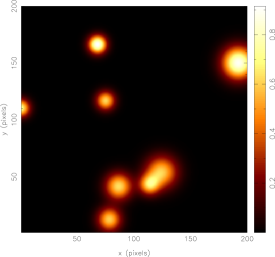
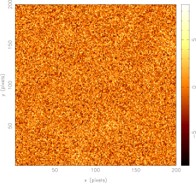
Figure 1: The toy problem discussed in section 4.3. The $200\times 200$ pixel test image (left panel) contains 8 discrete Gaussian-shaped objects of varying widths and amplitudes; the parameters $X_{k}$, $Y_{k}$, $A_{k}$ and $r_{k}$ for each object are listed in Table 1. The corresponding data map (right panel) has independent Gaussian pixel noise added with an rms of 2 units.

It is clear from the above that a crucial complication inherent to the problem of Bayesian object detection is that the length of the parameter vector $\mn@boldsymbol{\theta}$ is variable. In other words, the length of $\mn@boldsymbol{\theta}=\{N_{\rm obj},{\textbf{{a}}}_{1},{\textbf{{a}}}_{2},\ldots,{\textbf{{a}}}_{N_{\rm obj}}\}$ depends upon the value of $N_{\rm obj}$. Thus, in the MH algorithm, the proposal distribution must be able to propose moves between spaces of differing dimension. In this case, the detailed balance conditions must be carefully considered (Green 1994; Phillips & Smith 1995). The ability to sample from spaces of different dimensionality is incorporated in the Bayesys software.

4.3 A toy problem

In order to illustrate the various approaches to Bayesian object detection that we present below, we shall apply them to the simple toy problem illustrated in Fig. 1.

Object	$X$	$Y$	$A$	$R$
1	0.7	110.5	0.71	5.34
2	68.2	166.4	0.91	5.40
3	75.3	117.0	0.62	5.66
4	78.6	12.6	0.60	7.06
5	86.8	41.6	0.63	8.02
6	113.7	43.1	0.56	6.11
7	124.5	54.2	0.60	9.61
8	192.3	150.2	0.90	9.67

Table 1: The parameters $X_{k}$, $Y_{k}$ $A_{k}$ and $R_{k}$ $(k=1,\ldots,8)$ defining the Gaussian-shaped objects in Fig. 1. The objects are labelled in order of increasing $X$-value.

The left panel shows our $200\times 200$-pixel test image, which contains 8 Gaussian objects defined by (12); the parameters $X_{k}$, $Y_{k}$ $A_{k}$ and $R_{k}$ $(k=1,\ldots,8)$ are listed in Table 1 in order of increasing $X$-value. The $X$ and $Y$ position coordinates are drawn independently from the uniform distribution ${\cal U}(0,200)$ Similarly, the amplitude $A$ and size $R$ of each object are drawn independently from the uniform distributions ${\cal U}(0.5,1)$ and ${\cal U}(5,10)$ respectively. In the right panel of Fig 1, we plot the corresponding data map, which has independent (‘white’) Gaussian pixel noise added, with an rms of 2 units. This corresponds to a signal-to-noise ratio of 0.25–0.5 as compared to the peak emission in each object. We see from the figure that, with this level of noise, no objects are visible to the naked eye, and so this toy problem represents a considerable challenge for any object detection algorithm.

5 Simultaneous detection of all objects

The theoretically most desirable approach is to attempt to detect and characterise all the objects in the image simultaneously by sampling from the (unnormalised) posterior distribution (14), with the likelihood $\Pr({\textbf{{D}}}|\mn@boldsymbol{\theta})$ given by (15) and the prior $\Pr(\mn@boldsymbol{\theta})$ given by (16). Thus, this approach allows one to include prior information regarding the number of objects expected in the image. As mentioned above, however, in this case the length of the parameter vector $\mn@boldsymbol{\theta}$ is variable, which can lead algorithmic complications. Moreover, if the expected number of objects in the image is large, then so too will be the size of the corresponding parameter space that must be sampled. As a result, the algorithm can be slow to burn-in and requires a large amount of CPU time.

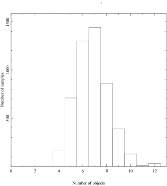
Figure 2: Left: histogram of the number of post burn-in samples obtained in each subspace corresponding to a different number of objects $N_{\rm obj}$. Right: the samples obtained for $N_{\rm obs}=7$, projected into the $(X,Y)$-subspace; the ellipses indicate the samples used in the calculation of the properties of the objects listed in Table. 2.

In the analysis of the toy problem discussed above, we assume the Poisson prior (17) on the number of objects $N_{\rm obj}$, with a mean of $\mu=4$, which is purposely chosen to be somewhat smaller than the actual number of objects $N_{\rm obj}=8$. Since the Poisson prior imposes no upper limit on the possible number of objects, the overall parameter space under consideration is formally the countably infinite union of subspaces

$$\Theta=\bigcup_{N_{\rm obj}=0}^{\infty}\Theta_{N_{\rm obj}},$$

where $\Theta_{N_{\rm obj}}=\{{\textbf{{a}}}_{1},\ldots,{\textbf{{a}}}_{N_{\rm obj}}\}$ denotes the $4N_{\rm obj}$-dimensional space corresponding to the model with $N_{\rm obj}$ objects. The parameters of the $k$th object are ${\textbf{{a}}}_{k}=\{X_{k},Y_{k},A_{k},R_{k}\}$, where we assume (correctly) that $X_{k}$ and $Y_{k}$ $(k=1,\ldots,N_{\rm obj})$ are drawn independently from the uniform distribution ${\cal U}(0,200)$. For $A_{k}$ and $R_{k}$, we again (correctly) assume that they are drawn independently from uniform distributions, but we overestimate the width of these distribuion. In particular, we assume $A_{k}$ and $R_{k}$ to be drawn from the uniform distributions ${\cal U}(0,2)$ and ${\cal U}(3,12)$ respectively.

In sampling from the parameter space, we used 10 Markov chains and took 5000 post burn-in samples. The results of this approach are illustrated in Fig. 2. In the left panel, we plot a histogram of the number of samples obtained in each subspace of different dimension, from which we note that the most favoured number of objects is $N_{\rm obj}=7$. One is free to use the 5000 post burn-in samples in a variety of ways to place limits on the parameters $\mn@boldsymbol{\theta}$. For illustration only, in the right panel of Fig. 2, we plot the samples obtained for the case $N_{\rm obs}=7$, projected into the $(X,Y)$-subspace. We see that there exist seven main areas in which the samples are concentrated, which we highlight with ellipses. Comparison with Fig. 1 (left panel) shows that each of these areas corresponds to a real object. The mean and standard deviation of the parameters $\{X_{k},Y_{k},A_{k},R_{k}\}$ $(k=1,\ldots,7)$ for each detected object were calculated from the samples contained in each ellipse. The results are given in Table 2, from which we see that the objects have been characterised to reasonable accuracy.

Object	$X$	$Y$	$A$	$R$
1	$4.6\pm 3.3$	$113.2\pm 3.4$	$0.90\pm 0.52$	$5.22\pm 2.60$
2	$65.8\pm 2.9$	$168.2\pm 2.0$	$0.97\pm 0.35$	$4.70\pm 1.27$
3	$74.7\pm 2.5$	$114.5\pm 2.8$	$0.88\pm 0.42$	$5.35\pm 1.95$
4	$76.4\pm 4.3$	$14.2\pm 5.0$	$0.69\pm 0.21$	$9.28\pm 2.14$
5	$88.6\pm 2.9$	$44.4\pm 3.7$	$0.63\pm 0.23$	$7.20\pm 1.76$
6 and 7	$120.3\pm 1.9$	$44.9\pm 1.9$	$0.93\pm 0.18$	$9.45\pm 1.25$
8	$188.7\pm 7.0$	$149.2\pm 1.7$	$1.22\pm 0.34$	$6.76\pm 2.41$

Table 2: The mean and standard deviation of the parameters $X_{k}$, $Y_{k}$ $A_{k}$ and $R_{k}$ $(k=1,\ldots,7)$ calculated from the samples contained within each ellipse in Fig. 2.

We must note, however, that the two overlapping objects 6 and 7 in Fig. 1 have been confused, and yield a single detected ‘object’. Moreover, for ‘objects’ 4 and 8, the samples in Fig. 2 (right panel) are not tightly concentrated into a single cluster at the true position of the object. Indeed, for ‘object’ 8, there is some indication that the samples are concentrated into two distinct regions, and may in fact represent two distinct objects, one of which is spurious.

Clearly there exist more optimal strategies for using the samples to characterise the objects and distinguish between real and spurious detections. Although we address these issues in the next section, in the context of iterative object detection, we shall not investigate further here. The reason for this is the rather computationally-intensive nature of the above approach. Using 10 chains and collecting 5000 samples after burn-in required $\sim 5\times 10^{6}$ evaluations of the posterior distribution. Since the noise is uncorrelated the noise covariance matrix N in the likelihood function (15) is diagonal, and so the posterior may be evaluated quickly. In 1 min of CPU time on an Intel Pentium III 1 GHz processor, the posterior distribution can be evaluated $\sim 5000$ times. Nonetheless, the total analysis required $\sim 17$ hrs of CPU time. As we discuss below, the process of object detection can be greatly simplified by adopting an iterative procedure, and so we shall not pursue the simultaneous detection algorithm further here.

6 Iterative object detection

An alternative approach to that discussed above, which is both algorithmically simpler and considerably computationally faster, is to replace the prior (17) by

$$\Pr{(N_{\rm obj})}=\left\{\begin{array}[]{ll}1&\mbox{if $N_{\rm obj}=1$}\\ 0&\mbox{otherwise}.\end{array}\right.$$

In other words, our model for the data consists of just a single object and so the full parameter space under consideration is simply ${\textbf{{a}}}=\{X,Y,A,R\}$, which is ‘only’ 4-dimensional. Although we have fixed $N_{\rm obj}=1$, it is important to understand that this does not restrict us to detecting just a single object in the data map. Indeed, by modelling the data in this way, we would expect the posterior distribution to possess numerous local maxima in the 4-dimensional parameter space, each corresponding to the location in this space of one of the objects.

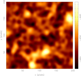
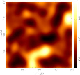
Figure 3: The 2-dimensional conditional log-posterior distributions in the $(X,Y)$-subspace for the toy problem illustrated in Fig. 1, where the model contains a single object parametrised by ${\textbf{{a}}}=\{X,Y,A,R\}$. The values of the amplitude $A$ and size $R$ are conditioned at $A=0.75$, $R=5$ (left panel) and $A=0.75$, $R=10$ (right panel).

This is best illustrated by direct evaluation of the posterior distribution. As mentioned in section 2, the ideal theoretical solution to any Bayesian inference problem is to calculate the full posterior distribution over some hypercube in parameter space that contains all the probability. However, even in the 4-dimensional parameter space we are considering here, this task is numerically intensive (indeed, this was the original motivation for using MCMC sampling techniques). Nevertheless, for the specific example at hand, the likelihood function (15) has a particularly simple form. It is thus computationally reasonable to calculate the full posterior distribution over some subspace of the 4-dimensional parameter space. It is most illustrative to calculate the posterior distribution in the 2-dimensional subspace defined by object position $(X,Y)$, while conditioning on particular values of $A$ and $R$.

In Fig. 3, we plot the 2-dimensional conditional log-posterior distribution in the $(X,Y)$-subspace for $A=0.75$, $R=5$ (left panel) and for $A=0.75$, $R=10$. The value $A$ is chosen to be the mean of the uniform distribution ${\cal U}(0.5,1)$ from which the amplitudes of the objects were drawn, whereas the two values of $R$ correspond to the limits of the uniform distribution ${\cal U}(5,10)$ from which the sizes of the objects were drawn. Each conditional log-posterior distribution is calculated on a $200\times 200$ grid in the $(X,Y)$-subspace, which requires around 10 mins of CPU time on an Intel Pentium III 1 GHz processor. We note that to calculate the full 4-dimensional log-posterior distribution at 200 points in each direction would require $200^{2}\times 10\mbox{ mins}\approx 280$ days of equivalent CPU time.

We see from Fig. 3 that the conditional log-posterior distributions contain multiple maxima and minima. As one might expect, maxima do occur at the positions corresponding to each of the 8 objects shown in Fig. 1. We also note, however, that the distributions contains numerous maxima that do not coincide with the position of a real object, but instead occur because the background noise in some areas has ‘conspired’ to give the impression that an object might be present. Unsurprisingly, this is particularly pronounced in the case $R=5$ (left panel). The effect is also easily seen in the $R=10$ case (right panel), but the distribution is correspondingly smoother, as one might expect. In either case, we see that pronounced peaks in the log-posterior occur only for objects 2, 4, 7 and 8 (as listed in Table 1). The peaks associated with the remaining objects are not distinguishable by eye from ‘false’ peaks in the log-posterior that occur at positions where no object is present. Finally, we note that for larger/smaller values of $A$ in the range $[0.5,1]$, the relative height of the peaks in the posterior distribution at positions of true objects increases/decreases slightly, but the overall shape of the distribution remains very similar.

6.1 Sampling of the posterior

It is clear from Fig. 3 that the full 4-dimensional posterior distribution will be very complicated, possessing multiple extrema. In particular, it is immediately obvious that any attempt to detect objects by straightforward maximisation (e.g. gradient search) of the posterior distribution is doomed to failure. We therefore choose instead to sample from the posterior using the MCMC approach outlined in section 3.

Several strategies present themselves for performing this sampling of the posterior. The conceptually most straightforward approach is to perform a ‘detailed’ sampling of the full 4-dimensional posterior. This may be achieved in the following way. Firstly, the use of several chains ($\sim$ the number of objects expected) allows the sampler to explore full parameter space more easily. Moreover, using a very slow annealing schedule and a correspondingly long burn-in period during the thermodynamic integration (see section 3.3), affords the chains greater opportunity to sample remote regions of the posterior distribution. Finally, after burn-in, a large number of samples are taken.

In general, however, the use of multiple chains, a long-burn and a large number of samples make this approach very time consuming, as was the case for the simultaneous detection of objects discussed in the previous section. This is particularly true, when the posterior distribution is dominated by a pronounced peak (or set of peaks) corresponding to one (or more) object. This can occur, for example, if the true amplitudes $A$ of some of the objects are much larger than the others, or simply by chance in cases where the signal-to-noise ratio is somewhat higher than that used in our toy problem. In this case, a significant fraction of the samples obtained are in the neighbourhood(s) of the pronounced peak(s), and so a large total number of samples are needed in order to obtain a reasonable representation of the full posterior distribution. We shall therefore not pursue the ‘detailed’ sampling approach here.

6.1.1 The McClean algorithm

The drawbacks associated with the above method do themselves, however, suggest an alternative iterative approach to the problem, in which one attempts to detect and characterise one (or a few) object at a time. In this case, one is not concerned with ‘detailed’ sampling of the full posterior distribution. Instead, one is content with sampling the distribution adequately in the neighbourhood of its most pronounced peak(s). This can be performed efficiently using only a few chains, a relatively fast annealing schedule during the thermodynamic integration, and requires many fewer post burn-in samples. Hence, this approach is significantly computationally faster than the ‘detailed’ sampling of the full posterior distribution. Having characterised the object(s) detected in this way, it (they) can then be subtracted from the data and the process repeated. In this way, the new log-posterior distribution will no longer contain the pronounced peak(s) associated with the subtracted object(s), but will instead be dominated by peaks associated with the most significant remaining object(s). This procedure has some features reminiscent of the widely-used Clean algorithm (Högbom 1974) for producing astronomical images from radio-inteferometer data. Since our approach is based on MCMC sampling techniques, we thus call it the McClean algorithm.

One remaining question is when to stop the iterative process. In fact, this may be answered straightforwardly using the notion of Bayesian evidence, discussed in section 2.2. Let us denote the model (hypothesis) that there are no objects (remaining) in the image by $H_{0}$, and the model consisting of a single (remaining) object, i.e. $N_{\rm obj}=1$, by $H_{1}$. Since $H_{0}$ has no parameters associated with it, the evidence $\Pr({\textbf{{D}}}|H_{0})$ is simply the value of the likelihood function (15) evaluated for the case with no objects in the data. The model $H_{1}$, however, depends on the parameters ${\textbf{{a}}}=\{X,Y,A,R\}$, and the evidence is given by

$$\Pr({\textbf{{D}}}|H_{1})=\int\Pr({\textbf{{D}}}|{\textbf{{a}}})\Pr({\textbf{{a}}})\,d{\textbf{{a}}}.$$

As shown in section 2.2, the value of the evidence $\Pr(D|H_{1})$ may be evaluated (to a good approximation) from the MCMC samples using thermodynamic integration. Thus, after each iteration of the McClean algorithm, one calculates the evidence ratio $\Pr({\textbf{{D}}}|H_{1})/\Pr({\textbf{{D}}}|H_{0})$. If this ratio is greater than unity one accepts the identified object(s) and repeats the procedure. If the ratio is less than unity, the object(s) identified in the last iteration are discarded, and the algorithm is stopped.

From its design, it is clear that the McClean algorithm is a compromise between the full Bayesian approach outlined in section 5 and the desire to obtain results in a reasonable amount of CPU time. For the toy problem at hand, it is clearly a sensible approach, which we show below yields good results. As an approximation to the fully Bayesian method, however, there will inevitably be situations in which its performance is poorer. A discussion of straightforward refinements to the basic McClean algorithm, which broaden its range of applicability, while retaining its computational efficiency, are given in section 8.

6.1.2 Application to the toy problem

We now apply the McClean algorithm to the toy problem discussed in section 4.3 and illustrated in Figs 1 and 3.

Figure 4: The 500 samples from the posterior obtained on the third iteration of the McClean algorithm when applied to the toy problem. The samples are projected into the 2-dimensional subspaces $(X,Y)$ (left panel) and $(A,R)$ (right panel).

We perform the MCMC sampling using 5 chains and, at each iteration, 500 post burn-in samples are taken from the posterior, and the algorithm identifies 6 objects before stopping. The total analysis required $\sim 2\times 10^{5}$ evaluations of the posterior, which took $\sim 40$ mins of CPU time on a single Intel Pentium III 1 GHz processor; this is clearer considerably less computationally intensive than attempting to detect all the objects simulaneous, as discussed in section 5.

The detected objects are listed in Table 3 in the order in which they are identified. For each identified object, the table also lists the mean and standard deviation of the 1-dimensional marginalised distribution for each parameter $\{X,Y,A,R\}$.

Object	$X$aaaa	$Y$aaaa	$A$aaaa	$R$ aaaa
8	$192.6\pm 2.5$	$149.0\pm 2.0$	$0.93\pm 0.17$	$9.47\pm 1.33$
6 and 7	$118.3\pm 2.3$	$50.5\pm 1.9$	$0.90\pm 0.24$	$8.32\pm 1.65$
4	$79.0\pm 1.9$	$12.2\pm 2.2$	$1.04\pm 0.26$	$7.08\pm 1.57$
5	$86.6\pm 3.2$	$40.5\pm 2.5$	$0.63\pm 0.19$	$8.10\pm 1.61$
2	$64.9\pm 2.4$	$164.0\pm 2.3$	$0.74\pm 0.32$	$5.94\pm 1.51$
1	$4.2\pm 2.9$	$108.7\pm 3.1$	$0.61\pm 0.27$	$6.41\pm 1.92$

Table 3: The objects identified by the McClean algorithm when applied to the toy problem discussed in section 4.3. The objects are listed in the order in which they were identified. The mean and standard deviation of the 1-dimensional marginalised distributions for each parameter $\{X,Y,A,R\}$ are listed for each identifed object.

Comparing these values with those listed in Table 1, we see that the algorithm has accurately recovered the true parameter values for objects 8,4,5,2 and 1, within the stated errors. The second identified ‘object’ listed in Table 3 is, however, a composite of the two real overlapping objects 6 and 7, which the algorithm has been unable to separate with the applied level of pixel noise. The algorithm also fails to identify object 3. In fact, if the algorithm is allowed to continue past the point where the evidence criterion suggests termination, one finds that some samples from the posterior are clustered in the neighbourhood of object 3. However, samples in these later iterations are also clustered in other areas where no real objects are located, but maxima nevertheless exist in the posterior (as illustrated in Fig. 3). Thus, the evidence-based stopping criterion provides a robust method for avoiding spurious detections.

For each identified object, the samples from the posterior clearly contain more information than simply the mean and standard deviation of its defining parameters. As an illustration, in Fig. 4 we plot the 500 samples obtained on the third iteration of the algorithm (which identified object 4) projected into the two 2-dimensional subspaces $(X,Y)$ and $(A,R)$. By projecting these samples further into 1-dimensional subspaces, we obtain four marginalised distributions for the parameters $X$, $Y$, $A$ and $R$ separately; these are shown in Fig. 5.

Figure 5: The 500 samples from the posterior obtained on the third iteration of the McClean algorithm, projected into 1-dimensional subspaces to yield the marginalised distributions for the parameters $X$, $Y$, $A$ and $R$ separately.

The number of objects detected by the algorithm, and the accuracy with which their defining parameters are determined, will clearly depend on the rms level of the added pixel noise. For comparison, in Table 4, we list the objects detected for the case where the rms noise level is increased to 3 units. This noise level corresponds to a signal-to-noise ratio of $0.16-0.33$ as compared with the peak values of the objects.

Object	$X$aaaa	$Y$aaaa	$A$aaaa	$R$ aaaa
4	$79.1\pm 1.8$	$11.1\pm 2.6$	$1.19\pm 0.30$	$6.95\pm 1.33$
8	$192.5\pm 3.1$	$149.5\pm 2.6$	$1.04\pm 0.31$	$8.73\pm 1.95$
6 and 7	$118.4\pm 2.5$	$51.2\pm 2.0$	$1.21\pm 0.39$	$6.40\pm 1.90$
5	$85.6\pm 7.1$	$39.1\pm 5.6$	$0.58\pm 0.32$	$8.10\pm 2.46$

Table 4: As in Table 3, but for an rms noise level of 3 units.

We see that, in the presence of a noise background with a larger rms, the algorithm detects only 4 distinct objects, with the real objects 6 and 7 again combined into a single detection. Nevertheless, the defining parameters of those object identified are once again accurate to within the derived errors.

It is also of interest to consider lower noise levels. In Table 5, we list the objects detected in the case for which the rms noise level is decreased to 1 unit, which corresponds to a signal-to-noise ratio of $0.5-1$ as compared with the peak values of the objects.

Object	$X$aaaa	$Y$aaaa	$A$aaaa	$R$ aaaa
8	$192.3\pm 1.3$	$149.7\pm 1.0$	$0.90\pm 0.08$	$9.70\pm 0.83$
6 and 7	$118.6\pm 1.3$	$50.1\pm 1.1$	$0.72\pm 0.09$	$9.7\pm 0.89$
4	$79.0\pm 1.0$	$12.6\pm 1.2$	$0.79\pm 0.13$	$7.24\pm 0.99$
5	$86.2\pm 1.3$	$40.8\pm 1.2$	$0.63\pm 0.10$	$7.81\pm 0.79$
2	$66.6\pm 1.0$	$165.1\pm 0.85$	$0.93\pm 0.19$	$4.99\pm 0.74$
3	$73.8\pm 1.5$	$116.1\pm 1.5$	$0.64\pm 0.15$	$5.22\pm 0.79$
1	$2.4\pm 1.1$	$109.0\pm 1.57$	$0.67\pm 0.18$	$5.85\pm 1.32$

Table 5: As in Table 3, but for an rms noise level of 1 unit.

In this case, we see that the algorithm detects all the real objects with high accuracy, except for once again combining the overlapping objects 6 and 7 into a single detection. Indeed, this degeneracy can only be broken when the rms noise level falls below $\sim 0.5$ units. This is easily understood if one plots the conditional log-posterior in the $(X,Y)$-subspace (i.e. analogous to Fig 3) for some typical values of $A$ and $R$ and for various noise levels. Only for $\sigma\la 0.5$ units does the log-posterior distribution in the location of objects 6 and 7 divide into two distinct maximia. In this case, as one would expect, the algorithm identifies objects 6 and 7 as separate features, and finds the correct defining parameters for each object within the derived errors. It is worth noting in Tables 3 & 5 that the recovered $X$-position for object 1 is slightly less accurate than for the other objects, since it is located at the edge of the observed field.

6.2 Global maximisation of the posterior

Instead of sampling from the posterior using MCMC techniques, one can obtain a less theoretically-desirable, but much faster, solution by simply locating the global maximum of the posterior at each iteration. The price to be paid for dispensing with the sampling approach is that one must return to the more traditional method, outlined in section 2, of characterising the posterior distribution in terms of a set of best estimates $\hat{{\textbf{{a}}}}=\{\hat{X},\hat{Y},\hat{A},\hat{R}\}$ that locate its global maximum. Similarly, one must be content with describing the uncertainties in the derived parameters in terms of the estimated covariance matrix given by (minus) the inverse of the Hessian matrix at the global maximum. Nevertheless, this approach is perfectly adequate for most applications.

6.2.1 The MaxClean algorithm

It is clear from the conditional log-posterior distributions for the toy problem, shown in Fig. 3, that a numerical maximiser (minimiser) which locates only a local maximum will most often produce a spurious detection. One must instead seek to locate the global maximum of the posterior. In fact, an MCMC sampler can itself be used to locate the global maximum in parameter space. This is most easily achieved by introducing an annealing parameter similar to that used in thermodynamic integration (see section 3.3). In this case, however, one raises the full (unnormalised) posterior $\overline{\Pr}(\mn@boldsymbol{\theta}|{\textbf{{D}}})$ to the power $\lambda$. Allowing this parameter to continue increasing gradually beyond unity artificially ‘sharpens’ the posterior distribution. As $\lambda$ grows the samples are then concentrated into an increasingly compact region of parameter space, and eventually locate the global maximum to some required accuracy. Nevertheless, even if one does not have access to a reliable MCMC sampler, one may still perform Bayesian object detection and characterisation using elementary and widely-available algorithms, as we illustrate below.

The most widely-used technique for performing locating a global extremum is simulated annealing. In particular, we use the downhill simplex implementation of a simulated annealing minimiser suggested by Press et al. (1994). In short, this algorithm behaves in the same way as a standard downhill simplex minimiser, except that one adds a positive, logarithmically-distributed random variable, proportional to the annealing temperature $T$, to the function value associated with each vertex of the simplex. Then a similar random variable is subtracted from the function value of every new point that is tried as a replacement vertex. In this way, the algorithm always accepts a true downhill step, but sometimes accepts an uphill one. Indeed, for a finite $T$-value, the algorithm can wander freely among local minima of depth less than about $T$. As $T$ is reduced according to some annealing schedule, the number of minima qualifying for frequent visits is reduced and, in the limit $T\to 0$, the algorithm reduces exactly to the standard downhill simplex minimisation method and converges to the nearest local minimum. If the annealing schedule reduces the temperature $T$ sufficiently slowly, it is very likely that the simplex will shrink into the region containing the global minimum.

Possible choices for the annealing schedule are discussed by Press et al. (1994). We found that an effective approach was simply to reduce $T$ from some initial starting value $T_{0}$ by a fixed factor $f$, after every $N_{\rm iter}$ moves of the simplex vertices. The choice of $T_{0}$, $f$ and $N_{\rm iter}$ are problem-specific, and are discussed below with reference to the toy problem.

Once one has a technique for reliably locating the global maximum of the posterior distribution, the basic iterative procedure for object detection is analogous to the McClean algorithm discussed above. In this case, however, only one object can be identified and removed in each iteration. We call the resulting procedure the MaxClean algorithm.

Finally, one must reconsider the problem of when to stop the algorithm. Ideally, one would like to use the evidence ratio $\Pr({\textbf{{D}}}|H_{1})/\Pr({\textbf{{D}}}|H_{0})$ as our stopping criterion, as discussed above for the McClean algorithm. Once again $\Pr({\textbf{{D}}}|H_{0})$ is simply the value of the likelihood function evaluated for the model containing no objects. In the absence of samples from the posterior, however, one cannot obtain the evidence $\Pr({\textbf{{D}}}|H_{1})$ for the single-object model by performing a thermodynamic integration. Nevertheless, an approximate value for the evidence $\Pr({\textbf{{D}}}|H_{1})$ after each iteration can be obtained by approximaing the posterior distribution as a 4-dimensional multivariate Gaussian about the corresponding global maximum found by the simulated annealing simplex algorithm. As discussed in section 2.2, an approximate value for the evidence is then given by (8). The covariance matrix C appearing in this expression is simply (minus) the inverse of the Hessian matrix of the log-posterior at the peak. In turn, we find that a good approximation to this Hessian matrix is obtained by using simple second-differencing algorithm along each parameter direction. Hence, the Gaussian approximation to the evidence $\Pr({\textbf{{D}}}|H_{1})$ may be easily and quickly calculated, and the resulting (approximate) evidence ratio can be used to determine when to halt the algorithm.

6.2.2 Application to the toy problem

We now apply the MaxClean algorithm to the toy problem discussed in section 4.3 and illustrated in Figs 1 & 3, for the case in which the rms of the pixel noise is 2 units. As mentioned above, in order to apply the MaxClean algorithm one must first define an effective annealing schedule. We find that a robust approach is as follows: starting from some initial annealing temperature $T_{0}$, after every $N_{\rm iter}$ moves of the simplex vertices one reduces $T$ by a fixed factor $f$. The choice of $T_{0}$, $f$ and $N_{\rm iter}$ clearly affects the total required number of evaluations of the posterior distribution, and hence the overall speed of the algorithm. This choice also affects the efficiency with which the global maximum can be located.

Figure 6: The position of the ‘best-point’ in the simplex after each move, during the third iteration of the MaxClean algorithm (in which object 4 is detected). Each point is plotted simultaneously in the $(X,Y)$ and $(A,R)$-subspaces. The position to which the simplex converged is indicated by the short arrows.

As stated above, for a finite value of $T$, the simplex can wander freely among local maxima (minima) of height less than about $T$. Thus one must set $T_{0}$ to be at least of the order of the largest variations one expects in the log-posterior distribution. From Fig. 3, we see that log-posterior varies by $\sim 70$ units in the $(X,Y)$-subspace corresponding to the conditioned values $A=0.75$, $R=5$ and $A=0.75$, $R=10$. In order that the simplex has access to all regions of the log-posterior in the early stages of the annealing schedule, we thus set $T_{0}=100$. We note that, in the absence of this prior information one could set $T_{0}$ to some arbitrarily large value, but at the cost of requiring a larger total number of function evaluations before the algorithm converges. In choosing the fixed factor $f$, one must ensure that the annealing schedule reduces the temperature ‘slowly enough’ that the algorithm converges to the global maximum of the log-posterior. We find that the convergence of the algorithm is reasonably insensitive to the precise value of $f$, provided it lies in the range $1\la f\la 4$; we choose $f=1.5$ for the results presented below. Finally, the parameter $N_{\rm iter}$ determines the number of moves of the downhill simplex performed at each value of the annealing temperature $T$ (until convergence is obtained). We again find the convergence of the algorithm to the global maximum is reasonably insensitive to this parameter, provided $N_{\rm iter}\ga 50$; we choose $N_{\rm iter}=200$ for the results presented below.

We find that the MaxClean algorithm works very well on the toy problem and produces results similar to those presented in section 6.1.2, obtained using McClean.

Object	$X$aaaa	$Y$aaaa	$A$aaaa	$R$ aaaa
8	$191.3\pm 2.5$	$149.5\pm 2.1$	$0.99\pm 0.10$	$8.59\pm 0.69$
6 and 7	$118.8\pm 1.9$	$51.0\pm 1.8$	$0.99\pm 0.24$	$7.64\pm 0.67$
4	$78.6\pm 1.5$	$11.8\pm 1.7$	$1.10\pm 0.17$	$6.51\pm 0.98$
5	$86.8\pm 3.6$	$40.3\pm 2.5$	$0.64\pm 0.12$	$8.38\pm 1.40$
2	$64.9\pm 2.3$	$164.1\pm 2.0$	$0.86\pm 0.34$	$5.36\pm 2.62$
1	$0.2\pm 5.1$	$108.3\pm 2.8$	$0.92\pm 0.24$	$6.47\pm 1.65$

Table 6: The objects identified by the MaxClean algorithm when applied to the toy problem discussed in section 4.3. The objects are listed in the order in which they were identified. The derived parameters correspond to the global maximum of the posterior distribution at each iteration of the algorithm. The quoted errors on the parameters of each object refer to the square-root of the corresponding diagonal element of the covariance matrix derived from the Hessian at the peak.

The objects identified are listed in Table 6. We note that the order in which they are detected by the MaxClean algorithm is the same as that produced by McClean. Indeed, one would expect this to be the case, since at each iteration each algorithm either samples the posterior in the neighbourhood of the global maximum or locates its position directly. We also see from Table 6 that the parameters defining the identified objects are in reasonable agreement with the true values listed in Table 1 and are similar to those obtained using the McClean algorithm, listed in Table 3. It must be remembered, however, that, for each object, the derived parameter values and estimated errors produced by the McClean and MaxClean algorithms are defined in different ways. In McClean they correspond respectively to the mean and 68-per cent confidence limits of the 1-dimensional marginalised distribution for each parameter as derived from the MCMC samples. In MaxClean, however, the estimated parameter values correspond simply to the location of the global maximum of the multi-dimensional posterior and the errors are approximated by the square-root of the appropriate diagonal element of the covariance matrix, derived from the Hessian at the peak. We also note in Table 6 that the quoted error on the recovered $X$-position of object 1 is larger that for the other objects, since it lies at the edge of the observed field.

In Fig. 6, we plot an illustration of the behaviour of the simulated-annealing downhill simplex miminiser on the third iteration of the MaxClean algorithm (in which object 4 is detected). Since the parameter space is 4-dimensional, the simplex has 5 vertices. For each move of the simplex, we plot the position of the vertex corresponding to the largest value of the posterior distribution in the $(X,Y)$ and $(A,R)$-subspaces; the position to which the simplex eventually converged is indicated by the arrows. After exploring the log-posterior distribution for a few iterations, the simplex vertices are concentrated in the neighbourhood of the global maximum. As the annealing temperature is reduced the algorithm convergences ever more tightly on the position of the peak.

With the choice of annealing schedule parameters $T_{0}$, $f$ and $N_{\rm iter}$ discussed above, the detection of all the objects listed in Table 6 required $\sim 40000$ evaluations of the log-posterior. The entire analysis was completed in $\sim 8$ mins on a Pentium III 1 GHz processor, which is somewhat faster the McClean algortihm, as might be expected. Finally, we note also that the MaxClean algorithm also obtains similar results to those produces by McClean algorithm for the case in which the rms of the pixel noise is decreased to 1 unit or increased to 3 units (see section 6.1.2).

7 Detecting the SZ effect in CMB maps

As a cosmological illustration of the Bayesian approach to detecting discrete objects in a background, in this section we consider the specific problem of identifying the Sunyaev-Zel’dovich (SZ) effect from clusters embedded in maps of emission due to primordial cosmic microwave background (CMB) anisotropies. The dominant microwave emission from clusters of galaxies is the thermal SZ effect, in which CMB photons are inverse Compton scattered to higher energies by fast moving electrons in the hot intracluster gas. This leads to a characteristic frequency dependence for the thermal SZ effect that differs markedly from that of the primordial CMB emission. The kinetic SZ effect is due to the Doppler effect from clusters with a peculiar velocity along the line of sight, and thus has the same frequency behaviour as the primordial CMB emission. Moreover, the kinetic SZ effect is typically an order of magnitude smaller than the thermal effect. A recent review of both the thermal and kinetic SZ effects is given by Zhang, Pen & Wang (2002).

The important problem of detecting SZ clusters in microwave maps dominated by primordial CMB emission has been considered previously by several authors, and most recently by Herranz et al. (2002a,b), who considered the thermal SZ effect. In these recent analyses, the identification and characterisation of thermal SZ clusters were performed using the scale-adaptive linear filtering technique developed by Sanz et al. (2001). In the former, only maps at a single observing frequency were considered, whereas in the latter the different spectral dependences of the SZ and CMB emission were also used to differentiate between the two (and other) components.

The Bayesian approach to object detection outlined in the previous sections (using either the McClean or MaxClean algorithms) can be applied straightforwardly to either single or multi-frequency data. In this section, however, we will concentrate on the analysis of a single-frequency map. The Bayesian analysis of detailed simulated multi-frequency SZ and CMB observations will be presented in a forthcoming paper.

7.1 The thermal SZ effect

Let us first consider the detection of the thermal SZ effect in clusters. Since our aim is merely to illustrate our Bayesian approach, we shall analyse a simple set of simulated observations, at a single observing frequency, using the McClean algorithm. The simulations assume each SZ cluster to be spherically-symmetric with an electron density profile of the form

$$n_{\em e}(r)=n_{0}\left[1+\left(\frac{r}{r_{c}}\right)^{2}\right]^{-3\beta/2}.$$

In this case, one easily finds that the projected thermal SZ profile on the sky, for a cluster centred at the position ${\textbf{{X}}}=(X,Y)$ with a central SZ amplitude $A$, is given by

$$\tau({\textbf{{x}}};X,Y,A,r_{c})=A\left(1+\frac{|{\textbf{{x}}}-{\textbf{{X}}}|^{2}}{r_{c}^{2}}\right)^{-\lambda}.$$ (18)

where $\lambda=(3\beta-1)/2$. Assuming the standard value $\beta=2/3$ gives $\lambda=1/2$. In this case, $\tau({\textbf{{x}}})$ has the rather unpleasant feature of possessing an infinite volume, and so its Fourier transform is singular at the origin of k-space. As advocated by Herranz et al. (2002a), however, this troublesome behaviour can be circumvented by replacing (18), for the case $\lambda=1/2$, by the modified profile

$$\tau({\textbf{{x}}};X,Y,A,r_{c})=\frac{Ar_{c}r_{v}}{r_{v}-r_{c}}\left(\frac{1}{\sqrt{r_{c}^{2}+d^{2}}}-\frac{1}{\sqrt{r_{v}^{2}+d^{2}}}\right),$$ (19)

where $d=|{\textbf{{x}}}-{\textbf{{X}}}|$ and $r_{v}$ may be interpreted as some typical ‘virial’ radius for the cluster; we set $r_{v}=3r_{c}$. The profile (19) has a finite volume and a non-singular Fourier transform.

Our simulations are performed at an observing frequency of 100 GHz on a $200\times 200$ grid, with a cell size of 1.5 arcmin, so that the simulated sky area is $5^{\circ}\times 5^{\circ}$. At 100 GHz, the dominant sky emission is due to primordial anisotropies in the CMB and we may reasonably neglect contaminating emission from the Galaxy. The CMB emission in our simulations is modelled by a homogeneous Gaussian random field with a standard inflationary cold dark matter power spectrum $C_{\ell}$. The assumed cosmological model is spatially flat with $\Omega_{\rm b}=0.05$, $\Omega_{\rm cdm}=0.3$ and $\Omega_{\Lambda}=0.65$. We also assume a reduced Hubble parameter $h=0.65$, a primordial scalar spectral index $n=1$, and no tensor modes. The $C_{\ell}$ coefficients were created using Cmbfast (Seljak & Zaldarriaga 1996). The rms of the CMB emission is $\sim$ 100 $\mu$K.

To model the thermal SZ emission from clusters, we uniformly distribute 15 profiles of the form (19) within the $5^{\circ}\times 5^{\circ}$ patch of sky. At 100 GHz, the thermal SZ effect produces a decrement, and so we draw the central amplitude $A$ (in $\mu$K) of each profile from the uniform distribution ${\cal U}(-500,-50)$. This corresponds SZ Compton $y$-parameters in the range $\sim 10^{-4}-10^{-5}$, which is typical for more realistic SZ simulations. The core radius $r_{c}$ (in arcmin) of each cluster is drawn from the uniform distribution ${\cal U}(0.75,3)$.

We include some experimental realism into our simulations by performing simulated observations that correspond to those expected from the forthcoming Planck mission. At 100 GHz, we model the Planck observing beam as a Gaussian with a FHWM of 10 arcmin, and we assume Gaussian instrumental pixel noise which is homogeneous and uncorrelated and has an rms of 20 $\mu$K. This noise level might reasonably be expected for the HFI 100 GHz channel after 24 months of obervation by Planck. After convolution with the beam, the central SZ amplitudes are considerably reduced and lie in the range $-130$ to $-10$ $\mu$K. Comparing these amplitudes with the total rms of the convolved CMB emission and the instrumental noise, the signal-to-noise ratio varies from 1.5 to 0.1, and this therefore presents a considerably challenging object detection problem. Fig. 7 shows the true thermal SZ emission in the simulations (left panel) and the convolved noisy data, which is clearly dominated by primordial CMB emission (right panel).

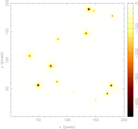
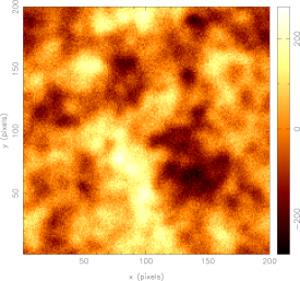
Figure 7: Left: the 15 thermal SZ modified King profiles used in our $5^{\circ}\times 5^{\circ}$ simulation (see text for details). Right: simulated Planck data of the same $5^{\circ}\times 5^{\circ}$ field at 100 GHz, assuming a Gaussian observing beam with a FWHM of 10 arcmin. In addition to the convolved thermal SZ signal, the map contains primordial CMB emission and instrumental noise (see text for details). Both maps are plotted in units of $\mu$K.

7.1.1 Evaluation of the posterior distribution

In order to perform the Bayesian object detection (using either McClean or MaxClean), one needs to calculate the posterior distribution a large number of times, each at a different point in the parameter space ${\textbf{{a}}}=\{X,Y,A,r_{c}\}$. Although the calculation of the priors is trivial, the evaluation of the likelihood function is computationally more demanding. Since the background ‘noise’ n (which consists of primordial CMB and instrumental pixel noise) is a Gaussian random field, the likelihood function has the form discussed in section 4, namely

$$\Pr({\textbf{{D}}}|{\textbf{{a}}})=\frac{\exp\left\{-{[{\textbf{{D}}}-{\textbf{{s}}}({\textbf{{a}}})]}^{\rm t}{\textbf{{N}}}^{-1}[{\textbf{{D}}}-{\textbf{{s}}}({\textbf{{a}}})]\right\}}{(2\pi)^{N_{\rm pix}/2}|{\textbf{{N}}}|^{1/2}}.$$ (20)

Unlike the toy problem discussed in section 4.3, however, the presence of the correlated CMB emission means that the ‘noise’ covariance matrix N is not diagonal. Since its dimensions are $N_{\rm pix}\times N_{\rm pix}$ (i.e. $200^{2}\times 200^{2}$ for our simulations), the direct calculation of the quadratic form and the determinant in (20) would be an extreme computational burden. Moreover, even the calculation of the signal ${\textbf{{s}}}({\textbf{{a}}})$ resulting from a source characterised by a given set of parameters a, would require one to perform a beam convolution for each likelihood evaluation. In general this requires requires two Fast Fourier Transforms (FFTs), which are themselves computationally intensive.

Fortunately, for the problem at hand, there exists a straightforward solution to these computational difficulties, which is simply to perform the entire calculation in Fourier space. Thus, we instead consider our data to be the Fourier transform $\widetilde{{\textbf{{D}}}}$ of our original data map. Then, since the background ‘noise’ is a homogeneous Gaussian random field, the likelihood function now takes the form

$$\Pr(\widetilde{{\textbf{{D}}}}|{\textbf{{a}}})=\frac{\exp\left\{-{[\widetilde{{\textbf{{D}}}}-\widetilde{{\textbf{{s}}}}({\textbf{{a}}})]}^{\dagger}\widetilde{{\textbf{{N}}}}^{-1}[\widetilde{{\textbf{{D}}}}-\widetilde{{\textbf{{s}}}}({\textbf{{a}}})]\right\}}{(\pi)^{N_{\rm pix}}|\widetilde{{\textbf{{N}}}}|},$$ (21)

where we note that several factors of two differ from the expression (20), since (21) is a multivariate Gaussian distribution of complex variables (Eaton 1983). In this expression, since the ‘noise’ background is a homogeneous random field, the ‘noise’ covariance matrix $\widetilde{{\textbf{{N}}}}$ is diagonal. Indeed, if we denote the Fourier transform of the observing beam by $\widetilde{B}(k)$, and the power spectra of the primordial CMB and instrumentional noise by $P_{\rm cmb}(k)$ and $P_{\rm n}(k)$ respectively, then

$$\widetilde{N}_{ij}=\langle\widetilde{n}({\textbf{{k}}}_{i})\widetilde{n}^{\ast}({\textbf{{k}}}_{j})\rangle=\left[|\widetilde{B}(k_{i})|^{2}P_{\rm cmb}(k_{i})+P_{\rm n}(k_{i})\right]\delta_{ij},$$ (22)

where $k=|{\textbf{{k}}}|$. For the case of a Gaussian observing beam with dispersion $\sigma_{b}$, the beam Fourier transform has the form $\widetilde{B}(k)=\exp(-\sigma_{b}^{2}k^{2}/2)$.

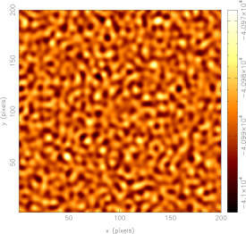
Figure 8: The 2-dimensional conditional log-posterior distributions in the $(X,Y)$-subspace for the thermal SZ detection problem illustrated in Fig. 7. The values of the central SZ amplitude and core radius are conditioned at $A=-250$ $\mu$K and $r_{c}=1.5$ arcmin.

Figure 9: Comparison of the true and estimated values of the parameters $X$, $Y$, $A$ and $r_{c}$ for the 7 thermal SZ clusters identified by the McClean algorithm (filled circles). The error bars on the estimated values denote the 68 per cent confidence limits of the corresponding marginalised posterior distribution. The 8 unidentified clusters are represented by the open squares plotted along the bottom of each graph.

The only remaining task in evaluating (21) is to calculate the signal $\widetilde{{\textbf{{s}}}}({\textbf{{a}}})$ resulting from a discrete object of the form (19), characterised by a given set of parameters ${\textbf{{a}}}=\{X,Y,A,r_{c}\}$. Fortunately, the two-dimensional Fourier transform of (19) is easily calculated to be

$$\widetilde{\tau}({\textbf{{k}}};X,Y,A,r_{c})=A\exp(-i{\textbf{{k}}}\cdot{\textbf{{X}}})\widetilde{\tau}(k;0,0,1,r_{c}),$$ (23)

where ${\textbf{{X}}}=(X,Y)$ and the Fourier transform $\widetilde{\tau}(k;0,0,1,r_{c})$ of the ‘standard object’ is given by

$$\widetilde{\tau}(k;0,0,1,r_{c})=\frac{2\pi r_{v}r_{c}}{r_{v}-r_{c}}\frac{\exp(-r_{c}k)-\exp(-r_{v}k)}{k}.$$ (24)

Despite appearances to the contrary $\widetilde{\tau}(k;0,0,1,r_{c})$ is well-defined at the origin of Fourier space, as is easily seen by evaluating the limit $k\to 0$. The signal $\widetilde{s}({\textbf{{a}}})$ in the data produced by an object with a particular parameterisation is then obtained by simply multiplying (23) by the beam Fourier transform $\widetilde{B}(k)$.

Thus, using (22)–(24), we may calculate the likelihood function (21) at minimal computational cost, entirely in Fourier space. Since we are assuming uniform priors on each of the parameters $\{X,Y,A,r_{c}\}$, the evaluation of the posterior distribution at any point in parameter space is also straightforward. To illustrate the structure of this function, in Fig. 8 we plot the 2-dimensional conditional log-posterior distribution in the $(X,Y)$-subspace corresponding to the simulated data shown in Fig. 7; in this plot the values of $A$ and $r_{c}$ are conditioned at $A=-250$ $\mu$K and $r_{c}=1.5$ arcmin (i.e. 1 pixel). We see that faint local maxima do indeed occur at the positions of the true SZ clusters, although these peaks are not greatly pronounced with respect to ‘chance’ fluctuations in the log-posterior caused by the CMB emission and the instrumental noise. This problem therefore represents a severe challenge for any object detection algorithm.

7.1.2 Application of the McClean algorithm

We now attempt to recover the SZ cluster profiles in the simulated data using the McClean algorithm discussed in section 6.1.1, which identifies objects iteratively by MCMC sampling from the full 4-dimensional posterior distribution. As in the toy problem, we use 5 Markov chains in the sampling process, and take 500 post burn-in samples from the posterior at each iteration.

The algorithm identifies 7 of the 15 objects present, before terminating when the evidence for a further object falls below that for the model containing no objects. The results are summarised in Fig. 9, in which the 7 identified clusters are denoted by the solid circles, and the open squares represent the 8 unidentified clusters. We see that the positions of the identified clusters are very accurately constrained. Indeed the error-bars plotted on the points are not visible. The typical error in $X$ or $Y$ is $\sim 0.75$ arcmin (i.e. $\sim 0.5$ pixels). The amplitude $A$ and core radius $r_{c}$ of each identified cluster are also recovered to reasonable accuracy, with the scatter about the true values well-described by the derived error-bars. As one might expect, the 7 clusters identified by the algorithm are those with the largest central SZ decrements, except for one cluster with $A=-355$ $\mu$K and $r_{c}=1.1$. This cluster is not detected since, owing to its small core radius, the central amplitude of this cluster is considerably reduced by the beam convolution. We note in particular that there are no spurious detections. The entire analysis required around $2.5\times 10^{5}$ function evaluations and took $\sim 50$ mins of CPU time on a Pentium III 1 GHz processor.

The above results assume an instrumental pixel noise rms of 20 $\mu$K, which corresponds to around 24 months of observation for the Planck HFI 100 GHz channel. It is expected, however, that preliminary Planck channel maps will be available after just 6 months of observation. For the HFI 100 GHz channel, the rms of the instrumental pixel noise on such a map will thus be about $\sqrt{4}\times 20=40$ $\mu$K. Since it is hoped that a preliminary catalogue of SZ clusters might be produced from these data, we have therefore repeated our analysis for this higher noise level. In this case, we find that the McClean algorithm identifies the same first five clusters that it found in the lower noise simulation, but then terminates. Despite detecting fewer clusters, we find that the typical errors on the position, amplitude and core radius of each identified cluster are very similar to those obtained for the lower noise case, and so are not plotted here.

7.1.3 Comparison with linear filter techniques

It is worthwhile to compare the performance of the McClean algorithm with more traditional filtering techniques, such as those proposed by Herranz et al. (2002a). In order to make a direct comparison, we now apply the McClean algorithm to an alternative simulated dataset, which has the same statistical properties as ‘simulation 2’ in Herranz et al.

Our simulation again consists of a $5^{\circ}\times 5^{\circ}$ patch of sky, containing $200\times 200$ pixels of size 1.5 arcmin. The thermal SZ emission is modelled with the same 15 modified King profile clusters as shown in Fig. 7 (left panel). As discussed earlier, the central amplitudes of these SZ clusters are drawn from a uniform distribution covering one order of magnitude in temperature and their core radii are drawn uniformly between 0.75 and 3 arcmin. Indeed, this is precisely the statistical content of the SZ signal assumed in ‘simulation 2’ by Herranz et al. The only difference between the two simulations is the size of the patch of sky. In ‘simulation 2’, a $12^{\circ}.8\times 12^{\circ}.8$ patch of sky was considered, consisting of $512\times 512$ pixels, in which 100 such SZ clusters were randomly distributed. Clearly, the two simulations share the same pixel size and the same average number of clusters per deg². Following ‘simulation 2’, we add to the SZ clusters a ‘CMB’ signal consisting of a Gaussian random field with a $C_{\ell}\propto\ell^{-3}$ power spectrum and an rms amplitude such that the peaks of the SZ clusters are on average at the $2\sigma$-level of the CMB signal. The mean central amplitude of the SZ clusters in our simulation is $-278$ $\mu$K, and so the rms of our CMB signal is set to $140$ $\mu$K. Again following ‘simulation 2’, we do not convolve the map with any observing beam, nor do we add any instrumental pixel noise. The resulting ‘data’ map is shown in Fig. 10, for which the random seed variable used to create the CMB emission is the same as that use to create the CMB emission in Fig. 7 (right panel), thereby ensuring a similar morphology for the two CMB fields.

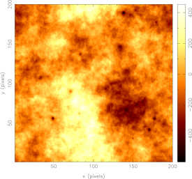
Figure 10: Simulated map of a $5^{\circ}\times 5^{\circ}$ field at 100 GHz. The map consists of the 15 modified King profile SZ clusters shown in Fig. 7 (left panel) and a ‘CMB’ signal with a $C_{\ell}\propto\ell^{-3}$ power spectrum and an rms amplitude of $140$ $\mu$K. The map units are $\mu$K.

Figure 11: Comparison of the true and estimated values of the parameters $X$, $Y$, $A$ and $r_{c}$ for the 12 thermal SZ clusters identified by the McClean algorithm (filled circles). The error bars on the estimated values denote the 68 per cent confidence limits of the corresponding marginalised posterior distribution. The 3 unidentified clusters are represented by the open squares plotted along the bottom of each graph.

We now apply the McClean algorithm to this simulated map, again using 5 Markov chains and taking 500 post burn-in samples from the posterior at each iteration. In this case, the algorithm detects 12 of the 15 objects before terminating. The results are summarised in Fig.11, in which the 12 identified clusters are denoted by the solid circles, and the open squares represent the 3 unidentified clusters. We see that the positions of the identified clusters are once again very accurately constrained. Also, the amplitude $A$ and core radius $r_{c}$ of each identified cluster are recovered to reasonable accuracy, with the scatter about the true values well-described by the derived error-bars. We see that the 3 unidentified clusters are those with the smallest central amplitudes. Moreover, we note that, once again, there are no spurious detections. The burn-in period required for the Markov chains was somewhat shorter for this easier problem, and the entire analysis took around $1$ hour of CPU time on a Pentium III 1 GHz processor.

Let us now compare our results with those obtained by Herranz et al., using their optimal linear pseudofilter and setting a $4\sigma$ detection threshold above the background rms in the filtered domain. Herranz et al. find that the linear filter identifies only 49 per cent of the SZ clusters present, whereas McClean detects 80 per cent; neither method generates spurious detections. To compare the results more closely, we calculate the ‘mean relative error’ in the determination of the cluster amplitudes and core radii. These are defined respectively as

$$\bar{e}_{A}=\frac{1}{N_{\rm d}}\sum_{i=1}^{N_{\rm d}}\frac{|\hat{A}_{i}-A_{i}|}{A_{i}}\quad\mbox{and}\quad\bar{e}_{r_{c}}=\frac{1}{N_{\rm d}}\sum_{i=1}^{N_{\rm d}}\frac{|\hat{r}_{c,i}-r_{c,i}|}{r_{c,i}},$$

where $N_{\rm d}$ is the number of clusters detected. For the linear filter, Herranz et al. found $\bar{e}_{A}=0.104$ and $\bar{e}_{r_{c}}=0.140$, whereas the McClean algorithm gives $\bar{e}_{A}=0.059$ and $\bar{e}_{r_{c}}=0.096$. Thus, we conclude that, on average, McClean determines the amplitude and core radius of the detected clusters with an accuracy almost twice that of the linear filter. Moreover, the Bayesian approach also yields reliable error estimates on the derived parameters.

7.2 The kinetic SZ effect

As stated earlier, the kinetic SZ effect is typically an order of magnitude smaller than the thermal effect. Thus its detection in microwave maps dominated by primordial CMB emission presents an extreme challenge. We note that an optimal linear filtering technique for detecting the kinetic SZ effect embedded in maps of primordial CMB emission has been discussed by Haehnelt & Tegmark (1996).

We shall again consider a simple set of simulated observations, very simliar to those considered in section 7.1.2. Since we are restricting ourselves in this paper to the analysis of simulated observations at a single frequency, we shall consider simulated Planck observations at 217 GHz. At this frequency, the emission due to the thermal SZ effect is zero, and so can be ignored. Moreover, this channel is still in the favourable frequency range where the diffuse Galactic foreground emission is small. Thus, one need only consider the kinetic SZ effect from clusters, embedded in primordial CMB emission (and instrumental noise). We model the kinetic SZ effect using the same 15 cluster profiles as used above for the thermal effect, but now with the central amplitude (in $\mu$K) drawn from the uniform distribution ${\cal U}(-50,50)$. Once again, we assume primordial CMB emission with rms $\sim 100$ $\mu$K. We model the Planck observing beam at 217 GHz by a Gaussian with a FWHM of 5 arcmin, and we assume uncorrelated instrumental pixel noise with rms $20$ $\mu$K.

7.2.1 Evaluation of the posterior distribution for each cluster

Since the kinetic SZ effect is of such small amplitude as compared with the primordial CMB emission, we cannot hope to detect the clusters in the same straightforward way as we did for the thermal effect. Nevertheless, a reasonable strategy does present itself. Since we have already detected and characterised the thermal SZ emission in 7 of the clusters, we can assume the position $(X,Y)$ and core radius $r_{c}$ obtained for each of these clusters and attempt to recover only the amplitude $A$ of the kinetic effect in each cluster individually.

By adopting this strategy, we effectively reduced our problem to determining the 1-dimensional posterior distribution $\Pr(A|\widetilde{D},\hat{X},\hat{Y},\hat{r}_{c})$. In this case there is no need to perform MCMC sampling from the posterior or to locate its global maximum using a simulated annealing approach. Since it is 1-dimensional, one can efficiently evaluate the posterior directly at a regular set of points along the $A$-axis. These posterior distributions can then be used to obtain a ‘best’ estimate $\hat{A}$ of the central kinetic SZ amplitude in each cluster (for example, the peak or the mean of the posterior), and to place confidence limits on our estimate.

Figure 12: Comparison of the true and estimated values of the central kinetic SZ amplitude $A$ for the 7 clusters identifed earlier by their thermal SZ effects, obtained from simulated 217GHz Planck data with a noise rms of 20 $\mu$K (left panel) and 5 $\mu$K (right panel). The solid circles denote the mean of the 1-dimensional posterior distribution for $A$ for each cluster, whereas the error-bars represent the 68 per cent confidence limit in each case.

We perform this procedure for the 7 clusters identified above from their thermal SZ effect. For each cluster, the evaluation of the 1-dimensional posterior for $A$ requires only a few seconds of CPU time. The results are plotted in Fig. 12 (left panel), in which the solid circles represent the mean of the posterior for each cluster and the error-bars represent the 68 per cent confidence limits. The left panel shows the results obtained for a realistic instrumental noise level of 20 $\mu$K per pixel, whereas the right panel corresponds to an artificially low noise level of 5 $\mu$K per pixel. In the former, we see that the recovery central kinetic SZ amplitudes is quite poor. The estimated amplitudes do follow the true amplitudes, but with a large scatter. Indeed, the typical error in the recovered amplitude is $\sim 50$ $\mu$K. In the lower noise case, however, the recovery is better, with a typical error of $\sim 25$ $\mu$K. Even in this extremely optimistic case, however, using the kinetic SZ effect to determine bulk flows in the Universe will be a challenging task for the Planck mission.

7.2.2 Comparison with linear filtering techniques

We may straightforwardly compare our results with those obtained using the linearly-optimal Fourier-filtering technique proposed by Haehnelt & Tegmark (1996) for recovering the kinetic SZ effect in microwave maps dominated by primoridial CMB anisotropies.

For a typical cluster, the central kinetic SZ amplitude is

$$A\approx 30\left(\frac{n_{\rm e}}{3\times 10^{-3}~{}\mbox{cm${}^{-3}$}}\right)\left(\frac{R_{\rm c}}{0.4~{}\mbox{Mpc}}\right)\left(\frac{v_{\rm p}}{500~{}\mbox{km s${}^{-1}$}}\right)~{}\mbox{$\mu$K},$$ (25)

where $n_{\rm e}$ is the electron density in the core, $R_{\rm c}$ is the core radius and $v_{\rm p}$ is the radial peculiar velocity of the cluster. This corresponds to a central optical depth due to electron scattering for the cluster of $\tau\approx 0.005$. Haehnelt & Tegmark show (in their Fig. 3a) that, for an instrumental noise rms of $\sim 6$ $\mu$K per 5 arcmin beam (which is equivalent to 20 $\mu$K per 1.5 arcmin pixel) and projected cluster core radii in the range 1–3 arcmin, the $1\sigma$ error in determining the peculiar velocity of the cluster is

$$\Delta v_{\rm p}\approx 400\left(\frac{\tau}{0.02}\right)^{-1}~{}\mbox{km s${}^{-1}$}.$$

Thus, for a typical cluster with $\tau\approx 0.005$, one obtains $\Delta v_{\rm p}\approx 1600$ km s^-1. From (25), this translates into an uncertainty in the central kinetic SZ amplitude of $\Delta A\approx 100$ $\mu$K. Comparing this value with the typical error $\Delta A\approx 50$ $\mu$K obtained by McClean, we see that the Bayesian approach is again around twice as sensitive as the optimal linear filter.

7.3 Future analysis of real Planck data

So far, we have considered the simple case of detecting circularly-symmetric SZ clusters (with a simple modified King profile) embedded in a background consisting of correlated (CMB) and uncorrelated (instrumental noise) homogeneous Gaussian random fields, observed at a single frequency. Clearly, this is a considerable simplification of the situation one is likely to encounter in the future analysis of real Planck data. Several complications (or generalisations) need to be considered, of which the most important are: (i) the Planck instrument will observe at numerous different frequencies; (ii) at some frequencies there will be significant non-Gaussian, non-stationary emission from Galactic foregrounds; (iii) the instrumental noise will be non-stationary.

Let us first consider point (i). The presence of observations at numerous frequencies brings both advantages and disadvantages to the detection of SZ clusters. Clearly, the well-defined frequency spectrum of the thermal SZ effect allows one to use multifrequency observations to great effect in detecting clusters. Indeed, techniques that make use of multifrequency data in this way have already been proposed for detecting thermal SZ clusters in Planck data (Diego et al. 2001, Herranz et al. 2002b). The extension of the Bayesian approach presented here to multifrequency observations will be presented in a forthcoming paper.

Multifrequency observations do, however, naturally lead to consideration of point (ii) above, namely the presence of foregrounds. The main theoretical difficulty in dealing with foreground emission, such as Galactic synchrotron or dust emission, is that, unlike the CMB, they are most likely to be non-Gaussian and non-stationary. Similarly, any non-stationarity in the instrumental noise field, as mentioned in point (iii) above, will cause corresponding problems.

From section 7.1.1, we see that the Bayesian method assumes knowledge of the functional form of the likelihood function. Moreover, in order to evaluate this function quickly in Fourier space, one assumes that the background (CMB, Galatic components and noise) is stationary, so that its correlation structure can be described entirely in terms of a power spectrum. It must also be noted, however, that the same assumptions are required in the derivation of the optimal linear filters proposed thus far. The assumption of stationary is usually explicit (see e.g. Sanz et al. 2001), but by requiring the variance of the filtered background to be minimised, the notion of Gaussian distributed errors is also implicitly introduced.

For the Bayesian approach, the problem of non-Gaussianity can be addressed directly by simply adopting the appropriate likelihood function (if known). Nevertheless, even for highly non-Gaussian fields such as a dust map, we find (as a result of the central limit theorem) that the probability distribution of its Fourier modes is reasonanly well-described by a Gaussian. We therefore expect the non-Gaussianity of the background will not pose severe problems for either the Bayesian or linear-filter object detection methods. Potentially more serious is the non-stationary of the background. This leads to correlations between Fourier modes, so that the covariance matrix N in (21) is no longer diagonal. Although, in principle, these correlations could be included explicitly (if known), the evaluation of the resulting likelihood function would be computationally more demanding (although not impossible). It has been demonstrated, however, that neglecting inter-mode correlations does not significantly reduce the accuracy of reconstructions in diffuse component separation (see e.g. Stolyarov et al. 2002), and one would expect the same to be true for discrete object detection. In any case, one may easily investigate the effects non-stationarity and non-Gaussianity of the background through simulations. As mentioned above, a detailed account of the issues associated with identifying SZ clusters in multifrequency simulated Planck observations will be presented in a future paper.

8 Conclusions

In this paper, we have presented a Bayesian approach for detecting and characterising the signal from discrete objects embedded in a diffuse background, which is a generic problem in many areas of astrophysics and cosmology. Although our general approach is applicable to datasets of arbitrary dimensionality, we have illustrated our discussion by focussing on the important specific example of detecting discrete objects in a diffuse background in a two-dimensional image.

The traditional approach to this problem has been to apply linear filtering techniques. Typically the filter is optimised for the detection of objects with a given spatial template, although several different filters may be necessary if the objects vary in size and shape. In these approaches, however, the distinction between the filtering and object-detection steps is somewhat arbitrary, and the filtering process itself is only optimal among the rather limited class of linear filters.

The Bayesian approach presented in this paper also assumes a parametrised form for the objects of interest, but the optimal values of these parameters, and their associated errors, are obtained in a single step by evaluation of their full posterior distribution, given the data. If available, one may also place physical priors on the parameters defining an object and on the number of objects present. This technique provides the theoretically-optimal method for parametrised object detection and characterisation. Moreover, owing to its general nature, the method may be applied to a wide range of astronomical datasets.

Within the Bayesian framework, two alternative strategies are investigated: the simultaneous detection of all the discrete objects in the image, and the iterative detection of objects one-by-one. In both cases, the parameter space characterising the object(s) is explored using Markov-Chain Monte-Carlo (MCMC) sampling. The specific implementation of the MCMC technique used is that provided by the Bayesys software. We find that, although the simultaneous detection of all objects present is the theoretically most desirable approach, it requires a complicated MCMC algorithm with the ability to sample from subspaces of different dimensionality. We illustrate the technique by application to a toy problem in which Gaussian-shaped objects are embedded in uncorrelated pixel noise. We find that it performs well, but is also extremely computationally demanding.

In the iterative approach, one attempts to detect and characterise the objects one-by-one. Thus at each iteration, the model for the data contains just a single parametrised object. In this way, the dimensionality of the parameter space is fixed and, generally, small. This allows much more rapid MCMC sampling from the posterior distribution. Indeed, one is interested only in the shape of the posterior distribution around its global maximum, and so fewer samples are required. Once the dominant object has been detected and characterised, it is subtracted from the data and the process is repeated. The iterations are halted when the Bayesian evidence for the ‘detected’ object falls below the evidence for there being no objects left in the image. We call this approach the McClean algorithm. On applying this iterative algorithm to the toy problem, we find that it performs equally well as the simultaneous approach and is computationally much faster.

For the iterative detection of objects, another approach is simply to locate the global maximum of the posterior at each iteration using a simulated annealing simplex technique. We call this algorithm MaxClean. When applied to the toy problem, we find that it yields results very similar to those obtained by McClean, and is computationally faster still. This algorithm also has the advantage of being easily implemented using only standard, readily-available numerical algorithms.

A cosmological illustration of the iterative approach is also presented, in which the thermal and kinetic Sunyaev-Zel’dovich effects from clusters of galaxies are detected in microwave maps dominated by emission from primordial cosmic microwave background anisotropies. We restricted our attention to the analysis of simulated single frequency data from the forthcoming Planck mission. In particular, we found that using only simulated data from the HFI 100 GHz channel, the McClean algorithm is able to detect clusters with central thermal SZ decrements $A\la-250$ $\mu$K and core radii $r_{c}\ga 1$ arcmin.

Once the position and core radius of each cluster has been determined from its thermal SZ signature, we investigate using these values to place constraints on the kinetic SZ in the detected clusters. Using simulated Planck observations at 217 GHz, where the thermal effect is negligible, and assuming realistic instrumental noise with an rms $\sim 20$ $\mu$K per pixel, we found that the amplitude of the kinetic effect can only be determined to an accuracy of $\sim 50$ $\mu$K. Assuming a very optimistic noise rms of $\sim 5$ $\mu$K, this error can only be reduced to $\sim 25$ $\mu$K.

In general, it is unnecessary to restrict our attention to the analysis of a single astronomical image, such as a map at a particular observing frequency. In many cases, several different images may be available, each of which contain information regarding the discrete object of interest. For example, forthcoming CMB satellite missions, such as the Planck experiment, should provide high-sensitivity, high-resolution observations of the whole sky at a number of different observing frequencies. Owing to the distinctive frequency dependence of the thermal SZ effect, it is better to use the maps at all the observed frequencies simultaneously when attempting to detect and characterise thermal SZ clusters hidden in the emission from other astrophysical components. The application of our Bayesian approach to more realistic multi-frequency simulated Planck observations will be presented in a forthcoming paper.

Finally, as mentioned in section 6.1.1, the iterative approach to object detection, exemplified by the McClean and MaxClean algorithms, is a compromise between using the fully Bayesian approach, in which the objects are identified simultaneously, and the desire to obtain results in a reasonable amount of CPU time. As we have shown, this simple iterative approach may be successfully applied to problems in which the objects of interest are well-localised and the data are such that the determination of the characteristics of one object does not significantly affect the derived properties of any other. In an astronomical context, this is clearly the case for well-separated SZ clusters observed by experiments for which the beam is narrow and has negligible side-lobes, such as the Planck mission. Since the iterative approach does, however, represent only a convenient approximation to the fully Bayesian simultaneous detection of objects, there will inevitably be (common) situations for which it will perform less well.

A simple astronomical example of such a case is provided by interferometric observations, for which the synthesised beam often has non-negligible sidelobes of large spatial extent. Using the SZ effect as an example, in this case the observed flux of a given cluster would contain contributions from other clusters lying in the side-lobes of the synthesised beam. This would lead to the basic iterative algorithm either over- or underestimating the flux of the cluster, depending on the positions and amplitudes of the other clusters with respect to the sidelobe structure. Nevertheless, a simple modification of the basic iterative algorithm easily addresses this difficulty. Once a set of objects have been identified and characterised by the McClean (or MaxClean) algorithm, one can refine the estimates of the parameters of the objects as follows. For each object in turn, one re-runs the MCMC (or global maximisation) algorithm to explore the parameter space $\{X_{k},Y_{k},A_{k},R_{k}\}$, but this time including the other (fixed) derived objects in the model of the data. This allows the defining parameters of the $k$th object to be refined in the presence of the other detected objects $(k^{\prime}\neq k)$. By repeating this procedure until convergence is obtained, one thus obtains a joint optimal set of defining parameters for the objects, thereby circumventing the problem identified above. The application of this extended iterative procedure to simulated interferometer observations of the SZ effect in clusters will be presented in a forthcoming paper.

ACKNOWLEDGMENTS

We thank John Skilling for providing the Bayesys software and Steve Gull for helpful advice regarding its use. The authors also acknowledge NESTA for their financial support of this work.

References

- [] Bertin E., Arnouts S., 1996, A&AS, 117, 393
- [] Chiang L.-Y., Jorgensen H.E., Naselsky I.P., Naselsky P.D., Novikov I.D., Christensen P.R., 2002, MNRAS, submitted (astro-ph/0202399)
- [] Christensen N., Meyer R., Knox L., Luey B., 2001, Class. Quant. Grav., 18, 2677
- [] Cowles M.K., Carlin B.P., 1994, Technical Report 94-008, Division of Biostatistics, School of Public Heath, University of Minnesota
- [] Diego J.M., Vielva P., Martínez-González E., Silk J., Sanz J.L., 2001, MNRAS, submitted (astro-ph/0110587)
- [] Eaton M.L., 1983, Multivariate Statistics. Wiley, New York
- [] Gilks W.R., Richardson S., Spiegelhalter D.J., 1995, in eds Gilks W.R., Richardson S., Spiegelhalter D.J., Markov Chain Monte Carlo in Practice. Chapman & Hall, London.
- [] Green P.J., 1994, J. R. Statist. Soc., 56, 589
- [] Haehnelt M.G., Tegmark M., 1996, MNRAS, 279, 545
- [] Hobson M.P., Lahav O., Bridle S.L., 2002, MNRAS, in press (astro-ph/0203259)
- [1] Herranz D, Sanz J.L., Barreiro R.B., Martínez-González E., 2002a, ApJ, submitted (astro-ph/0204149)
- [2] Herranz D, Sanz J.L., Hobson M.P., Barreiro R.B., Diego J.M., Martínez-González E., Lasenby A.N., 2002b, MNRAS, submitted (astro-ph/0203486)
- [] Kalos M., Whitlock P., 1986, Monte Carlo Methods. Wiley, New York
- [] Knox L., Christensen N., Skordis C., 2001, ApJ, 563, L95
- [] Ó’Ruanaidh J.J.K., Fitzgerald W.J., 1996, Numerical Bayesian Methods Applied to Signal Processing. Springer-Verlag, New-York
- [] Philips D.B., Smith A.F.M., 1995, in eds Gilks W.R., Richardson S., Spiegelhalter D.J., Markov Chain Monte Carlo in Practice. Chapman & Hall, London.
- [] Press W.H., Teukolsky S.A., Vetterling W.T., Flannery B.P., 1994, Numerical Recipies in Fortran 77. Cambridge University Press
- [] Sanz J.L., Herranz D., Martínez-González E., 2001, ApJ, 552, 484
- [] Seljak U., Zaldarriaga M., 1996, ApJ, 469, 437
- [] Sivia D.S., 1996, Data Analysis: A Bayesian Tutorial. Oxford University Press
- [] Skilling J., 2002, in preparation
- [] Stetson P.B., 1992, User’s Manual for Daophot II, available at http://www.ast.cam.ac.uk/m̃bt/daophot
- [] Stolyarov V., Hobson M.P., Ashdown M.A.J., Lasenby A.N., 2002, MNRAS, in press (astro-ph/0105432)
- [] Zhang P., Pen U.L., Wang B., 2002, ApJ, submitted (astro-ph/0201375)