Using peak distribution of the cosmic microwave background for WMAP and Planck data analysis: formalism and simulations

We implement and further refine the recently proposed method (Kashlinsky, Hernández-Monteagudo & Atrio-Barandela, 2001 - KHA) for a time efficient extraction of the power spectrum from future cosmic microwave background (CMB) maps. The method is based on the clustering properties of peaks and troughs of the Gaussian CMB sky. The procedure takes only $\frac{1}{2}[f(\nu)]^{2}N^{2}$ steps where $f(\nu)$ is the fraction of pixels with $|\delta T|\geq\nu$ standard deviations in the map of $N$ pixels. We use the new statistic introduced in KHA, $\xi_{\nu}$, which characterizes spatial clustering of the CMB sky peaks of progressively increasing thresholds. The tiny fraction of the remaining pixels (peaks and troughs) contains the required information on the CMB power spectrum of the entire map. The threshold $\nu$ is the only parameter that determines the accuracy of the final spectrum. We performed detailed numerical simulations for parameters of the two-year WMAP and Planck CMB sky data including cosmological signal, inhomogeneous noise and foreground residuals. In all cases we find that the method can recover the power spectrum out to the Nyquist scale of the experiment channel. We discuss how the error bars scale with $\nu$ allowing to decide between accuracy and speed. The method can determine with significant accuracy the CMB power spectrum from the upcoming CMB maps in only $\sim(10^{-5}-10^{-3})\times N^{2}$ operations.

1 Introduction.

The sub-degree structure of the CMB probes linear scales that were inside the horizon at the last scattering epoch. The CMB fluctuations on these scales carry a signature of causal processes during the last scattering and thereby provide a very important constraint on the physics of the early Universe and the models for structure formation. The most popular of these models is the cold dark matter (CDM) set of models based on the inflationary paradigm for the evolution of the early Universe. The models are very appealing, not only because of their relative simplicity, but also because they provide a clear-cut set of predictions that can be verified by observations. One (and perhaps the most critical) of these predictions is the sub-degree structure of the CMB anisotropies. In the framework of CDM models with adiabatic density fluctuations the structure of the CMB power spectrum reflects the linear physics of sound waves and initial density perturbations. While on scales outside the horizon at de-coupling the CMB field preserves the initial power spectrum, on sub-degree scales the interaction between the photon fluid and matter leads to a series of acoustic peaks. The relative height, width and spacing of these peaks depend on a final set of the cosmological parameters ($\Omega_{\rm total},\Omega_{\Lambda},\Omega_{\rm b},h$) and also serve to validate the cosmological CDM paradigm (see Hu & Dodelson 2002 for a recent review). It is then important to measure the sub-degree structure of the CMB with high accuracy.

After its first year of operation, the WMAP experiment has measured the Cosmic Microwave Background (hereafter CMB) at five different frequencies with the maximal angular resolution of $\sim 0.21\degr$ and sensitivity close to $175\leavevmode\nobreak\ {\rm\mu K}$ per 7’ pixel, (Bennet et al. 2003a). With these sensitivity and angular resolution levels, the cosmological parameters as $\Omega_{0}$, $\Omega_{\Lambda}$, $\Omega_{\rm baryon}$, $H_{0}$, $n$, $\tau_{\rm reio}$ were determined with high accuracy (Spergel et al 2003). These measurements should be further improved with the planned ESA’s mission Planck, where maps will contain up to $10^{7}$ pixels and extend to higher angular resolution. Angular resolution and noise are both important for determining the cosmological parameters from the CMB.

A major challenge to understanding current and future CMB measurements is to find an efficient algorithm that can reduce these enormous datasets: $N\!\simeq\!10^{5}$ pixels in balloon experiments, $\simeq\!3\times 10^{6}$ for WMAP, to $\simeq\!5\!\times\!10^{7}$ for the Planck HFI data. (For comparison the COBE DMR data analysis was based on only 4,144 pixels). Traditional methods require inverting the covariance matrix and need $\sim\!N^{3}$ operations making them unfeasible for the current generation of computers. Thus alternatives have been developed for estimating the CMB multipoles from Gaussian sky maps: Tegmark (1997) proposed a least variance method that yields $C_{l}$’s directly from the temperature map in O($N^{2}$) operations, while Oh, Spergel & Hinshaw (1999, hereafter OSH) perform an iterative maximization of the likelihood of the temperature map, also in O($N^{2}$) operations. The first year WMAP results were analyzed with the OSH method (Hinshaw et al 2003). Bond, Jaffe & Knox (2000) and Wandelt, Hivon & Górski (2001) concentrate on the statistics of $C_{l}$’s, once the temperature map has been Fourier transformed. Hivon, et al. (2002) studied the likelihood of the power spectrum as obtained by direct Fast Fourier Transform of the available portion of the sky. Though it requires $O(N^{3/2}\ln N)$ operations, the accuracy of their results depends on the fraction and geometry of the sky covered. A different approach consists in computing the correlation function directly from the data in $O(N^{2})$ operations. Smoot et al. (1992) used this type of analysis for the first year release of the COBE data. More recently, Szapudi et al. (2001), Szapudi, Prunet & Colombi (2001) have developed it for mega-pixel CMB data sets. The last contribution in this field comes from Penn (2003), who applies existing (Padmanabhan, Seljak & Penn 2002) iterative algorithms on CMB data analysis, and manages to estimate to power spectra in ${\cal O}$(N log N) operations.

A different method to compute the CMB power spectrum in a fast and accurate manner was proposed by us (Kashlinsky, Hernández-Monteagudo & Atrio-Barandela, 2001, hereafter KHA). The method exploits Gaussian properties of the CMB and noise fields and uses high peaks (and troughs) of the CMB field whose abundance is much smaller than the total number of pixels, $N$, and whose correlation properties are strongly amplified in a way that depends on the underlying power spectrum. This simultaneously achieves two important goals: reducing the number of computational steps for analysis and the good accuracy of the measured parameters. KHA have shown that the tiny fraction of the remaining pixels (peaks and troughs) contains the required information on the CMB power spectrum in the small scales. The peaks also trace, by default, the pixels with high signal-to-noise ratio and keep most of the information about the power spectrum of the signal. Although this method may not provide as accurate results as other more time consumings methods, it provides a new, non-standard and independent tool to unveil the sub-degree structure of the CMB.

In this paper we present detailed numerical simulations with the application of the KHA method to WMAP and Planck datasets in the presence of realistic components, such as inhomogeneous noise and non-Gaussian features expected from the Galactic foreground residuals. We show that with this method we can determine the CMB power spectrum outside the beam ($l\!\simeq\!640$ for WMAP and higher for Planck) in only $<\!10^{-3}N^{2}$ operations. We show that for the projected two-year WMAP noise levels our error bars at each $l$ are, on average, comparable to OSH, but have larger correlations which may be a small price to pay for the significantly shorter computational time. For both WMAP and Planck parameters the KHA method is also faster than the direct computation of the CMB power spectrum in $O(N^{3/2}\log N)\sim N^{1.61}$ steps.

The structure of this paper is as follows: In Sect. 2 we briefly review the KHA formalism and in Sect. 3 we discuss its numerical implementation. Sect. 4 deals with application of the method to both idealized and realistic WMAP data. We show there that the method is immune to noise inhomogeneities and non-Gaussian features of Galactic foregrounds. Sect. 5 follows with results for application of the KHA method to Planck and in Sect. 6 we present our main conclusions.

2 Mathematical formalism: an overview

For completeness we give a brief overview of the KHA method; more details are in KHA.

The CMB sky is expected to be highly Gaussian (Komatsu et al 2003) and this property, Eq. (1) below, is also widely used in standard maximum likelihood methods. For a Gaussian ensemble of $N$ data points (e.g. pixels) describing the CMB data $\delta\equiv T-\langle T\rangle$ one will find a fraction $f(\nu)=$erfc($\nu/\sqrt{2})$ with $|\delta|\geq\nu\sigma$, where $\sigma^{2}=\langle\delta^{2}\rangle$ is the variance of the field and erfc is the complementary error function. The fraction of peaks, $f(\nu)$, is a rapidly decreasing function for $\nu{{}_{>}\atop{}^{\sim}}1$ and is e.g. $f(\nu)=(4.5,1,0.1)\times 10^{-2}$ for $\nu=(2,2.5,3)$ respectively. The joint probability density of finding two pixels within $d\delta_{1,2}$ of $\delta_{1,2}$ and separated by the angular distance $\theta$ is given by the bivariate Gaussian:

$$p(\delta_{1},\delta_{2})=\frac{1}{2\pi\sqrt{||\mbox{\boldmath$C$}||}}\exp(-\frac{1}{2}\mbox{\boldmath$\delta$}\cdot\mbox{\boldmath$C$}^{-1}\cdot\mbox{\boldmath$\delta$})$$ (1)

where $C$ is the covariance matrix of the temperature field. We model the temperature correlation function (or matrix, if defined on a set of pixels) as

$$C(\theta_{ij})=C^{\rm CMB}(\theta_{ij})+\langle{\cal N}_{i}{\cal N}_{j}\rangle$$ (2)

where $C^{\rm CMB}(\theta_{ij})$ and $\langle{\cal N}_{i}{\cal N}_{j}\rangle$ are the CMB and the noise correlation matrices, respectively. We further define the total variance of the map as $C_{0}\equiv C^{\rm CMB}(0)+\langle{\cal N}^{2}\rangle$. The case of inhomogeneous noise, i.e., noise whose variance varies across the sky, will be discussed in Sect. 4.2. Note that the power spectrum of the map is nothing but the Legendre transform of $C(\theta)$, (see Eq. (5) below).

The distribution of peaks of a Gaussian field is strongly clustered (Rice 1954, Kaiser 1984, Jensen & Szalay 1986, Bardeen et al. 1986, Kashlinsky 1987). Their angular clustering can be characterized by the 2-point correlation function, $\xi$, describing the excess probability of finding two events at the given separation. The correlation function of such regions is:

$$\xi_{\nu}(\theta)=\frac{2\int_{\nu\sigma}^{\infty}\int_{\nu\sigma}^{\infty}[p(\delta_{1},\delta_{2})+p(-\delta_{1},\delta_{2})]d\delta_{1}d\delta_{2}}{[2\int_{\nu\sigma}^{\infty}p(\delta)d\delta]^{2}}-1=A_{\nu}(\frac{C}{C_{0}})$$ (3)

where $A_{\nu}$ is evaluated in detail in KHA to be:

$$A_{\nu}(x)=\frac{1}{H^{2}_{-1}(\frac{\nu}{\sqrt{2}})}\sum_{k=1}^{\infty}\frac{x^{2k}}{2^{2k}(2k)!}H_{2k-1}^{2}(\frac{\nu}{\sqrt{2}})$$ (4)

Here $H_{n}(x)=(-)^{n}\exp(x^{2})d^{n}/dx^{n}\exp(-x^{2})$ is the Hermite polynomial; $H_{-1}(x)\equiv\frac{\sqrt{\pi}}{2}\exp(x^{2})$erfc($x)$.

At each angular scale the value of $\xi_{\nu}$ for every $\nu$ is determined uniquely by $C$ at the same angular scale. In the limit of the entire map ($\nu$=0) our statistic is $\xi_{\nu}$=0 and our method becomes meaningless; the new statistic has meaning only for sufficiently high $\nu$. One should distinguish between the 2-point correlation function, $\xi$, we directly determine from the maps, and the commonly used statistics in CMB studies, the temperature correlation function, $C$.

KHA thus suggested the following procedure to determine the power spectrum of CMB in only $\simeq\!f^{2}(\nu)N^{2}\!\ll\!N^{2}$ operations:

1. Determine the variance of the CMB temperature, $C_{0}$, from the data in $N$ operations;

2. Choose sufficiently high value of $\nu$ when $f(\nu)$ is small but at the same time enough pixels are left in the map for robust measurement of $\xi_{\nu}(\theta)$;

3. Determine $\xi_{\nu}(\theta)$ in $[f(\nu)]^{2}N^{2}$ operations.

4. Finally, solve the equation $A_{\nu}(C/C_{0})\!=\!\xi_{\nu}(\theta)$ to obtain $C^{\rm CMB}(\theta)$ and from it $C_{l}$. This last step assumes that the experimental noise correlation function $\langle{\cal N}_{i}{\cal N}_{j}\rangle$ has been properly determined, at least in the set of pixels selected in the analysis, so that it can be subtracted from the total correlation function $C(\theta_{ij})$.

Formally speaking this procedure would require $\frac{1}{2}[f(\nu)]^{2}N^{2}$ operations because of the symmetry in counting pairs. For simplicity we will be referring to this as O$(f^{2}N^{2})$ method implying a gain factor of $[f(\nu)]^{2}$ compared to other O$(N^{2})$ methods.

3 Numerical implementation

3.1 Modeling the CMB sky

Maps of the CMB sky were generated using the hierarchical equal area isolatitude pixelization of the celestial sphere implemented in HEALPix. Pixels have equal area and are arranged in “constant latitude rings”. Maps can be constructed with varying resolution, the number of pixels given by $N=12\times N_{\rm side}^{2}$, being $N_{\rm side}$ the number of times in which each side of a pixel will be divided in two, starting from a given initial configuration. For a value of $N_{\rm side}$ of 512, one generates a map of 3,145,728 pixels of size of seven arcminutes. In the case of PLANCK, we used $N_{\rm side}=1024$ or 12,582,912 pixels of 3.5 arcminutes size. The CMB spectrum was obtained using the CMBFAST code (Seljak & Zaldarriaga, 1996).

For WMAP and PLANCK, we performed two types of simulations including: (1) cosmological signal plus white noise, and (2) cosmological signal, foregrounds and inhomogeneous white noise. We chose three different thresholds: $\nu=2.0,2.27,2.525$ for WMAP and $\nu=2.55,2.78,3.0$ for Planck. At each threshold, the pixels selected are (on average) $f(\nu)N$ and their number doubles with decreasing threshold. The thresholds for WMAP and Planck were chosen such that they select the same number of pixels in both experiments. In this way, we can analyze the effect of pixel number on the accuracy of the method, i.e., we can estimate how the multipole error bars scale with threshold.

From the peak spatial distribution, $\xi_{\nu}(\theta)$ was computed on a grid of 31,415 equally spaced bins. The power spectrum is computed using a Gauss-Legendre integration:

$$C_{l}=2\pi\int_{0}^{\pi}d\theta\sin\theta C(\theta)P_{l}(\cos\theta).$$ (5)

Accurate integration requires the evaluation of $C(\theta)$ at the roots of the Legendre polynomial out to a maximum order $l_{\rm max}$ (Press et al 1992) and this property was used by Szapudi et al (2001), Szapudi, Prunet, & Colombi (2001) and KHA. The value of $l_{\rm max}=800$ was chosen as a compromise between the beam scale and the pixel angular scale, in order to prevent the first root of the Legendre polynomial from being within the pixel size where there is no information on $\xi_{\nu}(\theta)$. Prior to inverting Eq. (3) $\xi_{\nu}(\theta)$ was smoothed using a Gaussian of width 4’ centered on the roots of the Legendre polynomials. We verified that other average schemes lead to essentially identical results.

Fig. (1a) shows $\xi_{\nu=2}(\theta)$ for a SCDM model, with $\Omega_{\rm total}=1$, $\Omega_{\Lambda}=0$, $\Omega_{\rm b}=0.04$, $H_{0}=55\;{\rm km\;s^{-1}\;Mpc}$ and scalar perturbation spectral index $n_{S}=1$. The solid line corresponds to the theoretical prediction and the dashed line is a smooth average obtained from the data. The agreement is very good out to $\theta\sim 10{{}^{\circ}}$, allowing an accurate reconstruction of the power spectrum in the range of interest: $l{{}_{>}\atop{}^{\sim}}30$.

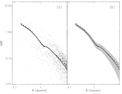
Figure 1: (a) $\xi_{\nu=2}$ for the SCDM model with a Harrison-Zel’dovich power spectrum, obtained from a single realization of WMAP 94GHz channel. Solid line: theoretical estimate (Eq. [3]). Dots: raw data of $\xi_{\nu=2}$ evaluated at 31,415 angular bins distributed uniformly from $\theta=0{{}^{\circ}}$ to $180{{}^{\circ}}$. Dashed line: result of filtering the raw data with a Gaussian of $4^{\prime}$ width at the roots of the Legendre polynomial of order $800$. (b) The shaded area represents the $1\sigma$ optimal variance error bar (eq [6]) for the 94 GHz WMAP channel. Dashed and solid lines have the same meaning as in (a).

3.2 Accuracy of $\xi$ and correlations

There are numerous ways to estimate $\xi_{\nu}(\theta)$ from the data, each way coming with its own uncertainty and systematics. Ideally, the uncertainty in $\xi_{\nu}(\theta)$ should reach $1/\sqrt{N_{\rm pairs}}$ but in practice systematic and other effects become dominant (Peebles 1980). Because the KHA method involves a complex and non-linear algorithm for inverting $C_{l}$’s from $\xi_{\nu}(\theta)$, the accuracy of the resultant CMB power spectrum may depend sensitively on the details, uncertainties and correlations of a particular estimator of $\xi_{\nu}$.

The ultimate accuracy with which the CMB power spectrum can be determined at each $l$ is given by the so called optimal variance containing both the cosmic variance and the instrument noise (Knox 1995):

$$\sigma_{\rm OV}(l)=\sqrt{\frac{2}{(2l+1)f_{\rm sky}}}[C_{l}+\frac{4\pi\langle{\cal N}^{2}\rangle B_{l}^{-2}}{N}].$$ (6)

In this equation, $N$ is the number of pixels, $f_{\rm sky}$ is the fraction of the sky covered by the experiment and $B_{l}$ is the window function due to the finite beam resolution. This uncertainty also limits the accuracy with which one can determine the correlation functions $C$ and $\xi$. The latter are given by:

$$\sigma^{2}_{C(\theta)}=\sum_{l}|\frac{\partial C(\theta)}{\partial C_{l}}|^{2}\sigma^{2}_{\rm OV}(l),\quad\sigma^{2}_{\xi_{\nu}(\theta)}=|\frac{\partial\xi_{\nu}(\theta)}{\partial C(\theta)}|^{2}\sigma^{2}_{C(\theta)}.$$ (7)

The shaded region in Fig. (1) shows an example of the optimal variance uncertainty in $\xi_{\nu=2}(\theta)$. (Note that it is a function of $\nu$).

In KHA, we evaluated $\xi_{\nu}$ as the ratio of number of peak pairs at a given angular scale with respect to a poissonian catalog:

$$\hat{\xi_{\nu}}(\theta)=DD/RR-1.$$ (8)

At each angular separation, $DD$ is the number of pairs of peaks and $RR$ the number of pairs of $f(\nu)N$ points randomly located on the sphere Landy & Szalay (1993) argue that this estimator is neither optimal nor unbiased. They proposed a more accurate estimator defined by:

$$\tilde{\xi_{\nu}}(\theta)=(DD+RR-2DR)/RR,$$ (9)

with $DR$ is the number of pairs given a cross-correlation between the $f(\nu)N$ peaks of the CMB map and the same number of points Poisson distributed on the sky. We performed simulations for WMAP as described in Sect. 4 and computed $\xi_{\nu}$ using both estimators. We found that, for the range of interest ($\theta<10{{}^{\circ}}$), both estimators show scatter equally close to Eq. (7). Hence, in what follows we shall use Eq. (8) to be consistent with KHA.

In Fig. (1b) we plot the 1-$\sigma$ errors in $\xi_{\nu=2}$ for the 94 GHz WMAP channel given by the noise and cosmic variances. The smooth average obtained from the data (dashed line) is in good agreement with theoretical value. Therefore, we will expect that the radiation power spectrum obtained from $\xi_{\nu=2}$ as described below will be very close to that of the input model.

The sampling variance associated with the low number of pairs - compared with methods based on the correlation function - is much smaller that the cosmic variance on $\xi_{\nu}$. Fig. (2) shows $\sqrt{N_{\rm pairs}}\sigma_{\xi,{\rm OV}}$ which is the ratio of the optimal variance uncertainty on $\xi$ to the statistical uncertainty, $1/\sqrt{N_{\rm pairs}}$. The lines correspond to various $\nu$=1.5 (dashes), 2 (dots) and 3 (solid line). The ratio was computed for WMAP number of pixels. The plot shows that for any mega-pixel CMB map the method can determine the new statistic, $\xi_{\nu}$, out to the angles of interest optimally even for threshold as low as $\nu=1.5$. This is the reason why our results are not sensitive to the particular estimator used in calculating $\xi_{\nu}$.

Figure 2: The ratio of the optimal variance uncertainty on $\xi_{\nu}$ to the statistical uncertainty, $1/\sqrt{N_{\rm pairs}}$ plotted vs the separation angle for the resolution of the WMAP 94GHz channel. The solid line corresponds to $\nu=3$, dotted to $\nu=2$ and dashes to $\nu=1.5$.

At $\theta{{}_{>}\atop{}^{\sim}}10{{}^{\circ}}-20{{}^{\circ}}$ the value of $\xi_{\nu}(\theta)$ is small and its value becomes dominated by shot noise. Hence, we restrict the analysis to $\theta<10{{}^{\circ}}-20{{}^{\circ}}$ by introducing a taper function that cuts out the contribution of the correlation function for $\theta{{}_{>}\atop{}^{\sim}}10{{}^{\circ}}$. As a result (a) we will not recover very accurately multipoles below $l\simeq 30$ and (b) tapering will introduce additional correlations among the different $C_{l}$’s. The first limitation is irrelevant, since one can always degrade the map to smaller resolution and apply standard techniques to recover the power spectrum at $l\leq 20-40$. The second limitation is common to all methods that compute the power spectrum by means of the correlation function or in the presence of Galactic (and other) cut. The intrinsic multipoles need to be de-convolved from the tapering function, i.e., if $C^{\rm intrinsic}_{l}$ are the multipoles of the sky radiation power spectrum, and $C_{l}$ are obtained using Eq. (5), then

$$C_{l}=\sum_{l^{\prime}}C^{\rm intrinsic}_{l^{\prime}}{\cal F}_{l-l^{\prime}}$$ (10)

where ${\cal F}_{l}$ is the Legendre transform of the tapering function $F$.

Fig. (3) shows the Legendre transform of the tapering function as function of $\Delta l\equiv l-l^{\prime}$ for Gaussian and top-hat tapering. The advantage of Gaussian tapering is quite obvious as it leads to significantly less prominent side-lobes. Hence, we adopted it in our computations. As the figure shows, it would lead to FWHM correlation width of only $\Delta l\sim$ (a few) for tapering angles ${{}_{<}\atop{}^{\sim}}10{{}^{\circ}}$. Correlations on the $C_{l}$’s would be dominated by tapering and correlated errors on $\xi_{\nu}$.

Figure 3: Legendre transform of the tapering function (Eq. 10) plotted vs $\Delta l=l-l^{\prime}$. Left panel corresponds to Gaussian tapering, $F(\theta)\propto\exp(-\theta^{2}/\theta_{t}^{2})$ and the right panel to the top hat tapering, $F(\theta)=1$ for $\theta\leq\theta_{t}$ and zero otherwise. Dashed, dotted and solid lines correspond to $\theta_{t}=18{{}^{\circ}},12{{}^{\circ}},8{{}^{\circ}}$ respectively.

4 Application to WMAP

WMAP is observing at 5 frequency bands: 23, 33, 41, 61, and 94 GHz, (Jarosik et al. 2003, Bennett et al. 2003a). The beam response at each band are given by a gain pattern, G, which is asymmetric and non-gaussian. From the solid angle beam, one can always define a FWHM, which, for increasing frequency channels, are equal to 0.82, 0.62, 0.49, 0.33 & 0.21 degrees, (Page et al. 2003). The sky maps based on the full two-years of data are expected to have an $rms$ noise of $\simeq$35 $\mu$K per $0.3{{}^{\circ}}\!\times\!0.3{{}^{\circ}}$ pixel. By design, the noise will be essentially uncorrelated from pixel to pixel and it is expected to be highly Gaussian (Hinshaw 2000, Hinshaw et al. 2003). Due to the sky scanning strategy, the noise is reasonably uniform across the sky, except at the small regions near the ecliptic poles and at ecliptic latitude $\sim 45{{}^{\circ}}$ where the sensitivity will be somewhat higher. The WMAP radiometers produce raw temperature measurements that are the differences between two points on the sky separated $\sim 140{{}^{\circ}}$ . Since a given pixel $i$ is observed with up to  1000 different pixels $j$, the covariance between any given pair of pixels $(i,j)$ is much less than 1% of the variance of pixel $i$. The noise covariance in the final sky maps will, by design, be very nearly diagonal.

4.1 Homogeneous noise results

First, we performed a set of 500 simulations for $\nu=(2,2.27,2.525)$ including only cosmological signal and white noise. For each simulation, we computed the correlation function and the power spectrum. Fig. (4) summarizes the results for the threshold $\nu=2$. In panel (a) the dotted line shows the power spectrum recovered from a single simulation, whereas the solid line gives the input power spectrum. Tapering angle was $\theta_{t}=12{{}^{\circ}}$. In (b), we show the average results for 500 realizations: the solid and dashed lines represent the input model and the average power spectrum of the 500 simulations, respectively. The shaded area shows the 1-$\sigma$ error bar region for each $C_{l}$ and the dashed lines show the optimal variance. Our method traces the acoustic peaks up to the beam scale, $l_{\rm beam}\sim 640$. Its accuracy is roughly similar to the optimal variance $\sigma_{\rm OV}$ for $l\leq 300$. The spectrum of Fig. (4a) has been obtained in $10^{-3}N^{2}$ operations, using a taper window of $12{{}^{\circ}}$ FWHM. The accuracy can be improved by lowering the threshold $\nu$ and hence increasing the computational time.

To see the effect of tapering, in Fig. (4c) we plot the power spectra obtained for two different tapering angles for the same simulation as in Fig. (4a). The solid line corresponds to $\theta_{t}=8{{}^{\circ}}$ while the dashed line to $\theta_{t}=18{{}^{\circ}}$. Increasing the tapering angle leads to larger oscillations, but also decreases the correlations between different $l$. In Fig. (4d) we plot the band power average of the previous spectra: diamonds correspond to the tapering angle of $8{{}^{\circ}}$ and triangles to $18{{}^{\circ}}$. The solid line is the input model and the dashed lines correspond to the optimal variance error bars as in (b). As expected, both results are almost identical since all the information at high $l$’s is contained at angular scales smaller than $1{{}^{\circ}}$.

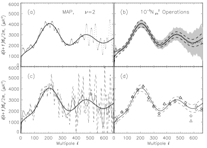
Figure 4: Radiation power spectrum for $\nu=2$ and different taper angles. In all panels the solid line shows the input power spectrum. (a) Dotted line: power spectrum obtained from a single simulation with $\theta_{t}=12^{0}$. (b) Dotted line: power spectrum obtained from averaging 500 simulations, shaded area: 1$\sigma$ error region obtained from the same simulations. The dashed lines limit the 1$\sigma$ optimal variance error bars (Eq. (6)). (c) The same as in (a) but for $\theta_{t}=8^{0}$ (solid line) and $\theta_{t}=18^{0}$ dashed line. (d) solid and dashed lines as in (b); the symbols displayed the band averaged power spectra with bandwidth $\Delta l=40$ of the spectra plotted in (c): diamonds correspond to $\theta_{t}=8^{0}$ and triangles to $\theta_{t}=18^{0}$.

The correlation matrix, ${\cal C}_{l,l^{\prime}}$, among different multipoles is given by:

$${\cal C}_{l,l^{\prime}}=\frac{\langle\delta C_{l}\delta C_{l^{\prime}}\rangle}{\sqrt{\langle\delta C_{l}^{2}\rangle\langle\delta C_{l^{\prime}}^{2}\rangle}},$$ (11)

with $\delta C_{l}=C_{l}-\langle C_{l}\rangle$. The correlation coefficient matrix has been computed after using a Gaussian taper function $F(\theta)=\exp-(\theta/\theta_{t})^{2}$. It is highly diagonal with FWHM width $\Delta l\sim 10$ for $\theta_{t}=8{{}^{\circ}}$, independently of the value of the multipole $l$. At $\Delta l\sim 20$ the correlation drops to the level of $\sim 5\%$, independently of $\nu$. Outside the central diagonal strip the residual correlations are due to shot noise from the finite number of simulations. For consistency, we repeated the analysis with only 125 simulations. The width of the diagonal remained the same, but the off-diagonal terms grew by a factor of two, consistent with Poisson statistics.

For larger/smaller tapering angles, the correlation scale $\Delta l$ will be smaller/larger but, as demonstrated in Fig. (4d), it will not change our estimate of the power spectrum. We also checked that our results did not change if we use the correlation function from the coarser (and computationally tractable) map from $\theta=10{{}^{\circ}}$ out to $180{{}^{\circ}}$ instead of tapering. The correlation on the final $C_{l}$’s are dominated by the correlated errors in $\xi_{\nu}$ at small angles.

In Fig. (5) we compare the accuracy of our method for WMAP and $\nu=2$ with that of OSH. We compute the ratio of the uncertainties in the multipoles recovered by both methods. Our method gives a comparable precision to that of OSH but requires much fewer operations. On the other hand, it gives fewer independent data points. In direct methods, such as OSH, the necessary Galactic cut leads to $C_{l}$’s that are correlated on scales of $\Delta l\simeq 2-3$, while our method gives a correlation length of about $\Delta l\sim 10$.

Figure 5: Comparison of the error bars of OSH and KHA methods for a CMB map as seen by the 94 GHz channel of WMAP. We plot the ratio $(\sigma_{C_{l}})_{\rm KHA}/(\sigma_{C_{l}})_{\rm OSH}$. The uncertainties $\sigma_{C_{l}}$’s were computed for raw multipole estimates $C_{l}$, without averaging.

In Fig. (6) we show the variation of the error bar with bandwidth for the multipole at $l=200$. Solid, dashed and dotted lines correspond to $\nu=2.5,2.27$ and $2$, respectively. Due to the presence of this correlation among the multipole estimates, this $\sigma_{C_{l}}\sim(\Delta l)^{-1/2}$ behavior is obtained for $\Delta l{{}_{>}\atop{}^{\sim}}10$, the correlation scale introduced by our method.

Figure 6: Scaling of band power error bar $\sigma_{C_{l}}$ with bandwidth $\Delta l$. Solid, dashed and dotted lines correspond to $\nu=2.5,2.27$ and $2$, respectively.

In Fig. (7) we show $\sigma_{C_{l}}$ at $l=200,300,400,500$ for the three thresholds. Smaller error bars correspond to smaller thresholds, i.e., to larger number of peaks. A power-law fit using all multipoles gives a power law behavior of the form $\sigma_{C_{l}}\propto N_{\rm peaks}^{\beta}$, with $\beta=-0.405\pm 0.016$. These relations can be used to estimate the amplitude of the error bar attached to each multipole for a wide range of values of $\nu$ and $\Delta l$. In particular, it can be used to find what values of $\nu$ and $\Delta l$ are necessary to achieve a given degree of accuracy in the power spectra and the time required in the computation.

Figure 7: Band power error bars as a function of the number of pixels used to compute the radiation power spectrum are shown for four values of $l$. Diamonds, triangles and squares correspond to $\Delta l=30,50,70$, respectively.

We have shown that for a given experiment the accuracy of the $C_{l}$’s computed spectrum depends mainly on one parameter: the peak threshold allowing to choose between larger accuracy or speed.

4.2 Including foregrounds and realistic noise

We now generalize the method to include realistic foreground emission and inhomogeneous noise and will demonstrate that also in this case the KHA method gives similar estimates of the CMB power spectrum.

4.2.1 Foregrounds

After the first year data release, the WMAP team made public foreground maps built after combining the five different frequency maps provided by the instrument, (Bennett et al. 2003b). These foreground maps were constructed after applying a Maximum Entropy Method using existing templates as priors, and the resulting model for galactic emission matches the observed emission to $<1$%. Using this model for Galactic emission, we get that with the fiducial value of 20% for the amplitude of the foreground residuals above $b\!=\!10{{}^{\circ}}$, they are much smaller than the intrinsic CMB temperature fluctuations associated with peaks ($\delta T{{}_{>}\atop{}^{\sim}}200{\rm\mu}$K for $\nu=2$).

To model the effect of foregrounds, we used simulated maps provided to us earlier by G. Hinshaw of the WMAP science team (2002, private communication). These were produced by combining the Haslam 408 MHz map and the Schlegel, Finkbeiner & Davis (1988, hereafter SFD) IRAS/DIRBE 100 ${\rm\mu}$m dust map. The Haslam map was used as the template for synchrotron emission and the SFD map as the template for dust and free-free. These maps were scaled to microwave frequencies using the COBE DMR-based fits of these templates (with 7 degree resolution). The frequency by frequency fit results are in Table 1 of Kogut et al. (1996). In detail, the Haslam map was scaled using a power law index $\alpha_{\rm syn}=-3$. The SFD free-free map was scaled using $\alpha_{\rm ff}=-2.15$ and the SFD dust model was scaled using an index $\alpha_{\rm dust}=2.0$. This model is known to over-predict the plane emission at DMR resolution, thus it is likely to be conservative. In the foreground maps, we did not include point sources. Sokasian, Gawiser & Smoot (2001) have compiled and analyzed the available extra-galactic point source data and have concluded that such sources will contribute negligibly to the angular power spectrum at 94 GHz for $l\!<\!800$.

Figure 8: The histograms of the 94 GHz foreground emission with WMAP resolution. Solid, dotted and dashed lines correspond to Galactic cut $b_{\rm cut}=5,10,20$ degrees, respectively.

Fig. (8) shows the histogram of foreground contributions to the WMAP 94GHz channel for 3 values of Galactic cut: the solid, dotted and dashed lines correspond to $|b|_{\rm cut}=5{{}^{\circ}}$, $10{{}^{\circ}}$ and $20{{}^{\circ}}$, respectively. For comparison at $\nu=2$ the value CMB contribution to the remaining pixels will be $\sim 200{\rm\mu}$K. Clearly, foregrounds are not likely to significantly affect the method.

Figure 9: Histograms of pixel noise variance for the WMAP 94 GHz channel with pixels size of $7$ arcmins.

4.2.2 Noise model

Our statistic $\xi_{\nu}$ has been worked out for homogeneous Gaussian fields. The inversion of $\xi_{\nu}(C(\theta)/C_{0})$ into the correlation function $C(\theta)$ is accurate provided that signal and noise correlation functions are uniform across the sky. For most experiments this is not the case as the sky coverage is not homogeneous and the noise variance changes with location. For this more realistic case we adopt the following strategy: if the noise variance $\langle{\cal N}_{i}{\cal N}_{i}\rangle$ changes according to the number of times a pixel has been observed ($\langle{\cal N}_{i}{\cal N}_{i}\rangle\sim t^{-1/2}_{\rm observ}$), pixel $i$ will be selected as peak above a threshold $\nu$ if it verifies $|\delta T_{i}|{{}_{>}\atop{}^{=}}\nu(C^{\rm CMB}(0)+\langle{\cal N}_{i}{\cal N}_{i}\rangle)^{1/2}$, i.e., we take into account the local noise variation. In the expression, $C^{\rm CMB}(0)$ is the variance of the cosmological signal. We apply this formalism to the noise model of the WMAP two-year scanning strategy. This model gives the number of observations ($N_{\rm obs}$) in each pixel at the end of the second mission year. Fig. (9) shows the distribution of the r.m.s. noise distribution for WMAP 94 GHz channel, for $7$ arcmin-sized pixels. In the figure, the noise average is $\sqrt{\langle{\cal N}_{i}{\cal N}_{i}\rangle_{\rm full\;sky}}\simeq 97\mu$K per pixel.

Fig. (10) shows that this gives similar results as for homogeneous noise. The thick solid line corresponds to the theoretical estimate of $\xi_{\nu=2}$ according to eq (3). For a fixed cosmological signal, if we add homogeneous noise to a CMB map, the dot-dashed line will be the numerical estimate, like in Fig. (1). The thin solid line gives the estimate of $\xi_{\nu=2}$ assuming the noise is homogeneous when it is not, while the long-dashed line gives the estimate when the pixels have been selected according to the criterion defined in the previous paragraph. The latter result is comparable to the case of homogeneous noise and, in this sense, this procedure gives an optimal estimator.

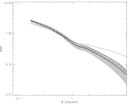
Figure 10: Thick solid and dot-dashed lines: $\xi_{\nu=2}$ of the input model and estimator when the noise is homogeneous, as in Fig. (1). When the noise is inhomogeneous, the thin solid line gives $\xi_{\nu=2}$ obtained when we apply the same method as if the noise were homogeneous. The long-dashed line corresponds to the case when we take into account the variable amplitude of the noise and select pixels accordingly (see text). The shaded area is the 1-sigma optimal variance error bars.

4.2.3 Results

We performed 150 simulations of WMAP data using the SCDM model, with inhomogeneous noise and foreground residuals. We choose three different galactic cuts and two different amplitudes for the foreground residuals: 10% and 20% amplitude of the original foreground data at 94GHz. In the first case, we performed simulations with a Galactic cut at $|b|=5{{}^{\circ}}$ and $10{{}^{\circ}}$ and for the 20% residuals we imposed a cut at $|b|=20{{}^{\circ}}$. We have checked that these models give a foreground residual level comparable to the actual contribution found in the data by Bennett et al. (2003c).

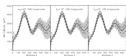
Figure 11: Radiation power spectra obtained from maps containing inhomogeneous noise and foreground residuals. The correlation function was computed using all pixels above $\nu=2$. As in Fig. (4), solid lines correspond to the input power spectrum. The dotted lines give the average of 150 simulations. The dashed lines show the 1-$\sigma$ confidence level given by the optimal variance of Eq. (6). The shaded area corresponds to the 1-$\sigma$ error region obtained from the simulations.

In Fig. (11) we show the results of 150 simulations. As in Fig. (4), the dotted lines shows the mean power spectrum of all the simulations, while the solid line shows the input model. Shaded areas give the 1-$\sigma$ confidence level and dashed lines the optimal variance 1-$\sigma$ error bars (see Eq. (6)). In the whole range, the error bars were almost identical (less than 5% increase) to the case with no foregrounds and homogeneous noise. The correlations in $l$-space are practically the same as before ($\Delta l\simeq 10$). The deviations of the mean from the input model are from the smaller number of simulations.

To quantify the amplitude of the non-Gaussian components, we computed the skewness and kurtosis of our simulations. The skewness and kurtosis are defined (cf. Press et al. 1992) as $\sigma_{3}=\langle(\delta T/\sigma_{2})^{3}\rangle$, $\sigma_{4}=\langle(\delta T/\sigma_{2})^{4}\rangle-3$, respectively, with $\sigma_{2}$ being the variance of the data. In our case, the non-gaussian signal is dominated by the foreground residuals. We computed the skewness and kurtosis for a randomly selected map of the previous set of simulations. For a Galactic cut at $10{{}^{\circ}}$ and 10% foreground residuals amplitude, the values found were $\sigma_{3}=0.12$ and $\sigma_{4}=1.2$. For comparison, for the same CMB map re-simulated with a realistic noise component, galactic cut and no foregrounds, the values were $\sigma_{3}=0.02$ and $\sigma_{4}=-0.03$.

To conclude, the addition of a non-Gaussian signal (the foreground residuals) and inhomogeneous noise does not affect significantly the performance of the method. The reason that the introduction of Galactic foregrounds produces only small variations in the results is at the very core of our procedure: with the new KHA statistic, Eq. 3 we select regions with high S/N ratio, the peaks, and small departures from gaussianity neither degrades the quality of our subset of data, nor introduces additional correlations.

The results presented in Fig. (11) would improve for lower thresholds. As the method provides correlated $C_{l}$’s, it is necessary to bin the estimates into band powers. Other methods share, to some extent, this limitation; direct computation of the power spectrum from a map which necessarily has a cut due to bright foreground regions, is possible only with a finite band-width determined by size of the Galactic cut. This was avoided in the COBE/DMR data with the Gramm-Schmidt orthogonalization of the base functions (Górski 1994), but the procedure is impractical for the mega-pixel CMB datasets. For the WMAP 94 GHz channel, our method provides, under reasonable accuracy, around 12-14 independent data points for the first two Doppler peaks of the CMB power spectrum, and with a gain factor of $10^{3}-10^{4}$ in CPU time compared to standard methods.

We have also demonstrated that our method retains its accuracy in the presence of foregrounds and for the realistic/inhomogeneous WMAP noise. The treatment in the presence of the inhomogeneous noise can also be improved by removing the pixels with significantly fewer observations. Furthermore, because the peaks method computes a correlation function, $\xi_{\nu}$, it is immune to masking. The latter would allow us to reduce the foregrounds signal by removing from the CMB maps more isolated regions with higher foreground contribution.

5 Application to Planck

The Planck satellite is due to be launched in early 2007 to map the all sky CMB distribution with an even finer resolution than WMAP. It will have two instruments: the low-frequency instrument (LFI), that operates at three frequency channels between 30 and 70 GHz, and the high-frequency instrument (HFI) in six frequency channels between 100 and 857 GHz. The highest Planck resolution will be 5 arcmin and the instrument noise after one year of operations is expected to be around 6-10 $\mu$K.

For this case we simulated the 217 GHz channel, with a beam of $5.5^{\prime}$ FWHM and an average noise level of $11.4{\rm\mu}$K per beam area. We tested this channel in two different cosmological models: for consistency, we performed 125 simulations with the same SCDM model used for WMAP, (top row of Fig. (12), but we also tested our method with the $\Lambda$CDM concordance model, given by $\Omega_{\rm m}=0.292$, $\Omega_{\Lambda}=0.708$, $\Omega_{\rm b}=0.044$ and $h=0.72$, (bottom row of the same figure). We assumed that the instrumental noise was the sum of two different components with white noise and $1/f$ contributions (see Maino et al. 1999 for a detailed account of systematic effect on the Planck LFI instrument).

The $1/f$ component is characterized by a knee frequency $f_{k}$, for which the power spectra of both white and $1/f$ noise components are equal. If the spin frequency $f_{s}$ is not much smaller than the knee frequency $f_{k}$, then we can use the fact that the telescope spends sixty minutes in each ring to simply consider the average noise pattern for every ring, (Maino et al. 2002). In other words, we can neglect the noise high frequency components present in the same ring, as these will be averaged out. We model the $1/f$ component as a different baseline present in every scanned ring, giving a pattern of stripes in the noise map (Janssen et al. 1996). We used the Planck 217 GHz channel noise model, provided to us by the Max Planck Institute für Astrophysik (MPA) at Garching, that includes all systematic effects. For each simulation, we added a realization of this $1/f$ component to the cosmological and white noise components. For simplicity we did not include foreground residuals as in the previous section we have shown to give negligible contribution. For similar reasons we also did not include point sources.

The maximum multipole to which a beam of $5.5^{\prime}$ FWHM is sensitive is $l_{\rm beam}=1472$. The HEALPix configuration chosen to pixelize the CMB sky as seen by this channel was $N_{\rm side}=1024$, which yields pixels of 3.5 arcmins. In Fig. (12) we show the results of 500 simulations. As indicated, we have chosen three threshold levels that have the same number of pixels that the three $\nu$’s considered for WMAP. We plot the results for those thresholds following the conventions of Fig. (4). Note that, while we obtain the radiation power spectrum from the same number of pixels as in the case of WMAP, the method recovers it up to $l=1472$, the largest possible multipole determined by the beam size. This could be expected, since the clustering of peaks and troughs is a statistic particularly sensitive to small angular scales. In the range $\theta\in[\theta_{\rm beam},\sim 10^{0}]$, or equivalently $l\in[40,l_{\rm beam}]$, our method reconstructs the power spectrum with an accuracy depending only on the threshold. The range in $l$-space probed by the method depends on the resolution of each experiment but is independent of the total number of peaks used in the analysis.

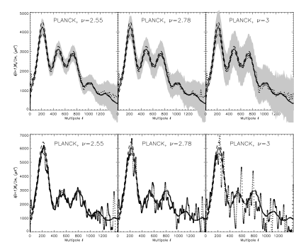
Figure 12: Radiation power spectrum for the Planck 217 GHz channel: in the top row we have considered the SCDM model used in WMAP simulations. In the top panels we follow the conventions of Fig. (4): solid lines represent the input model, dotted lines the mean of 125 simulations, dashed lines are optimal variance error bars at $1\sigma$ and the shaded areas are the same confidence limit obtained from the simulations. In the bottom row, we show results for the concordance $\Lambda$CDM model for one single realization (dotted line). Again, the input model is given by the solid line and the optimal variance error bars are given, as before, by the dashed lines.

Using the data from the three set of simulations we can compute how the band power error bars scale with the threshold $\nu$. In this case, a fit of the form $\sigma_{C_{l}}\propto N_{\rm peaks}^{\beta}$ to the error bars of all multipoles gives: $\beta=-0.65\pm 0.011$, close to the expected behavior $\sigma_{C_{l}}\propto 1/\sqrt{N_{\rm peaks}}$. As mentioned before, this scaling can be used to decide what threshold to choose to achieve a preselected accuracy. The correlations on the $C_{l}$’s were similar to those of WMAP, of the order of $\Delta l\simeq 10$.

6 Discussion and conclusions

We have presented the detailed implementation of the peaks KHA method for computing the CMB power spectrum. The method is based on the correlation properties of peaks on the CMB and assumes that temperature fluctuations are Gaussian. We have shown, that the method is robust in the presence of Galactic (non-Gaussian) foregrounds and realistic WMAP and Planck noise inhomogeneities.

This method provides a new and independent way to characterize the sub-degree structure of the CMB. Its accuracy is generally lower than standard methods, but it is remarkably faster for the range of values of $\nu$ required by WMAP and Planck. This is demonstrated in Fig. (13), where we compare speed of a standard ${\cal O}$(N log N) $\sim\leavevmode\nobreak\ N^{1.61}$ method with ours.

Figure 13: The value of the peak threshold where the number of operations in the KHA method equals $N^{1.61}$, is plotted as a function of the number of pixels.

For WMAP the KHA method should work most optimally for peak thresholds of $\nu\sim 1.8-2.5$ or in only $(2.5\times 10^{-3}-8\times 10^{-5})N^{2}$ operations. Applying the method to the simulated PLANCK sky maps has shown that we could probe, with the same number of points, the power spectrum out to much higher multipoles and without significant loss of accuracy. For Planck mission parameters, the KHA method should work most optimally for $\nu\sim 2-3$, reducing the number of steps down to $\sim 4\times 10^{-6}N^{2}$ operations for thresholds as high as $\nu\sim 3$. This can potentially lead to a gain of up to $\sim 10^{5}$ in speed compared to the existing O$(N^{2})$ methods.

A significant advantage is that because we use a $\xi_{\nu}$ statistic, the computed CMB spectrum is immune to masking, allowing to remove high noise and foreground emission parts of the sky. This also makes straightforward the analysis of particular isolated regions in the sky, enabling its application to future CMB experiments of very high angular resolution scanning small celestial patches.

With the scalings of $\sigma_{C_{l}}$ with $\nu$ for both WMAP and Planck one can estimate the uncertainties of the different multipoles at still lower peak threshold values. In Fig. (14) we show what would be the spectrum recovered from the 2 year WMAP data release using a threshold $\nu=1.6$. The whole calculation would require only $6\times 10^{-3}N^{2}$ operations.

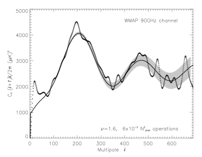
Figure 14: Radiation power spectrum that would be recovered using the WMAP second year data with a threshold of $\nu=1.6$: it was obtained in only $6\times 10^{-3}N^{2}$ operations. The solid line corresponds to the input model and the dotted line is the raw power spectrum recovered from one single simulation, prior to binning. The shaded area shows the extrapolated 1-$\sigma$ uncertainties of the CMB power spectrum binned with $\Delta l=45$.

REFERENCES
Bardeen, J.M., Bond, J.R., Kaiser, N. & Szalay, A.S. 1986, ApJ, 304, 15
Bennett, C., Halpern, M., Hinshaw, G. et al. 2003a, ApJ, accepted
Bennett, C., Hill, R.S., Hinshaw, G. et al. 2003b, ApJ, accepted
Bond, J.R., Jaffe, A.H. & Knox, L. 2000, ApJ, 533, 19.
Finkbeiner, D.P., Davis, M., Schlegel 1999, ApJ, 524, 867
Górski, K.M. 1994, ApJ 430, L85
Górski, K.M, Hivon, E. & Wandelt, B.D., 1999, Proceedings of the MPA/ESO Cosmology Conference ”Evolution of the Large Scale Structure”, eds. A.J.Banday, R.S.Sheth and L.Da Costa, PrintPartners Ipskamp, NL, pp.37-42.
Hinshaw, G. 2000, Proceedings of the MPA/ESO/MPE Workshop “Mining the Sky”, held at Garching, Germany, 31st July - 4th August 2000. Edited by A.J.Banday, S.Zaroubi and M.Bartelmann. Heidelberg: Springer-Verlag, 2001, p.447
Hivon, E., Górski, K.M, Netterfield, C.B. et al. 2002 ApJ, 567, 2
Hu, W. & Dodelson, S. 2002, A.R.A.A., 40, 171
Janssen, M., Scott, D., White, M. et al. 1996, astro-ph/9602009
Jarosik, N., Bennett, C.L., Halpern, M. et al., 2003, ApJS, 145, 413
Jensen, L.G. & Szalay, A.S. 1986 ApJ, 305, L5
Kaiser, N. 1984 ApJ, 282, L9
Kashlinsky, A. 1987, ApJ 317, 19
Kashlinsky, A., Hernández-Monteagudo, C. & Atrio-Barandela, F. 2001 ApJ, 557, L1 (KHA)
Knox, L., 1995, Phys. Rev. D, 52, 4307
Kogut, A., Banday, A.J., Bennett, C.L. et al. 1996, ApJ, 464, L5
Landy, S.D & Szalay, A.D. 1993 ApJ 412, 64
Maino, D., Burinaga, C., Maltoni, M. et al. 1999, A&AS, 140, 383
Maino, D., Burinaga, C., Górski, K.M, Mandolesi, N. & Bersanelli, M. 2002, A&A, 387, 356
Oh, S.P., Spergel, D.N. & Hinshaw, G. 1999 ApJ, 510, 551
Padmanabhan, N., Seljak, U. & Penn, U.L. 2003 NewA 8 581
Page, L., Nolta, N.R, Barnes, C. et al., 2003, ApJ, accepted
Peebles, P.J.E. 1980 “The Large Scale Structure of the Universe”, Princeton University Press, Princeton
Penn, U., 2003, astro-ph/0304513
Press, W.H., Teukolsky, S.A., Vetterling, W.T. & Flannery, B.P. 1992 “Numerical Recipes”, 2nd edition, Cambridge University Press, Cambridge
Rice, S.O. 1954, in “Noise and Stochastic Processes”, ed. Wax, N., p.133 Dover (NY)
Seljak, U. & Zaldarriaga, M. 1996, Ap. J., 469, 437 Smoot, G.F., Bennett, C.L., Kogut, A. et al. 1992, ApJ, 396, L1
Sokasian, A., Gawiser, E. & Smoot G.F. 2001, ApJ 562 885
Szapudi, I., Prunet, S., Pogosyan, D. et al 2001, ApJ, 548, L115
Szapudi, I., Prunet, S. & Colombi, S. 2001, ApJ, 561, L11
Schlegel, D.J., Finkbeiner, D.P. & Davis, M. 1998, ApJ, 500, 525
Tegmark, M. 1997, Phys.Rev.D., 55, 5898
Wandelt, B.D., Hivon, E. & Górski, K. 2001, Phys.Rev.D, 64, 083003