Using Supernovae to Determine the Equation of State of the Dark Energy:
Is Shallow Better Than Deep?

Abstract

Measurements of the flux and redshifts of Type Ia supernovae have provided persuasive evidence that the expansion of the universe is accelerating. If true, then in the context of standard FRW cosmology this suggests that the energy density of the universe is dominated by “dark energy” – a component with negative pressure of magnitude comparable to its energy density. To further investigate this phenomenon, more extensive surveys of supernovae are being planned. Given the likely timescales for completion, by the time data from these surveys are available some important cosmological parameters will be known to high precision from CMB measurements. Here we consider the impact of that foreknowledge on the design of supernova surveys. In particular we show that, despite greater opportunities to multiplex, purely from the point of view of statistical errors, a deep survey may not obviously be better than a shallow one.

CWRU-P5-02

I Introduction

Over the past few years, measurements of the flux and redshifts of Type Ia supernova have provided increasingly persuasive evidence that the expansion of the universe is accelerating SNCP ; HRSS . The natural inference – that the energy density of the universe is dominated by some form of vacuum energy – has important consequences for both cosmology and particle physics. Of particular interest is the exact nature of the “dark energy.” Is it the so-called cosmological constant, the energy density of the true vacuum state of the universe? Is it predominantly the potential energy density of a new form of energy often called quintessence? or is it something else entirely? Since these each have dramatic, and dramatically different, implications for fundamental physics there is a clear need both to raise the confidence level of the conclusion that the expansion is accelerating, and to better characterize the time history of that expansion so that the nature of the “dark energy,” in particular its equation of state, can be better understood.

II CMB As a Probe of Cosmological Parameters

The recent expansion history of the universe (after matter-radiation equality) – the evolution of the scale factor $a$ with time $t$, or with conformal time $\eta$ ($dt=a(\eta)d\eta$) – is given by the Friedman equation:

$$\frac{da}{d\eta}\!=\!\sqrt{\Omega_{o}\!H_{o}^{\!2}\!}\sqrt{\frac{a}{a_{o}}\!+\!\frac{\Omega_{c}}{\Omega_{o}}\!\left(\!\frac{a}{a_{o}}\!\right)^{\!2\!}\!+\!\frac{1\!-\!\Omega_{o}\!-\!\Omega_{c}}{\Omega_{o}}\!\left(\!\frac{a}{a_{o}}\!\right)^{\!(\!1\!-\!3\!w\!)\!}}.$$ (1)

The evolution of the expansion is therefore characterized by $\Omega_{o}$, the current ratio of the matter energy density to the critical energy density, $\Omega_{c}$, the current ratio of the curvature “energy density” to the critical energy density, $H_{o}$, the current value of the Hubble parameter, and $w$ the equation of state parameter for the dark energy. ($p_{dark}=w\rho_{dark}$.)

Great success has already been achieved in determining some of these parameters by a number of techniques, and even greater precision is likely in the near future. We will focus in particular on measurements of temperature anisotropies in the cosmic microwave background radiation (CMB). The positions of the acoustic peaks in the angular power spectrum of the CMB depend on $\eta_{ls}$ (the conformal lookback time to the last-scattering surface) and on the geometry of the universe, parametrized by $\Omega_{c}$. The shapes of the peaks depend sensitively on $\Omega_{o}h_{o}^{2}$. Current data on the first three peaks Boomerang ; MAXIMA ; DASI already argue strongly for a flat (or nearly flat) universe ($\Omega_{\rm curvature}\simeq 0$). With anticipated data from the MAP satellite (and elsewhere) the shape of the spectrum should also be well measured. Thus the positions and shapes of the first peaks in the CMB spectrum will soon be used to confine models of the dark energy to a one-dimensional surface parametrized by $w$ parameters . Extracting $w$ from CMBR measurements is far more difficult – the value of $w$ has too little effect on the power spectrum of the anisotropies.

III Supernovae as Standard Candles

While the absolute luminosity of supernovae is not known, properly calibrated Type Ia supernovae seem to be excellent standard candles HRSS ; SNCP . Measurements of the flux and redshift from a distant supernova when compared to measurements of similar supernovae at low redshift ($z_{\rm low}\ll 1$) measures the square of the ratio of the luminosity distances $d_{L}=\eta(1+z)$ as a function of $z$:

$$\frac{F(z,w)}{F(z_{\rm low},w)}=\left[\frac{\eta(z)(1+z)}{\eta(z_{\rm low})(1+z_{\rm low})}\right]^{-2}$$ (2)

It has already been possible, by measuring $\eta(z)$ from the ground for a reasonable sample of supernovae, to argue convincingly that $w<0$ for a significant fraction of the energy density of the universe HRSS ; SNCP .

IV Optimum Survey Strategies for Measuring $w$

Accepting the desirability of improving the determination of $w$ (and perhaps more generally $w(z)$), and working with the assumption that Type Ia supernovae remain the best existing standard candles, one can still ask what is the optimum possible survey strategy? The answer depends very much on the precise goals of the survey previous . One option is to seek independent confirmation of the pre-existing determinations of $\Omega H_{o}^{2}$ and $\Omega_{c}$ while simultaneously measuring $w$ and possibly its derivatives. Alternatively, one could accept the pre-existing measurements of $\Omega H_{o}^{2}$ and $\Omega_{c}$ and confine one’s time and attention to the best possible measurement of $w$ itself. Admittedly, there are clear benefits to independent measurements of cosmological parameters. Nevertheless, we would argue that the uncertainty in the theoretical models of supernovae, coupled with likely observational uncertainties make future supernova surveys less powerful as opportunities for independent checks on existing and near-term CMB-based determinations of parameters than they are as opportunities to break parameter degeneracies that the CMBR measurements cannot or cannot easily break and thus determine quantities like $w$.

The implications of this choice of survey strategies may be significant. From a purely statistical viewpoint, a supernova survey designed to measure $\Omega H_{o}^{2}$, $\Omega_{c}$ and $w$ will necessarily extend to higher z, because it must measure the expansion history over a wide range of $z$ in order to make independent determinations of all three parameters characterizing the evolution of the scale factor. However, except to address issues of systematic effects, a survey designed to measure $w$ only, may not need to extend to such a high redshift, since it seeks to measure only one parameter. We shall therefore pursue this option further.

Assuming perfect knowledge of the CMBR, we can fix the value of $\Omega_{o}H_{0}^{2}$ and $\Omega_{c}$, and of the function $\Omega(w)$. The former two are obtained from a direct fit to the CMB angular power spectrum, while $\Omega(w)$ is obtained as follows. For the purposes of illustration, we shall take $\Omega_{c}=0$. The conformal distance to the surface of last scatter is then

$$\eta_{ls}\simeq\frac{1}{\sqrt{\Omega_{o}H_{o}^{2}}}\int_{0}^{1}\frac{dx}{\sqrt{x+\frac{1-\Omega_{o}}{\Omega_{o}}x^{1-3w}}}\ ,$$ (3)

(where we have taken $a_{ls}\simeq 0$). Fixing $\eta_{ls}$, this can be solved numerically for $\Omega_{o}(w)$; however, a linear fit can be obtained in the neighborhood of any $w$ as follows. Differentiating with respect to $\Omega_{o}$, holding $\Omega_{o}H_{o}^{2}$ and $w$ fixed,

$$\frac{\partial\eta_{ls}}{\partial\Omega_{o}}\Bigr{|}_{\Omega_{o}H_{o}^{2},w}\simeq\frac{1}{\sqrt{\Omega_{o}H_{o}^{2}}}\frac{1}{2\Omega_{o}^{2}}\int_{0}^{1}\frac{x^{1-3w}dx}{\left[x+\frac{1-\Omega_{o}}{\Omega_{o}}x^{1-3w}\right]^{3/2}}\ .$$ (4)

Similarly, differentiating with respect to $w$, holding $\Omega_{o}H_{o}^{2}$ and $\Omega_{o}$ fixed,

$$\frac{\partial\eta_{ls}}{\partial w}\Bigr{|}_{\Omega_{o}H_{o}^{2},w}\simeq\frac{1}{\sqrt{\Omega_{o}H_{o}^{2}}}\frac{3(1-\Omega_{o})}{2\Omega_{o}}\int_{0}^{1}\frac{x^{1-3w}\ln(x)dx}{\left[x+\frac{1-\Omega_{o}}{\Omega_{o}}x^{1-3w}\right]^{3/2}}\ .$$ (5)

Evaluating the ratio of these quantities at, for example, $\Omega_{o}=0.3$, $w=-1$, we find

$$\Omega_{o}(w)\simeq 0.3+0.274(w+1)\ .$$ (6)

Now, given measurements of the flux ratio $F(z,w)/F(z_{\rm low},w)$ between distant supernovae and a sample of low redshift supernova, we can determine $w$. The uncertainty in the determination of $w$ from one measurement of $F(z)/F(z_{\rm low})$ is

$$\sigma_{w}=\left[\frac{d\ln(F/F_{low})}{dw}\right]^{-1}_{\Omega_{o}H_{o}^{2},\Omega(w)}\frac{\sigma_{(F/F_{low})}}{F/F_{low}}$$ (7)

Using the relationship (2), and assuming that any variance is dominated by the uncertainty in the flux determination (i.e. the uncertainty in the redshift is negligible), we can relate $\sigma_{w}$ to $\eta$. For each measurement

$$\sigma_{w}=\frac{1}{2}\frac{\sigma_{(F/F_{low})}/\left(F/F_{low}\right)}{\left|\frac{\partial\ln\eta}{\partial w}-\frac{\partial\ln\eta_{\rm low}}{\partial w}\right|}.$$ (8)

For a survey with a fixed observing time, $\sigma_{w}$ is reduced by the square root of the number of supernovae $N_{SN}$ which can be probed, so that

$$\sigma_{w}^{(survey)}=\frac{\sigma_{(F/F_{low})}/\left(F/F_{low}\right)}{\left|\frac{\partial\ln\eta}{\partial w}-\frac{\partial\ln\eta_{\rm low}}{\partial w}\right|}.\frac{1}{\sqrt{N_{SN}}}\ .$$ (9)

Here we begin to see the impact of alternative observing strategies. For a simple survey with a simple instrument, the number of supernovae which one can observe at a given redshift will be proportional simply to the ratio of the flux of a supernova at the redshift to a fixed threshold flux – $N_{SN}\propto F/F_{thresh}$. However, it is possible to improve on this strategy, especially at high redshifts, by increasing the field of view of the survey instrument, monitoring more than one galaxy at a time for supernovae, and possibly following up with spectra in a fully multi-plexed program. In this case the number of supernova discovered will scale as

$$N_{SN}\propto F~{}\eta^{2}\Delta\eta\propto(1+z)^{-2}\ .$$ (10)

We have taken $\Delta\eta$ – the range in conformal depth of the survey – to be a constant. Other assumptions are possible. While they change the detailed dependence of the statistical errors on redshift, they do not change the qualitative behavior.

For a fully multiplexed survey

$$\sigma_{w}^{(survey)}\propto\frac{\sigma_{(F/F_{low})}/(F/F_{low})}{\left|\frac{\partial\ln\eta}{\partial w}-\frac{\partial\ln\eta_{\rm low}}{\partial w}\right|_{\Omega_{o}H_{o}^{2},\Omega(w)}}(1+z)\ .$$ (11)

Now, in the neighborhood of $w=-1$,

$$\eta|_{\Omega_{o}H_{o}^{2}}\simeq\frac{1}{\sqrt{\Omega_{o}H_{o}^{2}}}\int_{1/(1+z)}^{1}\frac{dx}{\sqrt{x+\frac{7}{3}x^{4}}}$$ (12)

and

$$\left(\frac{d\eta}{dw}\right)_{\Omega_{o}H_{o}^{2}}\simeq\frac{1}{2\sqrt{\Omega_{o}H_{o}^{2}}}\times$$ (13)

$$\times\int_{1/(1+z)}^{1}\frac{x^{4}dx}{\left(x+\frac{7}{3}x^{4}\right)^{3/2}} \left(7\ln(x)+\frac{0.274}{(0.3)^{2}}\right)\ .$$ (14)

These integrals can be evaluated numerically without difficulty, allowing us to calculate $\sigma_{w}^{(survey)}$ as a function of the redshift of the observations for a variety of $w$’s (cf. Fig. 1). The principal point of interest is that while $\sigma_{w}^{(survey)}$ has a minimum at $z\simeq 1$ (somewhat lower for $w<-1$, somewhat higher for $w>-1$), this minimum is exceedingly shallow, so that the value of $\sigma_{w}$ at $z=0.3$ is less than twice the minimum value. Moreover, our calculations involved the supernova discovery rate. However, it is in fact the follow up spectroscopy which is more demanding of telescope time; this scales as a higher power of redshift (approximately $(1+z)^{6}$ according to some experts). This shifts the minimum down further in $z$. These results are relatively insensitive to the value of $w$, and to reasonable values of $z_{\rm low}$.

We have thus shown that, from a statistical point of view, there is not the strong preference one might have suspected to measure $w$ at high redshift – intermediate redshifts ($z=0.3-0.5$) are nearly as good for discovering supernovae, and at least as good for carefully studying them. The length of time that one must integrate on individual distant supernovae offsets the benefits one might get from the greater individual utility of these supernova and the larger accessible number of such supernova. The details of the survey statistics will no doubt change as one designs a more realistic survey, but the broad conclusion will not – for measuring $w$ with supernova, statistics are as good or better at low $z$ than at high $z$. The low z surveys offer the advantage of smaller K corrections and the ability to study the host galaxy properties in detail with a wide array of ground based telescopes. For the low z surveys to be competitive with the high z surveys, they require even more exquisite control of systematic photometric errors. Ultimately, detailed trade studies are needed to determine the best strategy for determining the properties of the dark energy. These studies should include our growing knowledge about the geometry and composition of the universe in their analyses.

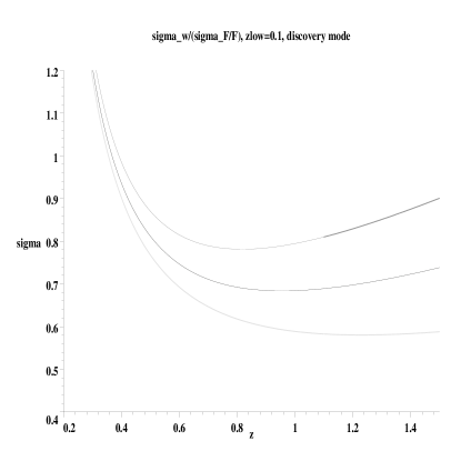
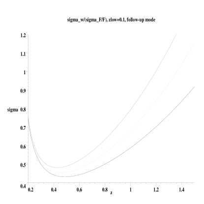
Figure 1: The statistical error, $\sigma$, in the determination of $w$ from a survey of fixed duration conducted in a narrow range of redshifts around some redshift z, plotted as a function of that redshift. The plots are in arbitrary units for $w=-1$, and $z_{low}=0.1$. The left hand plot is for “discovery mode”($N\propto(1+z)^{-2}$); the right hand plot is for “follow up mode”($N\propto(1+z)^{-6}$). In each, curves are for $w=-1.3$ (top), $w=-1$ (middle) and $w=-0.6$ (bottom).

GDS would like to acknowledge fruitful discussions with J. Freeman, D. Huterer, E. Linder, S. Perlmutter, and M. Turner. Particular thanks to M. Turner for pointing out a sign error in an earlier version as well as other useful comments.

References

- (1) S. Perlmutter et al, Astrophys.J. 517, 565 (1999).
- (2) A.G. Riess et. al. Astron. J. 116, 1009-1038 (1998); P. M. Garnavich et al., Ap. J. 493, L53-57k (1998).
- (3) C.B. Netterfield, P.A.R. Ade, J.J. Bock, J.R. Bond, J. Borrill, A. Boscaleri, K. Coble, C.R. Contaldi, B.P. Crill, P. de Bernardis, P. Farese, K. Ganga, M. Giacometti, E. Hivon, V.V. Hristov, A. Iacoangeli, A.H. Jaffe, W.C. Jones, A.E. Lange, L. Martinis, S. Masi, P. Mason, P.D. Mauskopf, A. Melchiorri, T. Montroy, E. Pascale, F. Piacentini, D. Pogosyan, F. Pongetti, S. Prunet, G. Romeo, J.E. Ruhl, F. Scaramuzzi astro-ph/0104460.
- (4) R. Stompor , M. Abroe, P. Ade, A. Balbi, D. Barbosa, J. Bock, J. Borrill, A. Boscaleri, P. De Bernardis, P.G. Ferreira, S. Hanany, V. Hristov, A.H. Jaffe, A.T. Lee, E. Pascale, B. Rabii, P.L. Richards, G.F. Smoot, C.D. Winant, J.H.P. Wu, Astrophys.J. 561 (2001) L7-L10.
- (5) E. M. Leitch, C. Pryke, N. W. Halverson, J. Kovac, G. Davidson, S. LaRoque, E. Schartman, J. Yamasaki, J. E. Carlstrom, W. L. Holzapfel, M. Dragovan, J. K. Cartwright, B. S. Mason, S. Padin, T. J. Pearson, M. C. Shepherd, A. C. S. Readhead astro-ph/0104488; N. W. Halverson, E. M. Leitch, C. Pryke, J. Kovac, J. E. Carlstrom, W. L. Holzapfel, M. Dragovan, J. K. Cartwright, B. S. Mason, S. Padin, T. J. Pearson, M. C. Shepherd, A. C. S. Readhead astro-ph/0104489; C. Pryke, N. W. Halverson, E. M. Leitch, J. Kovac, J. E. Carlstrom, W. L. Holzapfel, M. Dragovan astro-ph/0104490.
- (6) Recent reviews include: M. Kamionkowsky and A. Kosowsky, Ann. Rev. Nucl. Part. Sci. 49 77 (1999) and W. Hu and S. Dodelson, Ann. Rev. Astron. Astrophys. in press (2002). For expectations from analysis of MAP data see, most recently A. Kosowsky, M. Milosavljevic, R. Jimenez, astro-ph/0206014.
- (7) Previous work on the design of supernova surveys for cosmology includes most recently D. Huterer, M. Turner, Phys. Rev. D, 64, 123527 (2001); also M. Goliath, R. Amanullah, P. Astier, A. Goobar, R. Pain astro-ph/0104009; E. Linder, astro-ph/0108280; D.J. Eisenstein, W. Hu, M. Tegmark astro-ph/9805239; W. Hu, D.J. Eisenstein, M. Tegmark, M. White Phys.Rev. D59 (1999) 023512.