When can preheating affect the CMB?

Abstract

We discuss the principles governing the selection of inflationary models for which preheating can affect the CMB. This is a (fairly small) subset of those models which have non-negligible entropy/isocurvature perturbations on large scales during inflation. We study new models which belong to this class - two-field inflation with negative nonminimal coupling and hybrid/double/supernatural inflation models where the tachyonic growth of entropy perturbations can lead to the variation of the curvature perturbation, ${\cal R}$, on super-Hubble scales. Finally we present evidence against recent claims for the variation of ${\cal R}$ in the absence of substantial super-Hubble entropy perturbations.

]

I Introduction

The cosmological landscape is now dominated by a myriad of inflationary models [1], each with slightly different genetics but a common origin, forged in the heyday of Grand Unified field theories [2]. Inflationary models are flexible, hardy and spawn & multiply with remarkable facility - features flowing from their scalar field DNA.

And while the recent M-theory and brane-world revolution has again stimulated interest in alternatives to inflation [3] it remains true that the simplest inflationary models provide a very good fit to current cosmological observations [4]. Indeed, the Cosmic Microwave Background (CMB) and large scale structure observations presently show no particular signature - such as primordial non-Gaussianity - which might allow us to single out a particular model or falsify inflation as a paradigm. It is therefore good science to seek new ways to select the “fittest” of inflationary models.

Preheating after inflation may provide exactly such a selection rule. Preheating is probably the most violent of putative phases in cosmic history [5, 6]. It requires non-perturbative quantum field theory pushed to its non-equilibrium limits [7]. The exponentially rapid population of sub- and super-Hubble wavelength modes makes it possible to produce very massive particles in large quantities and hence over-produce dangerous relics such as modulini or gravitini [8]. In addition there is some (admittedly speculative) evidence that the induced parametric growth of small-wavelength metric perturbations around the Hubble scale may lead generically to runaway production of primordial black holes (PHB) [9]. If correct this will rule out wide regions of the preheating parameter space.

At the other end of the cosmic scale, a natural question is whether preheating can affect the modes of the metric perturbations which induce the intricate anisotropies in the CMB, and if so, what are the criteria? In this paper we will discuss the conditions where preheating can lead to the growth of metric perturbations on cosmic scales.

The answer to this question appears to be intimately linked to the issue of correlations between adiabatic and entropy perturbations from multi-field inflation.

II General principles

In this section we present the conditions known to be sufficient for preheating to affect the CMB; distilled from the recent literature [10]-[21]. Perhaps the best way to discuss the impact on the CMB is via quantities which are time-independent in the presence of only adiabatic perturbations on large scales. Such quantities are used to normalize the inflationary models to the large-angle COBE measurements of the CMB.

Two common choices for such quantities are $\zeta$, the curvature perturbation in the constant density hypersurfaces ($\delta\rho=0$), and the comoving curvature perturbation ${\cal R}$. These two coincide in the $k\to 0$ limit [22] (modulo a minus sign) and we will use ${\cal R}$.

The existence of entropy perturbations is crucial for preheating to affect the CMB, since in general [23]

$$\dot{{\cal R}}\rightarrow 3H\frac{\dot{p}}{\dot{\rho}}{\cal S}\,,$$ (1)

where the above limit is understood as $k\rightarrow 0$; $H$, $p,\rho$ are the Hubble rate, the total pressure and energy density respectively and ${\cal S}$ is the total (dimensionless) entropy perturbation defined by

$${\cal S}=H\left(\frac{\delta p}{\dot{p}}-\frac{\delta\rho}{\dot{\rho}}\right)\,.$$ (2)

Now in the case of two minimally coupled scalar fields $\varphi_{1}$ and $\varphi_{2}$, this can be given explicitly [22] as

$$\dot{{\cal R}}\rightarrow\frac{2H}{\dot{\sigma}}\dot{\theta}\delta s.$$ (3)

where $\sigma$ and $s$ are “adiabatic” and “entropy” fields, defined by

$$d\sigma = (\cos\theta)d\varphi_{1}+(\sin\theta)d\varphi_{2},$$ (4)

$$ds = -(\sin\theta)d\varphi_{1}+(\cos\theta)d\varphi_{2}\,.$$ (5)

Here $\theta$ is the angle of the trajectory in $(\phi,\chi)$ field space, satisfying $\tan\theta=\dot{\varphi}_{2}/\dot{\varphi}_{1}$. Eq. (3) means that variation of ${\cal R}$ requires not only a large scale entropy perturbation $\delta s$, but also a non-straight trajectory in field space. In the minimally coupled two-field system with an effective potential $V(\varphi_{1},\varphi_{2})$, the Fourier modes for the adiabatic and entropy field perturbations satisfy [22]

$$\delta\ddot{\sigma}+3H\delta\dot{\sigma}+\left(\frac{k^{2}}{a^{2}}+V_{\sigma\sigma}-\dot{\theta}^{2}\right)\delta\sigma$$ (6)

$$= -2V_{\sigma}\Phi+4\dot{\sigma}\dot{\Phi}+2(\dot{\theta}\delta s)^{\cdot}-\frac{2V_{\sigma}}{\dot{\sigma}}\dot{\theta}\delta s,$$ (7)

$$\delta\ddot{s}+3H\delta\dot{s}+\left(\frac{k^{2}}{a^{2}}+V_{ss}+3\dot{\theta}^{2}\right)\delta s=\frac{\dot{\theta}}{\dot{\sigma}}\frac{k^{2}}{2\pi Ga^{2}}\Phi,$$ (8)

where $k$ is a comoving momentum, $a$ is a scale factor, $G$ is a Newton’s gravitational constant, and

$$V_{\sigma\sigma} \equiv (\cos^{2}\theta)V_{\varphi_{1}\varphi_{1}}+(\sin 2\theta)V_{\varphi_{1}\varphi_{2}}+(\sin^{2}\theta)V_{\varphi_{2}\varphi_{2}},$$ (9)

$$V_{ss} \equiv (\sin^{2}\theta)V_{\varphi_{1}\varphi_{1}}-(\sin 2\theta)V_{\varphi_{1}\varphi_{2}}+(\cos^{2}\theta)V_{\varphi_{2}\varphi_{2}}.$$ (10)

$\Phi$ is a gravitational potential in the longitudinal gauge, satisfying

$$\dot{\Phi}+H\Phi=4\pi G\dot{\sigma}\delta\sigma.$$ (11)

Eq. (11) indicates that the gravitational potential is sourced by adiabatic field perturbations.

When the effective mass of $\delta s$ is light relative to the Hubble rate $H=\dot{a}/a$ during inflation, i.e.,

$$\mu_{s}^{2}\equiv V_{ss}+3\dot{\theta}^{2}~{}\mbox{\raisebox{-4.30554pt}{$\stackrel{{\scriptstyle\textstyle<}}{{\textstyle\sim}}$}}~{}H^{2}\,,$$ (12)

the entropy field perturbation is not suppressed on super-Hubble scales during inflation. Then during preheating if $\delta s$ is resonantly amplified due to a time-dependent effective mass, this can lead to the growth of ${\cal R}$ on large scales, thereby altering the power spectrum normalization or even leaving the model incompatible with the large-angle CMB. Note that the adiabatic field perturbation is sourced by the entropy field perturbation, thereby stimulating the growth of $\Phi$ through Eq. (11). In contrast, if the entropy perturbation is heavy during inflation, ($\mu_{s}^{2}\gg H^{2}$) then $|\delta s|\sim a^{-3/2}$ and the growth during preheating means that the change of ${\cal R}$ is negligible before backreaction ends the resonance.

In Sec. IV we present new classes of models which have strong preheating or tachyonic growth but simultaneously have a light entropy perturbation in the preceding inflationary phase. To begin with we shall analyze the evolution of ${\cal R}$ in the massive chaotic inflationary scenario in the next section.

III An evaluation of claims for varying ${\cal R}$ in the absence of entropy perturbations

There have been recent claims by Henriques and Moorhouse (HM) [17] that ${\cal R}$ or $\zeta$ will vary during reheating or preheating even in the absence of large-scale entropy perturbations when going beyond linear perturbation theory and taking into account the quantum-to-classical transition.

If correct this would have a profound impact on inflationary cosmology [11, 12, 13]. Our aim in this section is to evaluate these claims. To do so let us consider metric preheating in the massive chaotic inflationary scenario with a standard four-leg interaction:

$$V=\frac{1}{2}m^{2}\phi^{2}+\frac{1}{2}g^{2}\phi^{2}\chi^{2}\,.$$ (13)

Strong amplification of the $\chi$ fluctuation requires a resonance parameter $q=g^{2}\phi^{2}/(4m^{2})\gg 1$ at the beginning of preheating [6]. In this case the field $\chi$ is heavy during inflation relative to the Hubble rate [14], which means that $\chi$ is strongly suppressed during inflation ($\chi\sim a^{-3/2}$), thereby leading to $\dot{\theta}\simeq 0$ and $\langle V_{ss}\rangle\simeq\langle V_{\chi\chi}\rangle\simeq g^{2}\phi^{2}\gg H^{2}$. Therefore large scale entropy perturbations are exponentially suppressed during inflation, which safeguards nonadiabatic growth of super-Hubble curvature perturbations, as found by Eq. (3). Hence, at the linear level, $\dot{\cal R}\simeq 0$ to high precision in this model.

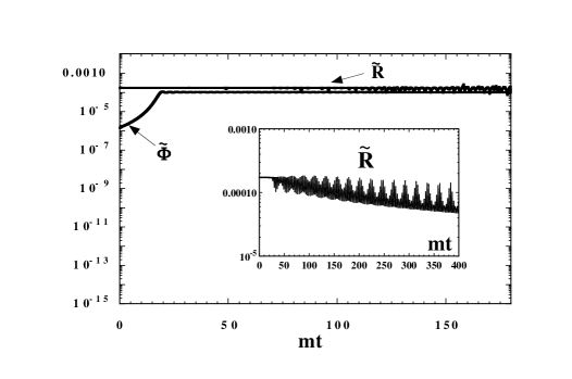
FIG. 1.: The evolution of a super-Hubble curvature perturbation $\tilde{\cal R}\equiv k^{3/2}{\cal R}$ and the gravitational potential $\tilde{\Phi}\equiv k^{3/2}\Phi$ during inflation and preheating in the model (13) with $g=5.0\times 10^{-4}$. The initial conditions are chosen to be $\phi=3M_{\rm pl}$ and $\chi=10^{-3}M_{\rm pl}$, in which case inflation ends around $mt\sim 20$. Inset: The plot of $\tilde{\cal R}$ for large initial variance, $\langle\delta\phi^{2}\rangle=10^{-4}\phi_{0}^{2}$.

Nevertheless we have to caution that $\dot{\cal R}$ in Eq. (3) is the result of the first order perturbation theory. If we include second order backreaction effects in the background evolution equations, these give rise to second order terms such as $\langle\delta\dot{\phi}^{2}\rangle$ in the time derivative of $\dot{\cal R}$ [17]. Since these variances are not suppressed during inflation (due to the short-wavelength contributions), they may provide additional source terms for the curvature perturbation. This, in essence, is the origin of the claims by HM.

To check these claims we performed our numerical simulations implementing the second order backreaction effects as spatial averages in the evolution equations [6, 7, 19, 20] and compared the evolution of the cosmological perturbations found using different (but equivalent at linear order) equations of motion.

In Fig. 1 we plot the evolution of a super-Hubble curvature perturbation using its definition, i.e., ${\cal R}=\Phi-H/\dot{H}(\dot{\Phi}+H\Phi)$. The variance $\langle\delta\chi^{2}\rangle$ grows by parametric resonance until backreaction becomes important, while the inflaton fluctuation is not excited unless rescattering is taken into account [24].

The coherent oscillation of the inflaton condensate is destroyed once backreaction starts to dominate. This can affect the evolution of $H$, $\Phi$ through Eq. (11) and also ${\cal R}$. In fact the curvature perturbations exhibits small oscillations, but it remains roughly constant (see Fig. 1). When we use the first order equation (3), we found that ${\cal R}$ is conserved without oscillations.

This is in stark contrast to the simulations of HM [17] who found that ${\cal R}$ varies after the energy density of the inflaton condensate drops below its variance $\langle\delta\phi^{2}\rangle$. According to their numerical results using similar second order approximations such as ours, the decrease of ${\cal R}$ occurs in the preheating stage.

A large difference between the two investigations is that the initial energy density of the variance $\langle\delta\phi^{2}\rangle$ is smaller than $\phi_{0}^{2}$ only by four orders of magnitude in Ref. [17], while we argue that the typical size is regulated to be $\langle\delta\phi^{2}\rangle\sim m^{2}\sim 10^{-12}M_{\rm pl}^{2}$ [24], which is by ten orders of magnitude smaller than $\phi_{0}^{2}$.

Since $\langle\delta\phi^{2}\rangle$ does not exceed $\phi_{0}^{2}$ during preheating in our simulations, we do not find the decrease of ${\cal R}$ claimed by [17]. Using the initial conditions of HM we checked that curvature perturbations exhibit small decrease after $\phi_{0}^{2}$ drops under $\langle\delta\phi^{2}\rangle$ (see the inset of Fig. 1), but we still do not find the extensive changes reported in [17].

We did find that implementing the numerics is subtle and subject to artificial instabilities. Further, not all definitions or equations for ${\cal R}$ are equally suitable for numerical implementation, some being more susceptible to these instabilities. We therefore argue that ${\cal R}$ probably does not evolve on large scales in the absence of entropy perturbations even at second order. This is consistent with the standard view based on causality .

We end with one caveat, however: full lattice simulations show that the growth of $\delta\chi$ leads to the excitation of inflaton fluctuations via rescattering, thereby satisfying the condition $\langle\delta\phi^{2}\rangle~{}\mbox{\raisebox{-4.30554pt}{$\stackrel{{\scriptstyle\textstyle>}}{{\textstyle\sim}}$}}~{}\phi_{0}^{2}$ around the end of preheating [24]. It would be worth investigating further whether any change in ${\cal R}$ occurs in such a situation, although if they do, they are likely to be small.

IV Models with the CMB affected by preheating

A Chaotic inflation with self-interaction and nonminimal coupling

Achieving a light entropy perturbation during inflation is typically rather difficult in chaotic inflation models. However, this picture is modified if one takes into account nonminimal coupling [16]. Let us consider the quartic chaotic inflationary scenario in the presence of a nonminimally coupled scalar field $\chi$ coupled to $\phi$ with effective potential:

$$V=\frac{1}{4}\lambda\phi^{4}+\frac{1}{2}g^{2}\phi^{2}\chi^{2}+\frac{1}{2}\xi R\chi^{2}\,.$$ (14)

In this case the effective mass of $\chi$ is given by

$$m_{\rm eff}^{2}\equiv g^{2}\phi^{2}+\xi R\approx\lambda\phi^{2}\left[\frac{g^{2}}{\lambda}+8\pi\xi\left(\frac{\phi}{M_{pl}}\right)^{2}\right]\,,$$ (15)

where we used the approximation $R\approx 12H^{2}$ which assumes $\chi\sim 0$ and is valid to zero order in the slow-roll parameters. Since the $\xi R$ term decreases faster than the $g^{2}\phi^{2}$ term, it is possible for $\chi$ to be light relative to $H$ during inflation by allowing negative values of $\xi$. When $\xi=0$ it was shown in Refs. [16, 18, 19, 20] that super-Hubble cosmological perturbations probed by CMB experiments can be amplified around the center of the first resonance band, $g^{2}/\lambda=2$ (see also Ref. [25]). For $g^{2}/\lambda~{}\mbox{\raisebox{-4.30554pt}{$\stackrel{{\scriptstyle\textstyle>}}{{\textstyle\sim}}$}}~{}8$, using the Hartree approximation, the growth of sub-Hubble field perturbations shuts off the resonance before super-Hubble metric perturbations are enhanced [20, 26].

However, this picture is modified by a negative nonminimal coupling for $\chi$, which makes it possible to avoid the inflationary suppression of the entropy perturbation even for $g^{2}/\lambda~{}\mbox{\raisebox{-4.30554pt}{$\stackrel{{\scriptstyle\textstyle>}}{{\textstyle\sim}}$}}~{}8$. For example, when $g^{2}/\lambda=18$ and $\xi=-0.12$ shown in Fig. 2, the amplitude of the super-Hubble $\delta\chi_{k}$ mode at the end of inflation is larger than in the $\xi=0$ case by about 10 orders of magnitude. In this case, large-scale curvature perturbations exhibit nonadiabatic growth after $\delta\chi$ catches up $\delta\phi$ (see Fig. 2).

When $g^{2}/\lambda\gg 1$, rather large negative nonminimal coupling ($\xi~{}\mbox{\raisebox{-4.30554pt}{$\stackrel{{\scriptstyle\textstyle<}}{{\textstyle\sim}}$}}~{}-1$) is required to make the $\chi$ mass light. In this case, if the $\xi R$ term gives almost the same contribution as $g^{2}\phi^{2}$ at the beginning of inflation, it is impossible to avoid the suppression of $\chi$ due to the decrease of $\xi R$ compared to $g^{2}\phi^{2}$. When $g^{2}\phi^{2}<-\xi R$ initially, strong amplification of ${\cal R}$ occurs from the beginning of inflation [27, 28]. Therefore when $g^{2}/\lambda\gg 1$ with large negative nonminimal coupling, the growth of ${\cal R}$ during inflation is significant rather than during preheating. The density plot of the parameter range where curvature perturbations grow during inflation and preheating is shown in Fig. 3.

FIG. 2.: The evolution of super-Hubble cosmological perturbations for $g^{2}/\lambda=18$ and $\xi=-0.12$ with initial conditions $\phi=4M_{\rm pl}$ and $\chi=10^{-6}M_{\rm pl}$. Nonminimal coupling makes the $\chi$ mass light, thereby leading to the amplification of ${\cal R}$ during preheating. Here $x$ is the dimensionless conformal time.

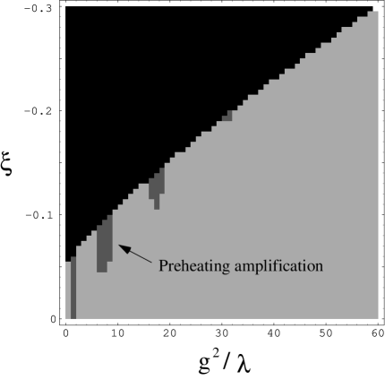
FIG. 3.: A density plot in the ($g^{2}/\lambda,\xi$)-plane where the super-Hubble curvature perturbations ${\cal R}$ is enhanced or not. The black color and the dark gray colours correspond to ranges where ${\cal R}$ grows during inflation, and during preheating, respectively. The region where ${\cal R}$ does not vary is shown by the light gray color. Note that there exist parameter ranges around the center of resonance bands ($g^{2}/\lambda=2n^{2}$) where ${\cal R}$ grows during preheating even for $g^{2}/\lambda\geq 8$. However, these regions do not persist for $g^{2}/\lambda>40$ as explained in the text.

In the case of the massive inflaton and a $g^{2}\phi^{2}\chi^{2}$ coupling, the effective mass of $\chi$ is approximately given by $m_{\rm eff}^{2}\approx[g^{2}+16\pi\xi(m/M_{pl})^{2}]\phi^{2}$ during inflation. This implies that it is not possible to achieve both the requirement of a light $\chi$ mass during inflation and a large $\chi$ mass ($q\gg 1$) after inflation and hence ${\cal R}$ is not enhanced during preheating even in the presence of nonminimal coupling.

This situation changes, however, if we consider a cubic coupling of the form $\tilde{g}^{2}\phi\chi^{2}$ instead. This still leads to preheating but now we can make $m_{\rm eff}^{2}$ light during inflation in certain regions of the $(\tilde{g}/m,\xi)$ parameter space, analagous to those in Fig. 3.

B Hybrid and Double inflation

In hybrid and supernatural inflationary models [29, 30, 31], a symmetry breaking transition occurs in the presence of a second scalar field, $N$. This leads to a negative coupling/tachyonic instability in which the longest wavelengths grow the strongest. Hence, even in the case when the spectrum of $N$ fluctuations is blue, this long-wavelength instability may lead to variation of ${\cal R}$ in certain cases.

To investigate this in detail, consider Linde’s hybrid inflation potential [29] with two scalar fields $\phi$ and $N$:

$$V=\frac{\lambda}{4}\left(N^{2}-\frac{M^{2}}{\lambda}\right)^{2}+\frac{1}{2}g^{2}N^{2}\phi^{2}+\frac{1}{2}m^{2}\phi^{2}\,.$$ (16)

Note that the supersymmetric version of the hybrid inflation corresponds to the case, $g^{2}/\lambda=2$ [30]. Hereafter we shall analyze the case where $g^{2}$ and $\lambda$ are the same order.

Inflation takes place due to the slow-roll evolution of $\phi$ before the field reaches a bifurcation point $\phi_{c}=M/g$. If the condition $m^{2}\phi_{c}^{2}\ll M^{4}/\lambda$ is satisfied, the Hubble constant at $\phi=\phi_{c}$ is given by $H=H_{0}\equiv\sqrt{2\pi/(3\lambda)}M^{2}/M_{\rm pl}$. It is convenient to normalize the masses of two fields $\phi$ and $N$ relative to $H_{0}^{2}$ as

$$\alpha\equiv\frac{m^{2}}{H_{0}^{2}}=\frac{3\lambda m^{2}M_{\rm pl}^{2}}{2\pi M^{4}},~{}~{}~{}~{}\beta\equiv\frac{M^{2}}{H_{0}^{2}}=\frac{3\lambda M_{\rm pl}^{2}}{2\pi M^{2}}\,.$$ (17)

$\alpha$ is required to be smaller than unity in order to lead to sufficient inflation for $\phi>\phi_{c}$. The evolution of the fluctuation $\delta N$ depends on the value of $\beta$ as we will classify below.

1 Light $N$ field (Double inflation)

When the $N$ mass is light ($\beta~{}\mbox{\raisebox{-4.30554pt}{$\stackrel{{\scriptstyle\textstyle<}}{{\textstyle\sim}}$}}~{}1$), the field $N$ and its large scale perturbation are free from inflationary suppression ($\phi>\phi_{c}$). In this case the coupling $\lambda$ is constrained to be small, $\lambda~{}\mbox{\raisebox{-4.30554pt}{$\stackrel{{\scriptstyle\textstyle<}}{{\textstyle\sim}}$}}~{}(M/M_{\rm pl})^{2}$. In order to end inflation due to a rapid rolling of the field $N$ after the symmetry breaking, one requires the “water-fall” condition $M^{3}\ll\lambda mM_{\rm pl}^{2}$ [29]. If we adopt the COBE normalization, $gM^{5}/(\lambda^{3/2}m^{2}M_{\rm pl}^{3})\simeq 3.5\times 10^{-5}$, which comes from the single-field fluctuation $\delta\phi$, the water-fall condition is not typically satisfied due to small $\lambda$. In this case the second stage of inflation occurs after the symmetry breaking (double inflation).

FIG. 4.: The evolution of super-Hubble cosmological perturbations in the case of a light $N$ mass with potential (16) as a function of $\tilde{t}\equiv\sqrt{2}Mt$ using the Hartree approximation. We choose the initial conditions to be $\phi=1.5\phi_{c}$ and $N=10^{-3}M/\sqrt{\lambda}$. We also show the evolution of adiabatic and entropy field perturbations, denoted by $\delta\sigma$ and $\delta s$, respectively.

Let us present a concrete example. In Fig. 4 we plot the evolution of ${\cal R}$ and $\Phi$ for $M=5.0\times 10^{-6}M_{\rm pl}$, $g^{2}=\lambda=8.0\times 10^{-11}$, and $m=0.2M$, corresponding to mass parameters $\alpha=0.07$ and $\beta=1.5$. In this case the first stage of inflation ($\phi>\phi_{c}$) continues around $\tilde{t}\equiv\sqrt{2}Mt\simeq 33$, after which the second phase of inflation takes place until $\tilde{t}\simeq 130$. The total number of e-folds is $N\sim 70$ for the initial value, $\phi=1.5\phi_{c}$.

In Fig. 4 we find that the entropy perturbation $\delta s$ is not strongly suppressed and begins to increase after the symmetry breaking due to tachyonic growth of the fluctuation $\delta N$. This can lead to the amplification of super-Hubble curvature perturbations until the backreaction of field fluctuations shuts off its growth.

Note that we implement the field backreaction effect at second order in our simulations. Since the fluctuation $\delta N$ is efficiently amplified in the tachyonic instability region, its growth terminates before the field $N$ reaches the potential minimum. The excitation of entropy perturbations also leads to the amplification of adiabatic field perturbations $\delta\sigma$ since they are correlated each other. In Fig. 4 we clearly find that the gravitational potential exhibits nonadiabatic growth sourced by the growth of $\delta\sigma$.

During reheating no enhancement of super-Hubble cosmological perturbations occurs in this case, since field perturbations are already excited until the beginning of the oscillating phase. This illustrates the importance of the spinodal instability region, during which ${\cal R}$ and $\Phi$ are amplified as well as field perturbations.

2 Heavy $N$ field (Hybrid inflation)

When $\beta\gg 1$, the field $N$ is exponentially suppressed during inflation ($\phi>\phi_{c}$). In this case the water-fall condition is typically satisfied after symmetry breaking, which corresponds to the original hybrid inflationary scenario [29] where inflation ends due to the rapid rolling of the field $N$.

The evolution of fluctuations for $\phi<\phi_{c}$ can be described similarly as the models of spontaneous symmetry breaking analyzed in Ref. [32]. The field $N$ has practically no homogeneous component at $\phi=\phi_{c}$. In this case the decomposition of $N$ between the homogenous field $N(t)$ and the fluctuational part $\delta N({\bf x},t)$ is not necessarily valid. Rather one is required to go beyond perturbation theory by considering the full spatial distribution of the field $N({\bf x},t)$.

FIG. 5.: The evolution of the large scale curvature perturbation in the heavy $N$ case with $M=3.0\times 10^{-6}M_{\rm pl}$, $g^{2}=\lambda=1.0\times 10^{-8}$ using the Hartree approximation to evaluate the backreaction. The result (i) is obtained by integrating Eq. (3), which is different from the result (ii) obtained by the definition ${\cal R}=\Phi-H/\dot{H}(\dot{\Phi}+H\Phi)$. In the case (ii) the field $\sigma$ is strongly dumped in Eq. (11) due to overestimation of the field variance, thereby leading to the decrease of $\Phi$ and ${\cal R}$. In the case (i) the damping of $\sigma$ provides a source term for $\dot{\cal R}$.

If the perturbative approach based on the Hartree approximation is applied, the effective mass of the field $N$ around $\phi=0$ is approximately given by $m_{N}^{2}\simeq 3\lambda\langle\delta N^{2}\rangle-M^{2}$. Naively one may expect that symmetry can be restored due to the growth of $\delta N$ with $\langle\delta N^{2}\rangle\simeq M^{2}/\lambda$, i.e., $m_{N}^{2}\simeq 2M^{2}$. Numerically we have found that the Hartree approximation leads to symmetry restoration. However we have to caution that this approach neglects the rescattering effect and the formation of topological defects. The authors in Ref. [32] found that the field distribution reaches the potential minimum at $N=M/\sqrt{\lambda}$ and $\phi=0$ instead of restoring symmetry when using the 3-D lattice simulations without metric perturbations. It was also pointed out that tachyonic growth of the field fluctuation is typically followed by only a single oscillation of the field.

In the Hartree approximation, the backreaction due to the growth of long wavelength fluctuations prevents the field from reaching the potential minimum due to an overestimation of the field variance. In Fig. 5 we find that the evolution of ${\cal R}$ differs significantly when we integrate Eq. (3) or evaluate ${\cal R}$ in terms of $\Phi$. This disagreement obviously shows the limitations of linearized gravity using the Hartree approximation. It is certainly of interest to analyze the evolution of super-Hubble cosmological perturbations in the heavy $N$ case including full nonlinear effects along the lines in Ref. [33, 34].

V Conclusion and Discussion

We discussed general principles governing the conditions under which the large scale curvature perturbation, ${\cal R}$ - used to normalize models to the large angle CMB anisotropies - is amplified after (and during) inflation.

This is closely allied with the evolution of entropy/isocurvature field perturbations $\delta s$ during the inflationary phase. If the mass of $\delta s$ is light relative to the Hubble rate, it sources the variation of the curvature perturbation when it is amplified during preheating or in the tachyonic instability region.

In the model with $V=\frac{1}{2}m^{2}\phi^{2}+\frac{1}{2}g^{2}\phi^{2}\chi^{2}$, super-Hubble entropy ($\delta s$) modes are exponentially suppressed during inflation for the coupling $g$ required to have efficient preheating. Therefore growth of $\delta s$ during preheating is not sufficient to lead to the variation of ${\cal R}$ on large scales. This situation is not altered in the model $V=\frac{1}{2}m^{2}\phi^{2}+\frac{1}{2}g^{2}\phi^{2}\chi^{2}+\tilde{g}^{2}\phi^{3}\chi$ where the fields evolve along the straight line ($\dot{\theta}\simeq 0$) during inflation [22].

In the model with $V=\frac{1}{4}\lambda\phi^{4}+\frac{1}{2}g^{2}\phi^{2}\chi^{2}+\frac{1}{2}\xi R\chi^{2}$, we found that parameter ranges where large scale curvature perturbations are amplified during preheating are significantly wider for negative nonminimal couplings.

We also studied hybrid/double inflationary models where tachyonic/spinodal instability of the symmetry breaking field $N$ leads to the growth of entropy field perturbations. When the field $N$ is light in the first stage of inflation, super-Hubble curvature perturbations typically exhibit tachyonic growth after the symmetry breaking. If the field $N$ is heavy, which is the original version of the hybrid inflationary scenario, we find that linearized gravity theory using the Hartree approximation shows some limitation in the sense that the evolution of ${\cal R}$ is different depending on which definition of ${\cal R}$ is used.

In the case of a purely quantum field with no classical vacuum expectation value (vev) - such as a fermion field or a scalar field whose vev vanishes during inflation such as discussed in Sec. IV B - a natural question arises: “what are the correct perturbed Einstein field equations?” It would be very useful to develop a formalism in which these quantum fields were treated non-perturbatively and self-consistently.

Finally, does inclusion of rescattering leads to extra variation of ${\cal R}$ or does causality protects ${\cal R}$ (and suitable nonlinear generalizations) to all orders in perturbation theory [35] in the absence of large-scale entropy perturbations? These interesting issues are left to future work.

ACKOWLEDGMENTS

We thank Robert H. Brandenberger for detailed and insightful comments on the draft and Takahiro Tanaka for useful discussions. ST is grateful for kind hospitality during his stay at the University of Portsmouth. BB receives support from EPSRC grant GR/R16488/01; ST thanks for financial support from the JSPS (No. 04942).

REFERENCES

- [1] A. D. Linde, Particle Physics and Inflationary Cosmology (Harwood, Chur, Switzerland, 1990); A. R. Liddle and D. H. Lyth, Cosmological inflation and Large-Scale Structure (Cambridge University Press, 2000).
- [2] A. H. Guth, Phys. Rev. D 23, 347 (1981); K. Sato, Mon. Not. R. Astron. Soc. 195, 467 (1981).
- [3] M. Gasperini and G. Veneziano, Astropart. Phys. 1, 317 (1993); J. Khoury, B. A. Ovrut, P. J. Steinhardt, and N. Turok, Phys. Rev. D 64, 123522 (2001); hep-th/0109050; P. J. Steinhardt, and N. Turok, hep-th/0111030; hep-th/0111098.
- [4] C. B. Netterfield et al., astro-ph/0104460 (2001).
- [5] J. Traschen and R. H. Brandenberger, Phys. Rev. D 42, 2491 (1990); Y. Shatanov, J. Trashen, and R. H. Brandenberger, Phys. Rev. D 51, 5438 (1995).
- [6] L. Kofman, A. D. Linde, and A. A. Starobinsky, Phys. Rev. Lett. 73, 3195 (1994); Phys. Rev. D 56, 3258 (1997).
- [7] D. Boyanovsky et al., Phys. Rev. D 51, 4419 (1995); D 56, 7570 (1996).
- [8] G. F. Giudice, A. Riotto, I. Tkachev, JHEP 0106 , 020 (2001); A. Maroto, hep-ph/0111126.
- [9] A. M. Green and K. A. Malik, Phys. Rev. D 64, 021301; B. A. Bassett and S. Tsujikawa, Phys. Rev. D 63, 123503 (2001).
- [10] A. Taruya and Y. Nambu, Phys. Lett. B428, 37 (1998).
- [11] B. A. Bassett, D. I. Kaiser, and R. Maartens, Phys. Lett. B455, 84 (1999).
- [12] F. Finelli and R. H. Brandenberger, Phys. Rev. Lett. 82, 1362 (1999).
- [13] B. A. Bassett, F. Tamburini, D. I. Kaiser, and R. Maartens, Nucl. Phys. B 561, 188 (1999).
- [14] K. Jedamzik and G. Sigl, Phys. Rev. D 61, 023519 (2000); P. Ivanov, Phys. Rev. D 61, 023505 (2000); S. Tsujikawa, JHEP 07, 024 (2000); A. R. Liddle, D. H. Lyth, K. Malik, and D. Wands, Phys. Rev. D 61, 103509 (2000).
- [15] B. A. Bassett, C. Gordon, R. Maartens, and D. I. Kaiser, Phys. Rev. D 61, 061302 (R) (2000).
- [16] B. A. Bassett and F. Viniegra, Phys. Rev. D 62, 043507 (2000).
- [17] A. B. Henriques and R. G. Moorhouse, Phys. Rev. D 62, 063512 (2000); Phys. Lett. B492, 331 (2000).
- [18] F. Finelli and R. H. Brandenberger, Phys. Rev. D 62, 083502 (2000).
- [19] S. Tsujikawa, B. A. Bassett, and F. Viniegra, JHEP 08, 019 (2000).
- [20] J. P. Zibin, R. H. Brandenberger, and D. Scott, Phys. Rev. D 63, 043511 (2001).
- [21] J. P. Zibin, hep-ph/0108008.
- [22] C. Gordon, D. Wands, B. A. Bassett, and R. Maartens, Phys. Rev. D 63, 023506 (2001).
- [23] D. S. Salopek, J. R. Bond, and J. M. Bardeen, Phys. Rev. D 40, 1753 (1989); D. Polarski and A. A. Starobinsky, Phys. Rev. D 50, 6123 (1994); A. A. Starobinsky and J. Yokoyama, gr-qc/9502002; J. García-Bellido and D. Wands, Phys. Rev. D 53, 437 (1995). M. Sasaki and E. D. Stewart, Prog. Theor. Phys. 95, 71 (1996).
- [24] S. Yu. Khlebnikov and I. I. Tkachev, Phys. Rev. Lett. 79, 1607 (1997).
- [25] P. B. Greene, L. Kofman, A. D. Linde, and A. A. Starobinsky, Phys. Rev. D 56, 6175 (1997); D. I. Kaiser, Phys. Rev. D 56, 706 (1997).
- [26] B. A. Bassett, M. Peloso, L. Sorbo, and S. Tsujikawa, Nucl. Phys. B 622, 393 (2002).
- [27] S. Tsujikawa and H. Yajima, Phys. Rev. D 62, 123512 (2000).
- [28] A. A. Starobinsky, S. Tsujikawa, and J. Yokoyama, Nucl. Phys. B610, 383 (2001).
- [29] A. D. Linde, Phys. Lett. B259, 38 (1991); Phys. Rev. D 49, 748 (1994).
- [30] E. J. Copeland, A. R. Liddle, D. H. Lyth, E. D. Stewart, and D. Wands, Phys. Rev. D 49, 6410 (1994).
- [31] L. Randall, M. Soljačić, and A. H. Guth, Nucl. Phys. B 472, 377 (1996); hep-ph/9601296.
- [32] G. Felder et al., Phys. Rev. Lett. 87, 011601 (2001); Phys. Rev. D 64, 123517 (2001).
- [33] M. Parry and R. Easther, Phys. Rev. D 59, 061301 (1999); D 62, 103503 (2000).
- [34] F. Finelli and S. Khlebnikov, Phys. Lett. B 504, 309 (2001).
- [35] T. Tanaka, Private Communication (2001).