Polarization of the Broad H$\alpha$ Wing in Symbiotic Stars

Abstract

In many symbiotic stars there appear broad wings around H$\alpha$, of which the formation mechanisms proposed thus far include a fast outflow, motion of the inner accretion disc, electron scattering and Raman scattering of Ly$\beta$. We adopt a Monte Carlo technique to simulate the Raman scattering of ultraviolet photons that are converted into optical photons around H$\alpha$, forming broad wings, and compute its polarization. Noting that many symbiotic stars exhibit a bipolar nebular morphology and polarization flip in the red-wing part of the Raman scattered O VI features, we assume that the neutral scattering region is composed of the two components. The first component is a static cylindrical shell with finite thickness; and the second component is a finite slab that is moving away with velocity $v_{p}=100{\rm\ km\ s^{-1}}$ along the symmetry axis of the first component. The cylindrical shell component yields polarization in the direction parallel to the cylinder axis. The strongest polarization is obtained in the limit where the height of the cylinder approaches zero and the scattering region effectively becomes a circular ring. As the height of the cylinder increases, the resultant polarization decreases and becomes negligible in the limit of the infinite cylinder. The polarization near the line-centre is weaker than in the far wing regions because of the large Rayleigh scattering numbers due to the large scattering cross sections near the line centre. The receding polar scattering component produces strong polarization in the direction perpendicular to the cylinder axis. In the presence of a Ly$\beta$ emission-line component with an equivalent width $\sim 0.5{\rm\ \AA}$, the polarized flux exhibits a local maxima at $\lambda=6578{\rm\ \AA}$ that corresponds to the receding velocity with $6.4v_{p}$ relative to H$\alpha$. When the both scattering components co-exist, the polarization is characterized by weak parallel polarization near the line-centre and strong perpendicular polarization in the red part. We discuss the observational implications of our computation.

1 Introduction

Symbiotic stars are generally known to be interacting binaries of a mass losing giant and a hot white dwarf surrounded by an ionized nebula which is responsible for various prominent emission lines (Kenyon, 1986). In the spectra of symbiotic stars, there exist very unique emission features around $6830{\rm\ \AA}$ and $7088{\rm\ \AA}$. Schmid (1989) proposed that they are formed via Raman scattering by atomic hydrogen of O VI 1032, 1038 doublet. When an O VI line photon that is more energetic than Ly$\alpha$ is incident upon a hydrogen atom in its ground $1s$ state, it subsequently re-emits an outgoing photon with de-excitation into either $1s$ state or $2s$ state. In the first case, we have a Rayleigh scattering process with no change in the frequency in the rest frame of the scatterer. The second case corresponds to a Raman scattering process, from which we obtain 6830 and 7088 line photons from incident O VI 1032 and 1038 photons, respectively.

The scattering cross-sections associated with these Raman processes are of order $\sigma\sim 10^{-23}{\rm\ cm^{2}}$ (e.g. Schmid, 1989; , 1989; Sadeghpour & Dalgarno, 1992; Lee & Lee, 1997), and therefore the operation of the O VI Raman scattering requires the existence of both a highly ionized O VI emission region and a fairly extensive neutral scattering region with H I column density $N_{HI}\sim 10^{23}\rm\ cm^{-2}$. The scattering cross section is very sensitive to the wavelength of the incident radiation in such a way that it steeply increases as the wavelength approaches the resonance wavelength of the scatterer. Therefore, continuum photons with wavelength near that of the Ly$\beta$ will be scattered in a neutral hydrogen region with much lower H I column density than that is required for O VI Raman scattering.

(1993) showed that most symbiotic stars in the southern hemishpere exhibit very broad wings around H$\alpha$. A similar result was reported for those in the northern hemisphere by Ivison, Bode & Meaburn (1994). The full width at zero intensity often exceeds $2000{\rm\ km\ s^{-1}}$. Similar broad wings also appear in young planetary nebulae, including M2-9, Mz3, and IC 4997 (e.g. , 1996; Arrieta & Torres-Peimbert, 2002). In particular, for M2-9, Balick (1989) reported the existence of very broad H$\alpha$ wings with a width $\sim 10^{4}{\rm\ km\ s^{-1}}$. Remarkably, Selvelli & Bonifacio (2000) presented the Very Large Telescope (VLT) spectrum of the symbiotic star RR Tel which shows H$\alpha$ wings extending up to $12000{\rm\ km\ s^{-1}}$. According to van de Steene, Wood & van Hoof (2000), post-asymptotic giant branch (post-AGB) stars also exhibit broad H$\alpha$ wings.

There have been many theoretical suggestions for formation mechanism of the broad H$\alpha$ wings. These include fast outflows (e.g. Schmutz et al., 1994), electron scattering (e.g. Bernat & Lambert, 1978), the accretion disc (e.g. Quiroga et al., 2002) and the Raman scattering of Ly$\beta$. In this paper, we will not consider all those theoretical models but will focus only on the H$\alpha$ wing formation via the Raman scattering of Ly$\beta$.

Nussbaumer et al. (1989) discussed the astrophysical importance of Raman scattering by atomic hydrogen and proposed that broad H$\alpha$ wings can be formed through the Raman scattering of Ly$\beta$. This idea has been applied to young and compact planetary nebula IC 4997 by Lee & Hyung (2000). They computed the wing profile formed through Raman scattering of flat continuum around Ly$\beta$ and obtained an excellent agreement with the observed profile. Similar success has been achieved for many symbiotic stars by Lee (2000).

The existence of a thick H I region in symbiotic stars and young planetary nebulae can also be inferred from the He II Raman scattered features. Because He II is also a single electron atom, the wavelengths associated with the transitions from $n=2m$ state to the $2s$ state are very close to those corresponding to the $m$th Lyman series of hydrogen. Therefore, He II Raman scattering requires much less H I column density $N_{HI}\sim 10^{20}{\rm\ cm^{-2}}$ than O VI 1032, 1038 doublet. The He II Raman-scattered lines have been found in the spectra of RR Tel and He 2-106 (e.g. van Groningen, 1993; Lee, Kang & Byun, 2001) and the young planetary nebulae M2-9 (Lee et al. 2001), which highlights the plausibility of the operation of the Ly$\beta$ Raman scattering in these objects. Therefore, in this work, we will consider Raman scattering of Ly$\beta$ in neutral regions with $N_{HI}=10^{20}-10^{23}\rm\ cm^{-2}$.

Spectropolarimetry will provide valuable information on the H$\alpha$ wing formation mechanism. Raman-scattered radiation consists of purely scattered radiation without any mixing of direct radiation, and therefore Raman-scattered radiation can be strongly polarized. Polarization is also dependent on the scattering geometry. Spectropolarimetry may reveal the circumstellar matter distribution and be useful to understand the mass-loss process of the giant component.

In this paper, we will compute the profile and the polarization of H$\alpha$ wings that are assumed to be formed through Raman scattering of Ly$\beta$. In section 2, we will briefly introduce the basic atomic physics relevant to the H$\alpha$ wing formation and describe the Monte Carlo procedure. In section 3, we present our main results. In the final section we discuss our results and observational implications.

2 H$\alpha$ Wing Formation through Raman Scattering

2.1 Branching Ratio

Figure 1: Branching ratio of the Raman scattering to the Rayleigh scattering. The solid and the long dashed lines represent the differential cross sections of Rayleigh and Raman scatterings in units of Thomson scattering cross section, respectively. The branching ratio of the Raman scattering to the Rayleigh scattering and its first-order approximation are shown in the dotted and the short dashed lines, respectively.

A Ly$\beta$ photon incident on a scattering region consisting of atomic hydrogen undergoes either Rayleigh scattering or Raman scattering. In particular, in the latter case the scattering H atom de-excites to the $2s$ state resulting in an outgoing H$\alpha$ photon. Owing to the scattering incoherency, if an incident photon near the Ly$\beta$ line centre is Raman-scattered, then the outgoing photon finds itself in the H$\alpha$ wing region much further from the line centre, by a factor of 6.4, than from the line centre of Ly$\beta$ (e.g. Schmid 1989, Nussbaumer et al. 1989). Lee & Hyung (2000) emphasized that the profile of H$\alpha$ wings formed by Raman scattering of Ly$\beta$ will be proportional to $\Delta\lambda^{-2}$, when the Raman scattering optical depth is small. However, the detailed conversion process from a ultraviolet photon into an optical photon is dependent on the branching ratio of the Rayleigh scattering and Raman scattering cross sections (e.g. Schmid 1996). In this subsection, we illustrate a basic calculation that provides an approximate branching ratio near the Ly$\beta$ line centre.

The branching ratio of the Rayleigh process to the Raman process is well known in the literature, which is around 1:7. However, this ratio is dependent on the wavelength of the incident photon.

The differential cross-section for Rayleigh scattering is given by

$${\left(d\sigma\over d\Omega\right)}_{\rm Ray}=r_{0}^{2}\left|{1\over m\hbar}\sum_{I}\left({\omega({\bf p}\cdot{\mbox{\boldmath$\epsilon$}}^{\alpha^{\prime}})_{AI}({\bf p}\cdot{\mbox{\boldmath$\epsilon$}}^{\alpha})_{IA}\over\omega_{IA}(\omega_{IA}-\omega)}-{\omega({\bf p}\cdot{\mbox{\boldmath$\epsilon$}}^{\alpha})_{AI}({\bf p}\cdot{\mbox{\boldmath$\epsilon$}}^{\alpha^{\prime}})_{IA}\over\omega_{IA}(\omega_{IA}+\omega)}\right)\right|^{2},$$ (1)

and the Raman scattering differential cross section is

$${\left(d\sigma\over d\Omega\right)}_{\rm Ram}=r_{0}^{2}\left({\omega^{\prime}\over\omega}\right)\left|{1\over m\hbar}\sum_{I}\left({({\bf p}\cdot{\mbox{\boldmath$\epsilon$}}^{\alpha^{\prime}})_{BI}({\bf p}\cdot{\mbox{\boldmath$\epsilon$}}^{\alpha})_{IA}\over\omega_{IA}-\omega}+{({\bf p}\cdot{\mbox{\boldmath$\epsilon$}}^{\alpha})_{BI}({\bf p}\cdot{\mbox{\boldmath$\epsilon$}}^{\alpha^{\prime}})_{IA}\over\omega_{IA}+\omega^{\prime}}\right)\right|^{2},$$ (2)

where the subscript $A$ stands for the initial quantum state of the scatterer, $I$ for the intermediate state and $B$ for the final state. We have $A=1s,B=2s$ for the Raman process and $A=B=1s$ for the Rayleigh process (Sakurai, 1967). Here, $\omega_{IA}=\hbar^{-1}(E_{I}-E_{A})$ is the angular frequency for the transition between the initial state $A$ and the intermediate state $I$, $r_{0}$ is the classical electron radius, and ${\textit{\boldmath$\epsilon$}}^{\alpha}$ represents the polarization vector of the incident photon. The primed quantities correspond to those associated with the outgoing photon. In particular, the energy conservation relation for the Raman scattering case gives

$$\omega^{\prime}=\omega-\omega_{\alpha},$$ (3)

where $\omega_{\alpha}$ represents the angular frequency of the Ly$\alpha$ transition. We are interested only in scatterings occurring in the wing regime far from the resonance and therefore omit the damping term in the denominator of each transition matrix element.

For an incident photon around Ly$\beta$, $\omega\simeq\omega_{\beta}$ and the cross sections for both scattering processes are predominantly contributed by the first term in the summation corresponding to $I=3p$ in equations (1) and  (2). Since the angular distribution of the scattered radiation is the same for both processes, we can write the branching ratio $r_{b}$ of the cross-sections for Rayleigh scattering and Raman scattering as

$$r_{b}(\omega)=\left({\omega^{\prime}\over\omega^{3}}\right)\left|{A_{1}/\Delta\omega-A_{2}\over A_{3}/\Delta\omega-A_{4}}\right|^{2}\simeq\left({\omega_{\beta}-\omega_{\alpha}\over\omega_{\beta}}\right)\left({A_{1}\over{\omega_{\beta}A_{3}}}\right)^{2}\left[1+\left({\omega_{\beta}\over\omega_{\beta}-\omega_{\alpha}}-3+{{2\omega_{\beta}A_{2}}\over A_{1}}-{{2\omega_{\beta}A_{4}}\over A_{3}}\right){\Delta\omega\over\omega_{\beta}}\right],$$ (4)

where we set $\omega=\omega_{\beta}+\Delta\omega$, $|\Delta\omega|\ll\omega_{\beta}$.

The matrix elements that appear in equation (4) are explicitly given by

$$A_{1} = <2s\parallel p\parallel 3p><3p\parallel p\parallel 1s>,$$

$$A_{2} = \sum_{I\neq 3p}{<2s\parallel p\parallel I><I\parallel p\parallel 1s>\over\omega_{I1}-\omega_{\beta}-\Delta\omega}+\sum_{I\neq 3p}{<2s\parallel p\parallel I><I\parallel p\parallel 1s>\over\omega_{I1}+(\omega_{\beta}-\omega_{\alpha}+\Delta\omega)},$$

$$A_{3} = {{|<3p\parallel p\parallel 1s>|^{2}}\over{\omega_{\beta}}},$$

$$A_{4} = \sum_{I\neq 3p}{|<I\parallel p\parallel 1s>|^{2}\over\omega_{I1}(\omega_{I1}-\omega_{\beta}-\Delta\omega)}-\sum_{I\neq 3p}{|<I\parallel p\parallel 1s>|^{2}\over\omega_{I1}(\omega_{I1}+\omega_{\beta}+\Delta\omega)}.$$ (5)

It is noted that the summation extends to the continuum states, where the sum over all continuum states should be written in an integral form.

The explicit representations of the matrix elements are found in the literature (e.g. Karzas & Latter, 1961; Saslow & Mills, 1969; Berestetskii, Lifshitz & Pitaevskii, 1971) and a straightforward numerical computation gives $A_{1}/(\omega_{\beta}A_{3})=0.9268$, $\omega_{\beta}A_{4}/A_{3}=17.91$, $\omega_{\beta}A_{2}/A_{1}=-30.37$. These results are directly substituted into equation (4) to yield

$$r_{b}(\omega)\simeq 0.1342-12.50\Delta\omega/\omega_{\beta}.$$ (6)

In Fig. 1 we present the branching ratio of the Raman scattering cross-section to the Rayleigh cross section. The short-dashed line represents the approximate result given in equation (6), whereas the dotted line stands for the result obtained by using the whole Kramers-Heisenberg relation. The approximate relation gives an error of less than 10 per cent in the range $\Delta V\leq 1000{\rm\ km\ s^{-1}}$. This implies that the contribution from other $np$ states is not negligible. From Fig. 1 we see that the branching ratio varies in a rather large range from 0.05 to 0.45 in the wavelength interval from 1015 Å to 1040 Å. Since the broad feature around 7088 Å which is Raman-scattered O VI 1038 is often found in the spectra of symbiotic stars, it is necessary to investigate the Raman conversion efficiency for a broad range of the branching ratios.

2.2 Scattering Geometry

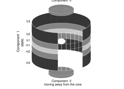
Figure 2: Schematic view of the scattering geometry. The central core represents the emission region. The static cylindrical shell denoted by Component I is composed of three layers stratified from the equatorial region. The layers are characterized by different H I densities and heights $h_{1},h_{2},h_{3}$. The circular slabs (Component II) with homogeneous H I density are located in the polar direction, moving away from the core.

Many symbiotic stars exhibit a bipolar nebular morphology, which is characterized by the accumulation of circumstellar materials near the equatorial plane. Many studies of Raman scattered O VI lines have demonstrated that the neutral scattering region can be associated with the cool component, while the ionized region must be close to the hot component (Harries & Howarth, 1997; Schmid & Schild, 1997; Schmid, Corradi, Krautter & Schild, 2000).

However, the Raman scattering of Ly$\beta$ becomes significant in neutral regions with $N_{HI}\geq 10^{20}\rm cm^{-2}$, which is two orders of magnitude smaller than the column density required for the operation of O VI Raman scattering. This implies that the H$\alpha$ wing formation through Ly$\beta$ Raman scattering should occur in much more extended regions than those that can be probed by Raman-scattered O VI features. This is consistent with the fact that most symbiotic stars exhibit broad H$\alpha$ wings whereas only about half of them show Raman-scattered O VI features (van Winckel et al. 1993, Ivison et al. 1994). Furthermore, broad H$\alpha$ wings are also found in young planetary nebulae and post-AGB stars, which appear to have common characteristics including bipolar morphology and composite emission-line profiles (Arrieta & Torres-Peimbert, 2002). It is still uncertain that all these objects are binary systems, whereas symbiotic stars are generally regarded as binary systems. In view of these circumstances, we adopt a simple neutral scattering region that is approximated by a cylindrical shell.

Fig. 2 shows a schematic view of the scattering geometry. We just assume that the neutral hydrogen component forms a finite cylindrical shell (Component I in Fig. 2) with the centre coinciding with the Ly$\beta$ emission source. The cylindrical shell is assumed to be of constant H I density and hence characterized by radius $r$ and height $h$.

In the spectropolarimetric data presented by Harries & Howarth (1996), the Raman-scattered O VI 6830 and 7088 features exhibit polarization flip in the red-wing part. Schmid (1996) interpreted the polarization flip in the red-wing part by scattering in the slow stellar wind from the giant component. Another interpretation has been proposed by Lee & Park (1999), who assumed the existence of an accretion disc around the white dwarf component via gravitational capture of the slow stellar wind around the giant component. According to their model, the emission region is formed around the accretion disc, and the main double peaks shown in the Raman-scattered features are attributed to the disc motion viewed in the equatorial direction, where the main scattering region is formed around the giant component. In order to explain the polarization flip in the red-wing part, there has to be another scattering component that is moving away from the emission region in the direction perpendicular to the equatorial plane.

In this work, we will also consider that H$\alpha$ wings are significantly contributed by this polar scattering region (Component II in Fig. 2). It is uncertain whether this polar scattering component is ubiquitous in all symbiotic stars. Harries & Howarth (1996) showed that a significant fraction of symbiotic stars may possess this component, in the picture presented by Lee & Park (1999). Because the polar component is assumed to be receding from the emission region, it will mainly affect the red part of the H$\alpha$ wings.

With this geometry, we prepare a photon source at the centre, from which the ultraviolet photons around Ly$\beta$ are injected into the scattering region. For a given incident photon the corresponding cross-sections of the Rayleigh and the Raman scatterings are calculated from the Kramers-Heisenberg formula (e.g., Bethe & Salpeter, 1957; Sakurai, 1967). The ratio of the two cross-sections is dependent only upon the incident wavelength (Lee & Lee, 1997). According to this ratio, we decide whether a given scattering event is Rayleigh or Raman in the Monte Carlo procedure.

Although the ultraviolet photons may be Rayleigh-scattered several times, the scattering regions are assumed to be transparent to the optical photons converted by Raman scattering. Therefore an incident ultraviolet photon suffers a number of Rayleigh scatterings until it is Raman scattered or escapes the scattering region as an ultraviolet photon.

We typically inject $10^{5}$ ultraviolet photons into a bin with $\Delta\lambda=0.005\rm\ \AA$ around Ly$\beta$, and calculate the polarization state at each scattering. Finally we collect Raman scattered photons according to the emergent direction cosine of the wave vector with a bin size of $\Delta\mu=0.1$.

2.3 Computation of Polarization

Because our scattering geometry is azimuthally symmetric, under the assumption that the emission source is not circularly polarized, no circular polarization will develop. Hence we only consider linear polarization that may develop either in parallel or perpendicular to the symmetry axis. We will distinguish the polarization direction by the sign of the polarization. That is, we will denote the polarization perpendicular to the symmetry axis by positive polarization and parallel polarization by negative polarization.

In the case of single electron atoms including hydrogen, the fine structure level splitting is small because of accidental degeneracy. Therefore any off-resonance scattering is characterized by the same scattering phase function as that of the Thomson scattering, which was shown by Stenflo (1980). Since the H$\alpha$ wings spread over $\geq 1000{\rm\ km\ s^{-1}}$, resonance scattering contributes very little to the wing formation. Hence, in this work, the relevant scattering phase function is that for Thomson scattering.

In the computation of linear polarization, we adopt the density matrix formalism, in which the polarization state is described by a $2\times 2$ Hermitian matrix $\rho$. In particular, with respect to the symmetry axis which is taken as the $z$-axis in the usual spherical coordinate, we choose the polarization basis vectors by ${\textit{\boldmath$\epsilon$}}_{1}=(\sin\phi,-\cos\phi,0)$, ${\textit{\boldmath$\epsilon$}}_{2}=(\cos\theta\cos\phi,\cos\theta\sin\phi,\sin\theta)$ for a given line photon with wavevector ${\hat{\textit{\boldmath$k$}}}=(\sin\theta\cos\phi,\sin\theta\sin\phi,\cos\theta)$, the linear polarization $p$ is obtained from the difference of the main diagonal elements of the density matrix $\rho$,

$$p=\rho_{11}-\rho_{22}.$$ (7)

The relation between the density matrix $\rho^{\prime}$ of the scattered radiation with wavevector ${\hat{\textit{\boldmath$k$}}^{\prime}}=(\sin\theta^{\prime}\cos\phi^{\prime},\sin\theta^{\prime}\sin\phi^{\prime},\cos\theta^{\prime})$ and $\rho$ of the incident radiation is given by

$$\rho_{11}^{\prime}=\rho_{11}\cos^{2}\Delta\phi-\rho_{12}\cos\theta\sin 2\Delta\phi+\rho_{22}\cos^{2}\theta\sin^{2}\Delta\phi,$$ (8)

$$\rho_{12}^{\prime}={1\over 2}\rho_{11}\cos\theta^{\prime}\sin 2\Delta\phi+\rho_{12}(\cos\theta\cos\theta^{\prime}\cos 2\Delta\phi+\sin\theta\sin\theta^{\prime}\cos\Delta\phi)-\rho_{22}\cos\theta(\sin\theta\sin\theta^{\prime}\sin\Delta\phi+{1\over 2}\cos\theta\cos\theta^{\prime}\sin 2\Delta\phi),$$

$$\rho_{22}^{\prime}=\rho_{11}\cos^{2}\theta^{\prime}\sin^{2}\Delta\phi+\rho_{12}\cos\theta^{\prime}(2\sin\theta\sin\theta^{\prime}\sin\Delta\phi+\cos\theta\cos\theta^{\prime}\sin 2\Delta\phi)+\rho_{22}(\cos\theta\cos\theta^{\prime}\cos\Delta\phi+\sin\theta\sin\theta^{\prime})^{2},$$

where $\Delta\phi=\phi^{\prime}-\phi$.

It can be also shown that the angular distribution of the scattered radiation for an incident photon with ${\hat{\textit{\boldmath$k$}}}$ and $\rho$ is given by the trace of $\rho^{\prime}(\theta^{\prime},\phi^{\prime},\theta,\phi)$ (e.g. Lee, Blandford & Western, 1994). Therefore, once the wavevector ${\hat{\textit{\boldmath$k$}}^{\prime}}$ of a scattered photon is chosen from $\rho^{\prime}$, the polarization is also determined at the same time. It is also noted that the density matrix is normalized each time so that it has a unit trace.

3 Results

First, we present two idealized cases in order to obtain a qualitative understanding of the polarization development through Raman scattering. Next, adopting a simple geometry we calculate the profile and the polarization for various geometrical parameters. Then we present two applications for more realistic geometries.

3.1 Infinite Slab

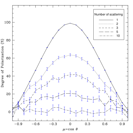
Figure 3: Polarization of the Raman scattered photons for various lines of sight. Ultraviolet photons are normally incident on an infinite slab with a finite thickness. Various types of lines represent the number of scatterings that outgoing photons suffer. The polarization is set to be positive when the polarization direction is perpendicular to the slab normal. The horizontal axis represents the cosine of the angle ($\mu=cos\theta$) between the slab normal and the line of sight. The error bars represent one standard deviation.

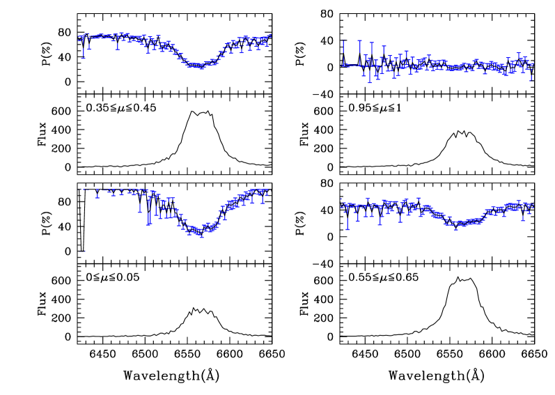
Figure 4: Profiles and polarization of Raman scattered photons for various lines of sight. $10^{4}$ ultraviolet photons are injected normally on to the infinite slab. The H I column density is set to be $5\times 10^{20}\rm cm^{-2}$. The error bars represent one standard deviation.

To investigate the dependence of the polarization on the number of Rayleigh scattering that a photon suffers, we just focus on the scattering events, ignoring other effects. An incident photon can escape and be counted only if it attains the prescribed number of scattering.

We typically prepare $10^{4}$ photons which are normally incident on an slab with a finite thickness. Here, we assume that the horizontal physical dimensions of the slab are infinite. We collect only those photons that have been scattered the prescribed number of times. We present the result in Fig. 3, where the horizontal axis represents the cosine of angle ($\mu=cos\theta$) between the slab normal and the line of sight. The polarization steeply decreases as the scattering number increases. If a photon is scattered three times, its maximal polarization reduces to about 40 per cent, and almost zero polarization is observed when the number of scatterings exceeds 10. The general behaviour of polarization weakening as a result of increased number of scatterings can be found in the literature (e.g. Angel, 1969).

Next, we present an idealized case of incidence normal to the slab in Fig. 4. We also inject $10^{4}$ ultraviolet photons in a bin with $\Delta\lambda=0.05\rm\ \AA$ with full width $6\rm\ \AA$ centred at Ly$\beta$. They are normally incident to the infinite slab lying in the $x-y$ plane. The H I column density is set to be $5\times 10^{20}\rm cm^{-2}$.

Despite the large column density, for an incident ultraviolet photon far from the resonance wavelength of Ly$\beta$, the scattering region is optically thin and hence the Raman conversion rate is very low. However, radiation in this wing region is highly polarized up to 100 per cent in the equatorial direction, because the scattering number rarely exceeds 2.

As the wavelength goes close to the Ly$\beta$ line centre, the cross-section increases steeply. In this case, most incident ultraviolet photons may suffer a number of Rayleigh scatterings before escape by Raman scattering. They escape from the slab by the final Raman scattering and contribute to the broad H$\alpha$ wing formation. The flux near the Ly$\beta$ line centre is typically polarized by about 40 per cent in the equatorial direction, which is weaker than in the far-wing regions. The weakening of polarization in this region is attributed to the increased Rayleigh scattering numbers before escape.

3.2 Polarization for Various Heights of the Cylindrical Scattering Regions

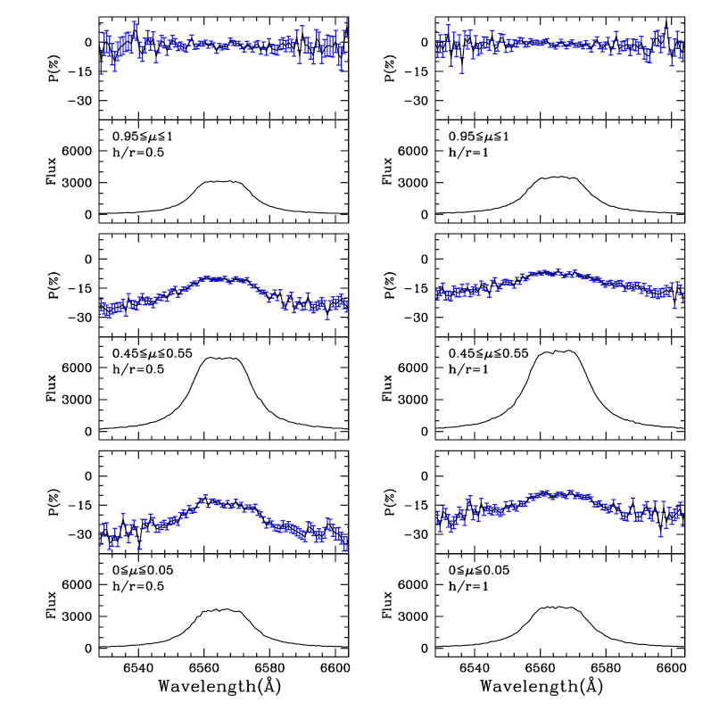
Figure 5: Profiles and polarization of broad H$\alpha$ wings for various lines of sight. Here we consider only Component I in Fig. 2 with $h\equiv h_{1}=h_{2}=h_{3}$. The height-to-radius ratios $h/r$ of the H I cylindrical shell are 0.5 and 1 for left- and right-hand panels, respectively. $10^{5}$ ultraviolet photons in a bin with $\Delta\lambda=0.005\rm\ \AA$ are injected to the H I component I. The homogeneous H I column density is set to be $10^{20}\rm cm^{-2}$. The error bars represent one standard deviation.

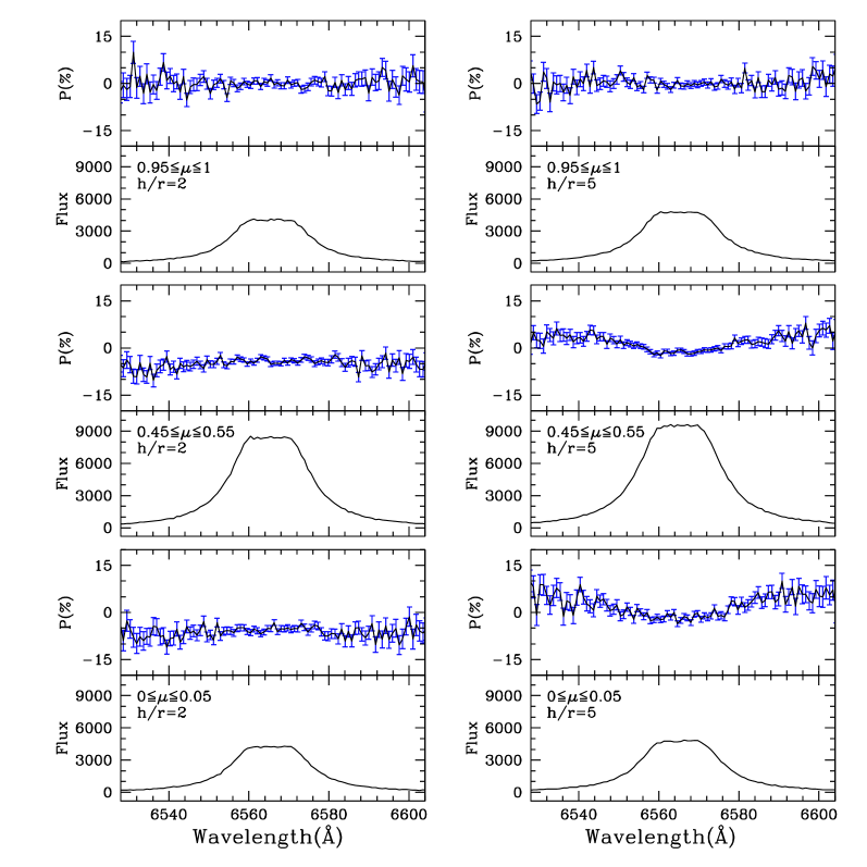
Figure 6: Profiles and polarization of broad H$\alpha$ wings for various lines of sight. The height-to-radius ratios of the H I cylinder are 2 and 5 for left- and right-hand panels, respectively. Other parameters are the same as described in Fig. 5

We assume that the H I number density is constant throughout the scattering region of Component I in Fig. 2 ($h\equiv h_{1}=h_{2}=h_{3}$), and obtain the profile and polarization of broad H$\alpha$ wings, changing the ratios $h/r$ of height to radius. In this work, just for simplicity and with a lack of detailed information on the circumstellar matter distribution, we assume that the thickness of the H I cylindrical shell is much smaller than the radius. The profiles and polarization of the broad H$\alpha$ wings for various lines of sight are shown for several ratios in Figs. 5 and  6.

The radiation emergent in the polar direction is almost unpolarized because of the symmetry, which provides a check of our code. When the observer is in the equatorial direction, the Raman scattered radiation exhibits negative polarization. As the height-to-radius ratio approaches zero, the scattering region is regarded as a circular ring, which yields the strongest polarization, 33 per cent, in the direction parallel to the symmetry axis of the circular ring. Since photons falling on to far-wing regions are scattered fewer times than those contributing to near-wing regions, the polarization in far-wing regions is much stronger than that near the H$\alpha$ centre. Therefore it is particularly notable that the Raman scattering wings are characterized by weak polarization near the centre and strong polarization at far-wing regions, in the direction of the symmetry axis.

As the height increases relative to the radius, for a given line of sight, there can be a broad range of scattering angles. Therefore a superposition of electric vectors associated with the scattered radiation lessens the overall polarization. In Fig. 6, it is apparent that the polarization weakens as $h/r$ increases. When $h/r=2$, we obtain H$\alpha$ wings polarized up to 10 per cent observed from the equatorial direction, which is much smaller than 30 per cent obtained in the case of $h/r=0.5$.

This trend will continue until the geometry is approximately regarded as an infinite cylinder. In this case, when the cylinder has enough thickness, emergent Raman-scattered wings will be contributed to equally from all directions of incidence, and will be completely unpolarized. We increase the ratio $h/r$ to as high as 5, which corresponds to the case that ultraviolet radiation from the emission source with $\theta>10^{\circ}$ will be incident on to the scattering region. As is shown in upper panels of Figs. 5 and 6, we obtain negligible polarization in this case for all lines of sight.

However, we also see the weakly polarized parts in far blue and red regions for the case $h/r=5$. This polarization, developed in the direction perpendicular to the symmetry axis, is attributed to the limb effect. That is, the cylindrical shell is optically thin in the direction normal to the shell for far blue- or red-wing photons. Therefore, only a small fraction $\tau_{w}$ of photons incident in this direction will be scattered, where $\tau_{w}$ is the Raman scattering optical depth in this direction. However, when the incident photon has the wavevector ${\hat{\textit{\boldmath$k$}}}$ with ${\hat{\textit{\boldmath$k$}}}\cdot{\hat{\textit{\boldmath$z$}}}=\mu\simeq 1$, the fraction of scattered photons increases to ${\tau_{w}}/{\sqrt{1-\mu^{2}}}$ which is much larger than $\tau_{w}$. This limb effect strengthens the positive polarization component and results in polarization in the perpendicular to the symmetry axis.

In the cylinder scattering model, we may summarize by saying that the polarization develops in the direction parallel to the symmetry axis, and that the polarization is weaker near the H$\alpha$ centre, because of large number of the Rayleigh scatterings, than it is in the far-wing regions.

3.3 Hybrid Model of Cylindrical Shells

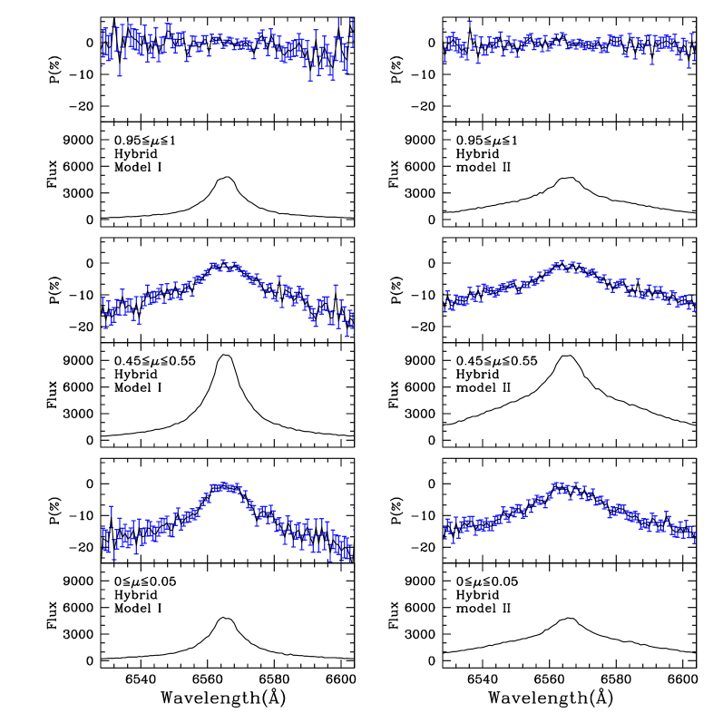
Figure 7: Profiles and polarization of broad H$\alpha$ wings for the hybrid model. We consider only Component I in Fig. 2. The H I column densities are set to be $10^{21},10^{20}$ and $10^{19}\rm\ cm^{-2}$ from the equatorial region with $h_{1},h_{2},h_{3}$=0.1, 0.5 and 5 in units of the radius $r$ for the Hybrid Model I, and 0.5, 1 and 5 for the Hybrid Model II. Other parameters are the same as described in Fig. 5.

We present a hybrid model of Component I in Fig 2 consisting of three stratified layers ($h_{1}<h_{2}<h_{3}$) with different H I column densities. In this model, the density is highest in the equatorial region and decreases as the latitude increases. This may mimic the matter distribution in the circumstellar region more realistically. This hybrid model can be viewed as a linear superposition which is the solid-angle-weighted sum of the previous models with various ratios and homogeneous hydrogen number density.

We consider two different cases denoted by Model I and Model II. In Model I, we set $h_{1}=0.1r$, $h_{2}=0.5r$ and $h_{3}=5r$; in Model II, we set $h_{1}=0.5r,\ h_{2}=r$ and $h_{3}=5r$. In both cases, the H I column densities of the stratified layers are chosen to be $N_{HI}=10^{21},\ 10^{20}$ and $10^{19}{\rm\ cm^{-2}}$, respectively.

We obtain similar patterns in polarization, which is weak near the H$\alpha$ centre and becomes strong in far-wing regions. These polarization patterns are also attributed to larger scattering numbers for photons near the line centre than those for far-wing photons.

It is particularly notable that a flat profile near the line centre no longer appears. This is because of the contribution made by the small column density regions at high latitudes. These regions are optically thin for most of incident ultraviolet photons, and hence yields profiles proportional to the scattering cross-section which is very steep near the line centre. In Model II shown in the right-hand panel of Fig. 7, the profile is fairly extensive because of the much larger column density than in the case of Model I shown in the left-hand panel of the same figure.

3.4 Raman Scattering from the Receding Polar Components

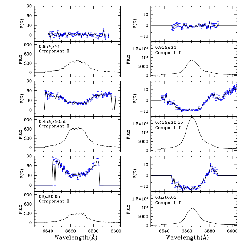
Figure 8: Profiles and polarization of broad H$\alpha$ wings for both components. We set the recession velocity of the scattering region of Component II to be $v_{p}=100\rm\ km\ s^{-1}$, the half-opening angle to be 20°  and the ratio of Component I ($h\equiv h_{1}=h_{2}=h_{3}$) to be $h/r=0.5$. $10^{5}$ ultraviolet photons in a bin with $\Delta\lambda=0.005\rm\ \AA$ are injected into only Component II with H I column density $10^{20}\rm\ cm^{-2}$ in the left-hand panel, and into both components (H I column density $10^{20}$, $10^{23}\rm\ cm^{-2}$ for Component I and Component II, respectively) in the right-hand panel. We omit to denote the polarization when the photon flux is negligibly small. The error bars represent one standard deviation.

In this subsection, we consider the Raman scattering from the receding polar scattering region of Component II, the existence of which is implied by Harries & Howarth (1996). In this work, we simply assume that this component is moving away from the emission source along the symmetry axis of the cylindrical shells considered in the previous subsections.

In the left-hand panel of Fig. 8 we show the polarization of H$\alpha$ wing photons Raman-scattered in the receding polar region. We set the recession velocity of the polar component to be $v_{p}=100{\rm\ km\ s^{-1}}$. Since the symmetry axis and the scattering plane make a very small angle, the polarization develops in the direction perpendicular to the symmetry axis, or in our formalism we obtain positive polarization. For an observer in the equatorial direction, the scattering angle is nearly 90^∘, and therefore almost complete polarization is obtained.

The wing flux is proportional to the scattering cross-section and the incident UV flux in the optically thin limit. In the observer’s rest frame, the scattering cross-section peaks at the recessional velocity of the polar component $v_{p}$, and therefore we obtain a small peak at this velocity. Hence the resultant profile is obtained effectively by shifting the wing flux that is formed from Raman scattering in a static medium. Owing to the incoherency of Raman scattering, the wing flux peaks at 6578 Å. This is interesting in that the symbiotic stars RR Tel and He 2-106 appear to exhibit a small and broad bump around 6580 Å just blueward of [N II] 6584 feature (Lee, Kang & Byun, 2001).

In the right-hand panel of Fig. 8, we present the Raman scattered wing fluxes obtained from combinations of a static cylindrical shell and a receding polar component. Since the two scattering components provide opposite senses of polarization, the resultant polarization is obtained by the algebraic sum of the two polarized flux components divided by the total flux. Therefore, in the blue wing, where the polar component contributes little, we obtain polarization in the direction parallel to the symmetry axis. However, in the red wing, the polar component predominantly contributes to the final polarization, yielding perpendicular polarization.

4 Discussion and Summary

We have investigated the polarization of H$\alpha$ wings formed through Raman scattering of Ly$\beta$. Two kinds of scattering regions are considered. The first one is a static cylindrical shell. From this component, the polarization of H$\alpha$ wings develops in the direction parallel to the cylinder axis. It is particularly notable that stronger polarization is obtained in far-wing regions than near the line centre. Near the line centre, the scattering cross-section is larger, and therefore Rayleigh scattering occurs more frequently than in the far-wing regions. The weaker polarization in the near-wing regions is attributed to the larger Rayleigh scattering numbers than in the far-wing regions.

We consider the second scattering component which is located in the polar regions and moving away from the ultraviolet emission source with a recessional velocity $v_{p}=100{\rm\ km\ s^{-1}}$. The physical nature of this component is not certain, but the existence of this component is apparent from the spectropolarimetric observations presented by Harries & Howarth (1996). This component produces polarization in the direction perpendicular to the symmetry axis. Since the scattering angle is almost $90^{\circ}$, nearly complete polarization is obtained. Since the scattering component is moving away from the source, the wing flux peak appears at $v=6.4v_{p}$, or around 6578 Å with our choice of $v_{p}=100{\rm\ km\ s^{-1}}$. Therefore, this polar component will produce a small bump in the wing profile which is strongly polarized in the direction perpendicular to the symmetry axis.

When the both scattering components co-exist, we may observe the polarization flip, where the blue part is characterized by parallel polarization and the red part is polarized in the perpendicular direction. Therefore, if the scattering region is composed of a cylindrical shell subtending a fairly large solid angle with sufficient column density and a small receding polar component, the overall wing profile is determined by the cylinder component and the polarization will be predominantly contributed by the polar component in the red part. Therefore in this case, we mainly obtain a profile that is nearly proportional to $\Delta\lambda^{-2}$ and strongly polarized in the red part in the direction perpendicular to the symmetry axis.

This is very interesting, considering the spectropolarimetric observation of the symbiotic star BI Crucis by Harries (1996), who reported the polarized H$\alpha$ wings in the direction perpendicular to the symmetry axis. They also noted that the polarization is very strong in the red part. In their spectropolarimetric data, no polarization flip is apparent. They interpreted their data using the assumption that the wings are formed through electron scattering. However, their data appear to be qualitatively consistent with the hypothesis that the H$\alpha$ wings are formed by Raman scattering in a fairly extensive cylindrical shell and a receding polar component.

Lee (1999) proposed that electron scattering of monochromatic line radiation may leave polarization structures. The radiative transfer process through Thomson scattering is diffusive both in real space and frequency space. This implies that photons that suffer more electron scattering tend to fall in both far- and near-wing regions, whereas those with fewer numbers of scatterings contribute to the formation of near-wing regions. Since polarization becomes weaker as the scattering number increases, we obtain weaker polarization in the far-wing regions in Thomson scattering media. Therefore spectropolarimetry can be an important tool to investigate the wing formation mechanism.

The Ly$\beta$ photon source was considered to be point-like. In reality, this photon source will be extended and even partly coincide with the scattering region. This will most likely lower the resulting polarization. The H$\alpha$ line flux will be strongly diluted by photons from the emission nebula, originating predominantly from the recombination process. This contribution can be dominant in the line centre and it will lower the resulting polarization considerably. Other factors that may affect the polarization of Raman-scattered H$\alpha$ wings and have not been considered in this work may include dust and the kinematics of the cylindrical shell component. Currently, only a few spectropolarimetric observations of H$\alpha$ wings can be found in the literature, and little is known about the formation of H$\alpha$ profiles seen in symbiotic stars. We hope that more observations will provide constraints on various theoretical models of H$\alpha$ and other Balmer series line formation.

References

- Angel (1969) Angel J. R. P., 1969, ApJ, 158, 219
- Arrieta & Torres-Peimbert (2002) Arrieta A., Torres-Peimbert S., 2002, Rev. Mex. Astron. Astrophys. 12, 154
- Balick (1989) Balick B., 1989, AJ, 97, 476
- Berestetskii, Lifshitz & Pitaevskii (1971) Berestetskii V. B., Lifshitz E. M., Pitaevskii V. B., 1971, Relativistic Quantum Theory, Pergamon Press, Oxford
- Bernat & Lambert (1978) Bernat A. P., Lambert D. L., 1978, PASP, 90, 520
- Bethe & Salpeter (1957) Bethe H. A., Salpeter E. E., 1957, Quantum Mechanics of One and Two Electron Atoms. Academic Press, New York
- Harries (1996) Harries T. J., 1996, A&A, 315, 499
- Harries & Howarth (1996) Harries T. J., Howarth I. D., 1996, A&AS, 119, 61
- Harries & Howarth (1997) Harries T. J., Howarth I. D., 1997, A&AS, 121, 15
- Ivison, Bode & Meaburn (1994) Ivison R. J., Bode M. F., Meaburn J., 1994, A&AS, 103, 201
- Karzas & Latter (1961) Karzas W. J., Latter R., 1961, ApJS, 6, 167
- Kenyon (1986) Kenyon S. J., 1986, The Symbiotic Stars. Cambridge Univ. Press, Cambridge
- Lee (1999) Lee H.-W., 1999, ApJ, 511, L13
- Lee (2000) Lee H.-W., 2000, ApJ, 541, L25
- Lee, Blandford & Western (1994) Lee H.-W., Blandford R. D., Western L., 1994, MNRAS, 267, 303
- Lee & Hyung (2000) Lee H.-W., Hyung S., 2000, ApJ, 530, L49
- Lee, Kang & Byun (2001) Lee H.-W., Kang Y. W., Byun Y.-I., 2001, ApJ, 551, L121
- Lee & Lee (1997) Lee H.-W., Lee K. W., 1997, MNRAS, 287, 211
- Lee & Park (1999) Lee H.-W., Park M.-G., 1999, ApJ, 515, 89
- (20) Miranda L. F., Torrelles J. M., Eiroa C., 1996, ApJ, 461, L111
- (21) Nussbaumer H., Schmid H. M., Vogel M., 1989, A&A, 211, L27
- Quiroga et al. (2002) Quiroga C., Mikolajewska J. Brandi E., Ferrer O., Garcia L., 2002, A&A, 387, 139
- Sadeghpour & Dalgarno (1992) Sadeghpour H. R., Dalgarno A., 1992, J. Phys. B: At. Mol. Opt. Phys., 25, 4801
- Sakurai (1967) Sakurai J. J., 1967, Advanced Quantum Mechanics., Addison-Wesley Publishing Company, Reading, MA.
- Saslow & Mills (1969) Saslow W. M., Mills D. L., 1969, Phys. Rev., 187, 1025
- Schmid (1989) Schmid H. M., 1989, A&A, 211, L31
- Schmid (1996) Schmid H. M., 1996, MNRAS, 282, 511
- Schmid, Corradi, Krautter & Schild (2000) Schmid H. M., Corradi R., Krautter J., Schild H., 2000, A&A, 355, 26
- Schmid & Schild (1997) Schild H., Schmid H. M., 1997, A&A, 324, 60
- Schmutz et al. (1994) Schmutz W., Schild H., Mürset U., Schmid H. M., 1994, A&A, 288, 819
- Selvelli & Bonifacio (2000) Selvelli P. L., Bonifacio P., 2000, A&A, 364, L1
- Stenflo (1980) Stenflo J. O., 1980, A&A, 84, 68
- van de Steene, Wood & van Hoof (2000) van de Steene G. C., Wood P. R., van Hoof P. A. M., 2000, in ASP Conf. Ser. 199, Asymmetrical Planetary Nebulae II: From Origins to Microstructures, ed. J. H. Kastner, N. Soker, & S. Rappaport (San Francisco: ASP), 191
- van Groningen (1993) van Groningen E., 1993, MNRAS, 264, 975
- (35) van Winckel H., Duerbeck H. W., Schwarz H. E., 1993, A&AS, 102, 401