Time-series Spectroscopy of Pulsating sdB Stars II: Velocity Analysis of PG1605+072

Abstract

We present the analysis of time-resolved spectroscopy of the pulsating sdB star PG 1605+072. From our main observing run of 16 nights we have detected velocity variations at 5 frequencies that correspond to those found in photometry. Based on these data, there appears to be change in amplitude of the dominant modes over about a year. However, when we include extra observations to improve the frequency resolution, we find that some of the frequencies are split into two or three. Simulations suggest that the apparent amplitude variation can be at least partially explained by a series of very closely spaced frequencies around the two strongest modes. By combining observations taken over $\sim$300 days we conclude that some of the closely spaced modes are caused by one mode whose amplitude is varying, however this frequency is still within $\sim$1 $\mu$Hz of an apparently stable frequency. Because of this kind of complexity and uncertainty we advise caution when trying to identify oscillation modes in this star.

1 Introduction

The discovery of pulsations in hot subdwarf B (sdB) stars provides an excellent opportunity to probe sdB interiors using asteroseismological analysis. While it is generally accepted that sdBs are the field analogues of Extreme Horizontal Branch (EHB) stars, many questions remain about their formation and evolution. Subdwarf B stars (like their EHB counterparts) are He-core burning, with 20 000 K $\mathrel{\mathchoice{\vbox{\offinterlineskip\halign{\hfil$\reset@font\displaystyle#$\hfil\cr<\cr\sim\cr}}}{\vbox{\offinterlineskip\halign{\hfil$\reset@font\textstyle#$\hfil\cr<\cr\sim\cr}}}{\vbox{\offinterlineskip\halign{\hfil$\reset@font\scriptstyle#$\hfil\cr<\cr\sim\cr}}}{\vbox{\offinterlineskip\halign{\hfil$\reset@font\scriptscriptstyle#$\hfil\cr<\cr\sim\cr}}}}T_{\mathrm{eff}}\mathrel{\mathchoice{\vbox{\offinterlineskip\halign{\hfil$\reset@font\displaystyle#$\hfil\cr<\cr\sim\cr}}}{\vbox{\offinterlineskip\halign{\hfil$\reset@font\textstyle#$\hfil\cr<\cr\sim\cr}}}{\vbox{\offinterlineskip\halign{\hfil$\reset@font\scriptstyle#$\hfil\cr<\cr\sim\cr}}}{\vbox{\offinterlineskip\halign{\hfil$\reset@font\scriptscriptstyle#$\hfil\cr<\cr\sim\cr}}}}$ 40 000 K and 5.2 $\mathrel{\mathchoice{\vbox{\offinterlineskip\halign{\hfil$\reset@font\displaystyle#$\hfil\cr<\cr\sim\cr}}}{\vbox{\offinterlineskip\halign{\hfil$\reset@font\textstyle#$\hfil\cr<\cr\sim\cr}}}{\vbox{\offinterlineskip\halign{\hfil$\reset@font\scriptstyle#$\hfil\cr<\cr\sim\cr}}}{\vbox{\offinterlineskip\halign{\hfil$\reset@font\scriptscriptstyle#$\hfil\cr<\cr\sim\cr}}}}$ log $g$ $\mathrel{\mathchoice{\vbox{\offinterlineskip\halign{\hfil$\reset@font\displaystyle#$\hfil\cr<\cr\sim\cr}}}{\vbox{\offinterlineskip\halign{\hfil$\reset@font\textstyle#$\hfil\cr<\cr\sim\cr}}}{\vbox{\offinterlineskip\halign{\hfil$\reset@font\scriptstyle#$\hfil\cr<\cr\sim\cr}}}{\vbox{\offinterlineskip\halign{\hfil$\reset@font\scriptscriptstyle#$\hfil\cr<\cr\sim\cr}}}}$ 6.2 (?).

? (?) showed that one possible mechanism for EHB (and sdB) formation is strong mass loss on the Red Giant Branch. They found that the mass-loss efficiency required to produce EHB stars does not vary greatly with metallicity, which might explain the existence of EHB stars in both metal-rich populations (some clusters and possibly elliptical galaxies; ? (? ? (?) and metal-poor populations (e.g., ? (? ? (?). Binary interaction is one possible mechanism for such mass loss, an idea first introduced by ? (?). Indeed, at least $\sim$60% of subdwarfs appear to have main sequence companions (?; ?).

Pulsating sdBs (also known as EC 14026 stars) typically have periods of 100–200 s, photometric amplitudes $<$ 10 mmag, and oscillate in $p$ as well as possibly $g-$modes. The pulsations are thought to be driven by an opacity bump due to the ionisation of heavy elements such as Fe at temperatures of $\sim 2\times 10^{5}$K in the sdB envelope (?).

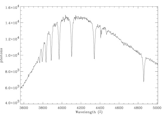
Figure 2: Typical spectrum of PG 1605+072 obtained at the Nordic Optical Telescope. The Balmer sequence is visible from H$\beta$ to H12, as well as the He i $\lambda$4471 Å line. The feature at $\sim$4410 Å is a bad CCD column.

Of all the known pulsating sdBs, PG 1605+072 has the most extreme properties, with the richest power spectrum (around 50 modes), the longest periods (up to $\sim$550 seconds), and the lowest surface gravity (log $g\sim\,5.25$) (?). The low gravity implies that the star may have evolved off the EHB; this hypothesis is supported by modelling by ? (?).

In Paper I (?) we reported the detection of Doppler variations in PG 1605+072. The dominant frequencies detected corresponded to those found in photometry (?), and we also found evidence of a wavelength dependence of the oscillation amplitude of the Balmer lines. In this paper we present new radial velocity observations covering a much longer time span. We do not confirm the wavelength dependence, but we do see evidence for very closely spaced frequencies, similar to the findings of ? (?). We also compare our results with those of ? (?), who observed this star with higher S/N and spectral dispersion, but over a much shorter time span (see Section 7). We will discuss equivalent width measurements from our spectra in a future paper.

2 Observations

The bulk of the observations were made on 11 nights over a 16-day period in May 2000 (see Table 2), using the DFOSC spectrograph on the Danish 1.54 m telescope at La Silla, Chile and the ALFOSC spectrograph mounted on the 2.56 m Nordic Optical Telescope on La Palma in the Canary Islands. To increase the frequency resolution of the amplitude spectrum and allow detection of very closely spaced oscillation modes, we also obtained observations at La Silla for about 1 hour per night in March–April 2000, before the main run (see Table LABEL:tab:marapr-obs).

Table 2: Spectroscopic observations of PG1605+072. LS = La Silla; NOT = Nordic Optical Telescope.

UT-date	Telescope	No. of	No. of
		hours	spectra
2000 May 11	Danish	6.87	370
2000 May 12	Danish	6.45	300
2000 May 16–17	NOT	7.31	337
2000 May 17–18	NOT	8.12	376
2000 May 18	Danish	6.75	319
2000 May 19	Danish	6.77	375
2000 May 19–20	NOT	8.40	473
2000 May 20	Danish	6.61	370
2000 May 21	Danish	2.69	146
2000 May 22	Danish	6.69	374
2000 May 23	Danish	6.67	369
2000 May 25	Danish	6.62	346
2000 May 26	Danish	1.24	70
Total		81.19	4225

The La Silla data (March to May) consisted of single-order spectra projected onto a 2K LORAL CCD. Pixel binning (to reduce readout noise) and windowing (to reduce readout time) gave 66 x 500-pixel spectra with a total wavelength range of 3650–5000 Å and a dispersion of 1.65 Å pixel^-1. The resolution was $\sim$6 Å, set by a slit width of 1.5 arcsec. The exposure time was 46 s, with a dead time of about 16 s. The average number of photons per Å in each spectrum was about 1700. A similar setup was used in previous observations (see Paper I).

The NOT data were similar, with 66 x 500 binned pixels covering a wavelength range of 3550–5000 Å. The dispersion was 1.65 Å pixel^-1 and the resolution was $\sim$8 Å, set by a slit width of 1.0 arcsec. The exposure time was 50–70 s, with a dead time of only 5 s. There was an average of about 8000 photons per Å in each frame. The data from both telescopes were timestamped in Modified Julian Date by the telescope computers to an accuracy of less than one second.

Figure 4: Velocity curve for H$\gamma$ from May 2000. No instrumental variation has been corrected for. There is a 3 day gap between the 2nd and 3rd panels from the top.

Table 4: Spectroscopic observations of PG1605+072 in March-April 2000.

UT-date	No. of	No. of
	hours	spectra
2000 March 18	0.30	12
2000 March 20	1.43	77
2000 March 21	0.45	25
2000 March 22	0.45	25
2000 March 23	0.57	32
2000 March 24	0.65	37
2000 March 25	0.72	41
2000 March 26	0.93	45
2000 March 27	0.93	52
2000 March 28	0.83	45
2000 March 29	1.17	59
2000 March 30	1.05	59
2000 March 31	1.07	59
2000 April 01	1.15	57
2000 April 04	1.03	65
2000 April 05	1.42	77
2000 April 06	1.47	80
2000 April 07	1.55	85
2000 April 08	1.65	90
2000 April 09	1.57	86
2000 April 10	1.70	95
2000 April 11	1.90	99
2000 April 12	1.23	65
Total	25.22	1367

3 Reductions

Bias subtraction, flat fielding and background light subtraction were done using IRAF, and 1D spectra were extracted using an Optimal Extraction algorithm (?). A cubic spline was fitted to the continuum level, and the spectra were normalised to a continuum value of unity.

The spectrum of PG1605+072 is dominated by Balmer lines (see Figure 2). Also present are some weak lines from He I (e.g, $\lambda$4471 and $\lambda$4922) and He II (e.g, $\lambda$4686). The Balmer lines are ideal to determine Doppler variations. A template spectrum was created by averaging 20 high-quality spectra from each night. By using a different template for each night, we are effectively applying a high-pass filter to the data.

To avoid pixelization effects in the cross correlation analysis, all spectra, including templates, were oversampled by a factor of 40 (using linear interpolation), and all but the Balmer line in question (one of H$\beta$, H$\gamma$, H$\delta$, H$\epsilon$ and H8) was cropped from each.

These spectra were modified further by subtracting 1.0 such that the continuum level was approximately zero. The result was passed through a half-cosine filter to smooth the transition to zero at the ends.

Each resulting template was then cross-correlated with its respective spectra to obtain pixel displacements. The velocities were obtained by using the known wavelengths of the Balmer lines to convert this displacement into wavelength and then Doppler shift. See Paper I for further details.

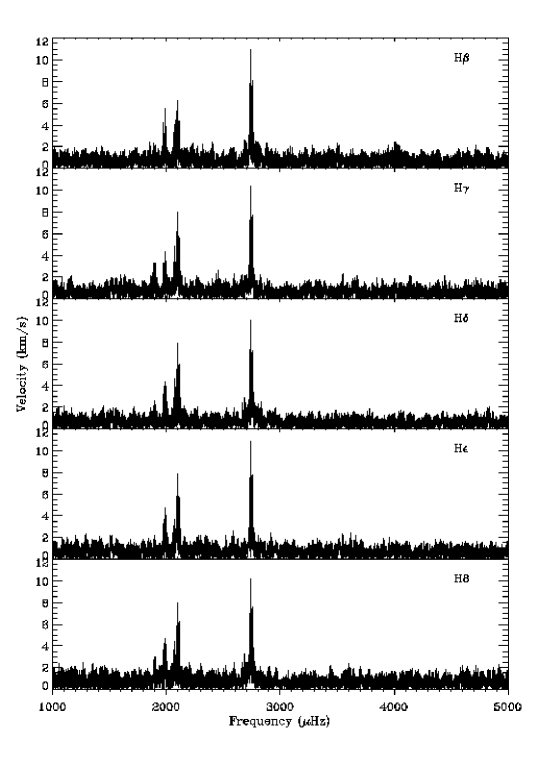
Figure 6: Amplitude spectra of five Balmer lines. No amplitude variation is evident in the dominant modes.

The velocity curve for H$\gamma$ is shown in Figure 4. It has not been corrected for slow instrument drifts. The high quality of the NOT data (3rd, 4th and 7th panels) – due to its larger aperture – suggests that fainter and/or shorter-period pulsating sdBs could be observed with this telescope.

4 Time-series Analysis

Because the quality of the observations varies through the data set, we performed frequency analysis using a weighted Fourier Transform (?), where weights were assigned to each night in the May 2000 data set according to the internal scatter. Weights for the March–April data were assigned to groups containing approximately the same number of observations as one night in the May data.

4.1 Velocities of Individual Balmer lines

The amplitude spectra of the five velocity time series from May 2000 are shown in Figure 6. There does not appear to be any substantial variation in velocity amplitude between the Balmer lines. We have analysed all five time series, using the non-linear least-squares multi-frequency fitting software Period98 (?). The frequencies found are shown in Table 6. The same technique was applied to the data presented in Paper I (July 1999) and these frequencies are shown in Table 8. White noise levels in the amplitude spectra are typically $\sim$1000 m s^-1 for each line in the July 1999 data, and 600–700 m s^-1 in the May 2000 data.

The major difference between the two sets of frequencies is the detection of the peaks at 1985 $\mu$Hz and 2075 $\mu$Hz in the May 2000 data set. In Paper I it was uncertain whether the non-detection of the latter (found to be the dominant mode in photometry by ? (? ? (?) in any of the individual Balmer line time-series, was due to variable amplitude or beating between closely spaced modes. With a slightly longer time-series and reduced noise, this mode is clearly detected in all Balmer lines. Somewhat surprising is the detection of the mode at 1985 $\mu$Hz, as this was found in photometry to have an amplitude of only 3.3 mmag, whereas the four other modes detected had amplitudes greater than 13.9 mmag. This mode may have variable amplitude or may be a series of unresolved modes. There is evidence for the latter possibility from ? (?), who found three modes around 1985 $\mu$Hz. As discussed further below, it is clear that the crowded frequency spectrum of PG 1605+072 severely complicates the interpretation of the observations.

In Paper I we reported the possible wavelength dependence of Balmer-line velocity amplitudes (see Figure 3 of that paper). Here, we have tried to confirm this result. Firstly, we found the weighted average frequencies of each of the four modes that were detected in all Balmer lines. These frequencies were then simultaneously fit to each time-series, giving amplitudes and phases for each mode.

Figure 8: Velocity amplitude as a function of wavelength. Diamonds represent the mode at 2742 $\mu$Hz, triangles for 2102 $\mu$Hz, squares for 2075 $\mu$Hz and crosses for 1985 $\mu$Hz. Small offsets to some points have been added in the wavelength direction to improve clarity. There is no clear dependence of amplitude on wavelength.

Figure 8 shows Balmer-line velocity amplitudes as a function of wavelength for these four modes. Error bars indicate the white noise level in the 3000–5000 $\mu$Hz region, where there appears to be no excess power. For three of the modes, there is no clear evidence for any wavelength dependence. For the 2102 $\mu$Hz mode (triangles), all lines except H$\beta$ appear to have the same amplitude, with the H$\beta$ amplitude being slightly lower. We do not feel this difference is significant enough to claim wavelength dependence, particularly as this peak may in fact be a combination of several closely spaced modes.

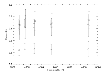
Figure 10: Oscillation phase as a function of wavelength. Symbols are the same as in Figure 8. Small horizontal offsets have been added for clarity.

Table 6: Frequencies (in $\mu$Hz) for five Balmer lines found from the May 2000 data.

H$\beta$	H$\gamma$	H$\delta$	H$\epsilon$	H8
	1891.26			1891.34
1985.73	1985.68	1985.58	1985.73	1985.79
2075.64	2075.72	2075.68	2075.68	2075.68
2102.21	2102.20	2102.17	2102.18	2102.24
2742.71	2742.68	2742.64	2742.70	2742.69

Table 8: Frequencies (in $\mu$Hz) for five Balmer lines found from the July 1999 data.

H$\beta$	H$\gamma$	H$\delta$	H$\epsilon$	H8
	1891.02	1891.00	1890.91
2102.14	2102.14	2102.11	2102.12	2102.12
2742.73	2742.47	2742.69	2742.67	2742.61

4.2 Combined Time-series

Figure 12: Amplitude spectra for July 1999 (top) and May 2000 (bottom) based on a combined Balmer line time series. Note the apparent change in amplitudes.

To reduce noise and perhaps detect more frequencies, we have combined the time-series for the five Balmer lines. Before doing this, we checked whether the oscillation phases were the same for each mode in each time-series. This is simply a matter of examining the phases found at fixed frequency. Relative phases are plotted as a function of wavelength for each mode in Figure 10, with errors determined using simple complex arithmetic (see ? (? ? (?). There is no evidence for phase variation with wavelength, leaving us free to combine the time series.

To do this, we simply averaged the velocity at each observation. This was possible since the weighting for each Balmer line was approximately the same. Weights were again derived from the internal scatter of each night. Combined time series were constructed, for both July 1999 and May 2000. The two resulting amplitude spectra are shown in Figure 12. There appears to be amplitude variation over the 10 month interval between the observations, which we discuss in Section 5. The white noise level is now 555 m s^-1 for the July 1999 data set and 425 m s^-1 for the May 2000 data set, an improvement of $\sim$45% over the best single-line amplitude spectra.

The fitted frequencies are shown in Table 10. The third column contains the differences in frequency between the two sets of data. The lengths of our two sets of observations are $\sim 7.9\times 10^{5}$ s (July 1999) and $\sim 1.3\times 10^{6}$ s (May 2000). If the formal frequency resolution is given by $1/T$, then the corresponding resolutions are $\sim$1.26 $\mu$Hz and $\sim$0.77 $\mu$Hz, respectively. Comparing these values with those in the third column of Table 10, we see that we have been able to estimate the frequency to much better than the formal resolution. In the final column we show the frequencies found from photometry, and again we see agreement that is better than the formal resolution. This is not surprising: at high signal-to-noise, the frequency of a strong peak in the power spectrum can be estimated to a precision many times better than the formal frequency resolution.

Table 10: Frequencies found after combining all Balmer lines in the July 1999 and May 2000 data sets. Note that $\Delta\nu=\nu_{2000}-\nu_{1999}$. The final column shows frequencies found by ? (?) for comparison.

$\nu_{2000}$	$\nu_{1999}$	$\Delta\nu$	? (?
($\mu$Hz)	($\mu$Hz)	($\mu$Hz)	(? (?)
1891.19	1890.98	$-$0.21	1891.42
1985.75	—	—	1985.32
2075.68	2075.29	$-$0.39	2075.76
2102.21	2102.15	$-$0.06	2101.65
2742.71	2742.63	$-$0.08	2742.72

4.3 Extended Time-series

To improve the frequency resolution still further, we now add the data from March–April 2000 (Table LABEL:tab:marapr-obs) to the May 2000 series. For the extended time-series ($T\sim 5.9\times 10^{6}$ s) the formal frequency resolution is $\sim$0.17 $\mu$Hz. The longer time-series does add complications however, since the number of alias peaks in the amplitude spectrum increases significantly. There is a gap of 45 days between the midpoints of the two time series, leading to aliasing that splits each peak into multiplets separated by $\sim$0.25 $\mu$Hz. The spectral window of each time series is shown in Figure 14. This includes the window function of all the 1999–2000 combined, which is discussed in Section 6. The extra aliasing is evident in the top two panels.

Figure 14: Spectral window (in amplitude) for 1999–2000, March–May 2000, March–April and May data sets in the range 2100-2105 $\mu$Hz. Alias peaks are seen in the top two panels with a $\sim$0.25 $\mu$Hz spacing, and in the top panel.

The frequencies and amplitudes determined from the extended (March–May 2000) time-series are shown in Table 12. The white noise level for this time-series is 370 m s^-1, and we use this as an error for the velocity amplitudes in column 3. The peaks at 2102 and 2742 $\mu$Hz, both shown as single in Tables 6 and 8, are now resolved into three and two peaks, respectively. Also shown are the differences in frequency when compared with photometry. If we take into account both our frequency resolution and the ambiguity from alias peaks, the frequencies we find are in excellent agreement with those found in photometry (?). In particular, the multiplicity of the peaks at 2102 and 2742 $\mu$Hz agrees with the extended time series ($T\sim$33 days) used by ? (?), who found 4 frequencies around 2102 $\mu$Hz and 4 around 2742 $\mu$Hz. They also found 5 frequencies around 2075 $\mu$Hz, 6 around 2270 $\mu$Hz, and 3 around 1985 $\mu$Hz. We have not detected these extra frequencies. It is not clear whether these multiple peaks are real or whether they caused by amplitude variability. We will for the moment consider them to be real, but will address this question in more detail in Section 5.

In Table 12, we note that the peaks at 2102.48 $\mu$Hz and 2765.09 $\mu$Hz are matched with quite low-amplitude modes found in photometry ($\sim$1 mmag), chosen because they are the closest in frequency. The latter frequency can also be identified with a higher amplitude mode detected by ? (?). We note also that 2765.09 $\mu$Hz is separated from $\sim$2742 $\mu$Hz by twice the one cycle per day alias frequency (i.e. 2$\times$11.57 $\mu$Hz). The mode at 2742.47 $\mu$Hz is also identified with a low amplitude mode, however it was only found in the extended time series of ? (?). Again, we have matched these modes purely because they are the closest in frequency. This appears to give further evidence for amplitude variability.

Table 12: 2000 frequencies, periods and amplitudes measured from the extended time-series. The fourth column shows the amplitudes found using the 2000 frequency solution, the fifth column shows the difference between the frequencies found in this paper and those found in photometry (?), and the sixth column shows photometric amplitude rank.

$\nu$	$P$	$V_{\mathrm{2000}}$	$V_{\mathrm{1999}}$	$\nu_{\mathrm{vel}}-\nu_{\mathrm{phot}}$	Rank
($\mu$Hz)	(s)	(km/s)	(km/s)	($\mu$Hz)	$n$
1891.01	528.82	1.99	3.18	$-$0.41	5
1985.75	503.59	4.13	0.63	+0.43	8
2075.72	481.76	4.27	2.11	$-$0.04	1
2101.57	475.83	3.40	4.97	$-$0.08	3
2102.48	475.63	8.47	11.1	+0.04	32
2102.83	475.55	3.66	3.05	$-$0.45	2
2269.84	440.56	1.75	0.90	$-$0.27	6
2742.47∗	364.63	4.45	3.57	$-$0.25	4∗
2742.85	364.58	7.17	2.87	+0.13	4
2765.09	361.65	1.97	0.29	$-$0.20	21

^∗This mode can also be identified as one of the extra frequencies found in an extended time-series in Table 4 of ? (?).

To further quantify this variability, we have fit the frequencies derived from the 2000 observations to our 1999 data. The amplitudes from the fit are shown in the fourth column of Table 12, next to the amplitudes from the 2000 observations for comparison. Errors in velocity are taken to be the white noise level (555 m s^-1). There are clearly large variations in most peaks (even more so, considering that the weakest 1999 amplitudes should be considered as upper limits).

Figure 16: Amplitude spectra for the Combined, March/April and May data sets in range 2100–2105 $\mu$Hz. The dashed lines indicated frequencies measured from the extended time series.

Figure 18: Same as Figure 16 expect in the range 2740–2745 $\mu$Hz.

Figure 20: Amplitude spectra of the 2100–2105 $\mu$Hz region showing the successive removal of 3 closely spaced frequencies.

5 Simulations

How well resolved are the closely spaced multiplets at 2102 $\mu$Hz and 2742 $\mu$Hz shown in Table 12? To answer this, we show the regions in question in Figures 16 and 18. From the top panel of Figure 16 it is clear that the frequency resolution is sufficient to resolve the power at 2102 $\mu$Hz into at least two peaks, perhaps three. The two frequencies found around 2742 $\mu$Hz also appear to be resolved in Figure 18. In the bottom panel of Figure 12 it appears that the peak around 2742 $\mu$Hz is higher than the one around 2102 $\mu$Hz, however Table 12 shows the opposite. This can be explained by examining the amplitude spectra (shown in Figure 20) around 2102 $\mu$Hz after each frequency is removed. It is still not clear, however, whether these frequencies are real or an artifact of the variation in amplitude of one frequency.

To investigate these effects further, we have created simulated time series for both our sets of observations (1999 and 2000). The inputs are the 10 frequencies measured from the time-series with the highest frequency resolution (i.e, 2000) with their corresponding amplitudes. Note that each simulation had exactly the same input amplitudes and frequencies, and only the phases were randomised. We have used two different noise levels, $\sim$600 m s^-1 and $\sim$300 m s^-1, as these bracket the noise in our observations. The same phases were used at both noise levels. The basic features of the two different groups of spectra are the same, implying that noise does not play a significant role in the shape of the amplitude spectrum. A selection of simulated amplitude spectra with noise $\sim$600 m s^-1 are shown in Figure 22 using the 2000 window function.

The most interesting feature of the majority of these spectra is the variability of the amplitudes of the peaks at $\sim$2102 $\mu$Hz and at $\sim$ 2742 $\mu$Hz. This observed variability does not depend strongly on the window function and arises from beating between the closely spaced modes around these two frequencies. However in Table 10 there is only a small difference ($<$0.1 $\mu$Hz) between frequencies measured in July 1999 and May 2000. If there were two or more frequencies beating, we would expect the peaks to move by more than this difference, since the measured frequencies span a range of $\sim$1.3 $\mu$Hz.

? (?) found 2 frequencies around 2102 $\mu$Hz in both halves of their $\sim$15 night time series, as well as in the full series. They also found weak “satellite” frequencies near almost all of the highest amplitude peaks. We find only one peak at 2102 $\mu$Hz in our May 2000 observations, however weighting the data may degrade the frequency resolution. The middle panel of Figure 16 suggests that 2 peaks may be clearly resolved in the March/April 2000 observations. If we assume there are 3 frequencies around 2102 $\mu$Hz, we detect 2 frequencies in $\sim$90% of our simulations. It seems that our detection of only one peak may be due simply to chance. Around 2742 $\mu$Hz only one frequency is always resolved, with the 2nd frequency resolved $\sim$50% of the time. This suggests a minimum of two frequencies around 2102 $\mu$Hz, and possibly two around 2742 $\mu$Hz. Two frequencies around 2742 $\mu$Hzis supported by ? (?), who finds a similar separation ($\sim$0.3 $\mu$Hz) in a re-analysis of the ? (?) observations. By combining all of our data (1999–2000), we are in a position to make one final test.

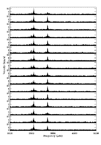
Figure 22: Simulated amplitude spectra using the 10 frequencies from Table 12 as input. These spectra are based on the window function of all observations from 2000. It is clear that the variable amplitude of the highest peaks is due to beating.

6 Combination of all observations

Figure 24: Same for Figure 20, except with combined 1999 and 2000 time series.

If we combine all of our observations (1999–2000), we find that the amplitudes of each peak is approximately the same ($\sim$8 km s^-1). This implies that the oscillations are coherent over this one year period, and we can therefore perform a frequency analysis on the time series. Combining all of the data introduces fine structure in the spectral window, as shown in the top panel of Figure 14 in the region around 2100 $\mu$Hz. The frequencies we measure from this time series are the same as those found in the March–May 2000 data, except around 2102.5 $\mu$Hz, where we now find 3 frequencies instead of two. These frequencies, while they describe the observations (see Figure 24), are split such that we consider them to be caused by amplitude variation. The two frequencies not found in 1999–2000, but found in the March–May 2000 data (2269.84 and 2765.09 $\mu$Hz), we consider marginal detections. We can now conclude that the frequencies in Table 14, derived from the March–May 2000 observations, are real.

Table 14: Detected frequencies and periods in velocities of PG 1605+072. These are based on the March–May 2000 observations, but also found in a time series of all observations (1999–2000).

Frequency ($\mu$Hz)	Period (s)
1891.01	528.82
1985.75	503.59
2075.72	481.76
2101.57	475.83
2102.48∗	475.63
2742.47	364.63
2742.85	364.58

^∗We include this frequency as representative of a mode with variable amplitude around 2102.5 $\mu$Hz.

7 Comparison with Woolf et al. (2002)

Our observations were by coincidence concurrent with those of ? (?), so we are in a position to examine some of their findings. Firstly, based on data taken over 16.3 hours across a 32.1 hour period, they found an apparent power shifting between modes, which we also find, and attribute to both amplitude variability over time and beating between closely spaced frequencies. They also found evidence for rotational splitting of the 2742 $\mu$Hz mode, and derived a rotational period of 12.6$\pm$2.8 hours. This is not in agreement with ? (?), who derived an upper limit on the rotational period of 8.7 hours from spectral analysis. While the pulsations cause some broadening of the spectral lines, the pulsation amplitudes are not high enough to shift ? (?’s upper limit into the range found by ? (? The rotational splitting they found is $\sim$11 $\mu$Hz, which is very close to one cycle per day. Because of this, the reality of this splitting should probably be treated with scepticism.

Some of our observations overlap with ? (?’s, and we have plotted in Figure 26 the amplitude spectrum of the two nights closest in time to theirs. Our observations for this period start at MJD 51675.1 and finish at MJD 51676.4, while the ? (? start at MJD 51675.9 and finish at MJD 51677.25. The dashed lines in the figure indicate the frequencies found by Woolf et al, which appear to be one cycle per day alias peaks. The dotted lines indicate the frequencies found in this paper. For comparison we have shown the spectral window of our observations in the top panel. The dashed lines correspond very well to the alias peaks in our spectral window, and we conclude that this is most likely what ? (? have identified, although the central peak (which we have identified with the frequency found in photometry) is not apparent in their amplitude spectra. We feel timing errors may be a possible explanation for the splitting, and lack of this central peak.

Figure 26: Amplitude spectrum of nights MJD 51675.1–51676.4 (bottom), showing no rotational splitting of the 2742 $\mu$Hz mode. The frequencies found by ? (?) are plotted as dashed lines. The peaks they correspond to are alias peaks. For comparison, the frequencies found in this work are plotted as dotted lines. The window function for the two nights (top) is also shown.

8 Discussion

The model of ? (?) is the best pulsation model for PG 1605+072 produced so far, although it only matches 5 of the dominant frequencies from ? (?) (they detected up to 55 frequencies, although some may be artifacts of amplitude variation). ? (?’s model predicts an equatorial velocity of $\sim$130 km s^-1 leading to a rotational period of around 3 hours, in agreement with the upper limit found by ? (?) of $P_{\mathrm{rot}}<8.7\mathrm{h}$ ($v$sin$i=39$ km s^-1).

What are the possible reasons for modes which are so closely spaced? Rotation has already been mentioned, however the minimum rotational splitting for an $l=1$ mode is $\sim$ 16 $\mu$Hz to first order, and for an $l=2$ mode is $\sim$ 27 $\mu$Hz. This is based on the maximum rotational period of ? (?), and assumes that the star oscillates in $g$-modes (?) in a similar way to a white dwarf. This is not the case, however, since unlike white dwarfs, horizontal motion does not dominate vertical motion on the surface of sdBs; in fact, they are of the same order (Kawaler, private communication). Despite this, the splitting values above are minima, so it is clear rotation is not the only effect causing splitting. Strong magnetic fields also cause splitting of oscillation modes, however little work has been done to measure fields of sdBs. Finally, we feel that amplitude variability over several months can explain at least some of the observed splittings. More detailed modelling of PG 1605+072 using the so-called second generation pulsating sdB models of ? (?) may help to answer these questions.

9 Conclusions

Of all the pulsating sdBs currently known, PG 1605+072 is clearly one of the most interesting. Using our newest observations we make several conclusions.

• From our main campaign we have detected 7 oscillation frequencies from velocity variations in the star. These frequencies are shown in Table 14. Most of these correspond to the strongest oscillation frequencies found in photometry.

• We find the velocity amplitudes and phases in the individual Balmer lines to be equal and cannot confirm the wavelength dependence of amplitude seen in Paper I.

• Apparent amplitude variability between our two sets of observations can be explained by a combination of beating between closely spaced modes and amplitude variability.

• To fully resolve and identify as many closely spaced frequencies as possible, it is necessary to have both good time coverage to reduce aliasing effects, and most importantly for PG 1605+072, to have a time series that is as long as possible, thus improving the frequency resolution in the amplitude spectrum.

• We can explain the possible rotational splitting of the 2742 $\mu$Hz peak claimed by ? (?) as an aliasing effect (possibly caused by incorrect time stamps), since our observations are concurrent.

PG 1605+072 offers asteroseismologists several challenges. It has many oscillation frequencies, although some have variable amplitudes; it has longer periods than most other pulsating sdBs, however it is rotating fast enough that rotationally split modes may be unequally spaced; it may be oscillating in $p$ or $g$-modes or a combination of both. Further theoretical work is needed in these areas. We feel that despite these challenges, a campaign of simultaneous photometry and spectroscopy will help to answer the questions we have raised here, and perhaps allow us to comprehend one of the least understood phases of stellar evolution.

The authors would like to thank Steve Kawaler for helpful discussions. This work was supported by an Australian Postgraduate Award (SJOT), the Australian Research Council, the Danish National Science Research Council through its Center for Ground-based Observational Astronomy, and the Danish National Research Foundation through its establishment of the Theoretical Astrophysics Center.