Point source detection and extraction from simulated
Planck TOD using optimal adaptive filters

Abstract

Wavelet-related techniques have proven useful in the processing and analysis of one and two dimensional data sets (spectra in the former case, images in the latter). In this work we apply adaptive filters, introduced in a previous work (Sanz et al. 2001), to optimize the detection and extraction of point sources from a one-dimensional array of time-ordered data such as the one that will be produced by the future 30 GHz LFI28 channel of the ESA Planck mission. At a $4\sigma$ detection level 224 sources over a flux of 0.88 Jy are detected with a mean relative error (in absolute value) of $21\%$ and a systematic bias of $-7.7\%$. The position of the sources in the sky is determined with errors inferior to the size of the pixel. The catalogue of detected sources is complete at fluxes $\geq$ 4.3 Jy. The number of spurious detections is less than a $10\%$ of the true detections. We compared the results with the ones obtained by filtering with a Gaussian filter and a Mexican Hat Wavelet of width equal to the scale of the sources. The adaptive filter outperforms the other filters in all considered cases. We conclude that optimal adaptive filters are well suited to detect and extract sources with a given profile embedded in a background of known statistical properties. In the Planck case, they could be useful to obtain a real-time preliminary catalogue of extragalactic sources, which would have a great scientific interest, e. g. for follow-up observations.

1 Introduction

One of the most thrilling challenges in the study of the Cosmic Microwave Background (CMB) is to deal with the problem of separating the cosmological signal from the different foregrounds and noises that appear in CMB experiments. This problem will be specially relevant in future high-resolution experiments such as MAP (Bennett et al. 1996) and Planck (Mandolesi et al. 1998, Puget et al. 1998). From the point of view of determining constraints on fundamental cosmological parameters, the different foregrounds (synchrotron emission, galactic dust, free-free radiation, thermal and kinetic Sunyaev-Zel’dovich (SZ) emission from galaxy clusters and extragalactic point sources) are considered as contaminants and therefore must be removed together with the noise in order to extract the cosmological signal. Besides, knowledge about each of these ’contaminants’ has a great scientific relevance on itself. Therefore, it is of exceptional importance to be provided with good techniques of denoising and foreground separation.

There are several methods already available to perform the separation of the different components in CMB observations, such as the ones based on Wiener filter (Tegmark and Efstathiou 1996, Bouchet and Gispert 1999) and on Maximum Entropy Methods (MEM, Hobson et al. 1998, 1999; Stolyarov et al. 2001). All these methods take advantage of the different statistical properties of the CMB and the foregrounds (e.g. different angular power spectra) as well as the knowledge of their distinctive frequency dependence. When neither the spatial distribution of the foregrounds nor its frequency dependence are well known the performance of these separation methods dramatically drops. Such is the case of point sources, whose spatial distribution and abundance remains uncertain and whose frequency dependence is not well known. Besides, they can show temporal and even spectral variability. Extragalactic point sources should be removed from the maps before any analysis should be performed. Maximum Entropy Methods can produce a catalogue of point sources as a residual (noise) from the separation process. However, only the faintest sources are recovered, and the brightest ones can still be observed in the residuals. The Independent Component Analysis technique (Baccigalupi et al 2000, Maino et al 2001) has also been applied to this problem with promising results: it has the advantage that, unlike the previous methods, it does not need any prior knowledge of the components to be separated, but its weakest point is actually the separation of point sources.

Filtering techniques have been successful in both denoising and extracting the brightest point sources from CMB maps. Tegmark and Oliveira-Costa 1998 presented a filtering scheme that minimizes the variance of the map. However, their filter does not produce a maximum gain (considered as the ratio between the $\sigma$-level of the source after filtering and the $\sigma$-level of the source before filtering) at the scale of the source. All the point sources in a CMB map will have the same profile and size (the convolution of a $\delta$-Dirac source with the antenna beam) and the filtering process should take advantage of this fact using a filter optimal for that particular profile and size (scale). Wavelet techniques are specially suitable to deal with scales and spatial location at the same time. The application of the Mexican Hat Wavelet (MHW) to realistic simulations was presented in Cayón et al. (2000) and extended in Vielva et al. (2000a). The principal advantage of this method is that no specific assumptions about the statistical properties of the point source population or the underlying emission from the CMB and other foregrounds is required. The MHW and MEM techniques have successfully been combined to extract both faint and bright point sources at the same time (Vielva et al. 2000b).

It is desirable to exploit to the maximum the mentioned scale distinctiveness of point sources. In Sanz et al. 2001 (S01, hereafter), a method was presented to, for a given source brightness profile and given the statistical properties of the background (CMB plus foregrounds and noise), derive the analytic shape of the optimal filter for the particular considered case. That kind of filter was called ’optimal pseudo-filter’. S01 defines as an optimal pseudo-filter one that a) is unbiased, b) gives a maximum at the position and scale of the source and c) gives the minimum variance of pseudo-filter coefficients (i.e. is an efficient estimator of the amplitude of the sources) under assumptions a) and b). They considered one, two and three-dimensional cases and showed that the MHW is optimal (in the mentioned sense) or nearly optimal for a two-dimensional Gaussian profile and reasonable foreground conditions. After carefully thinking about the terminology used in that previous work, we have decided to substitute the rather confusing ’pseudo-filter’ term by ’adaptive filter’. This is so because a filter that satisfies conditions a) to c) adapts itself to the characteristics of the signal and the noise. In the following we will use ’adaptive filter’ in the same sense as ’pseudo-filter’ in S01.

Although two-dimensional maps are the most useful and extended form to show CMB data, they are only available after an exhaustive process of analysis and reduction of the raw data from CMB experiments. These experiments scan different patches of the sky in a sequence producing a unidimensional set of time ordered data (TOD). TODs suffer from lower signal-to-noise ratios than final two-dimensional maps, but on the other hand are less likely to show artifacts coming from the data reduction, such as pixel-to-pixel noise correlations. Moreover, TODs can be analyzed in (almost) real time during the observations in order to produce early (preliminary) catalogs of sources.

In this paper we apply the techniques developed in S01 to realistic simulations of the TOD coming from one of the 30GHz Planck LFI’s channels. In section 2 we summarize some of the conclusions of S01 and present the semi-analytic adaptive filter that should be used in a realistic case. Section 3 describes the simulations used in this work. In section 4 we describe the analysis of the simulated data. In section 5 we describe the performance of the optimal adaptive filter, comparing it with other filtering schemes such as Gaussian filter and MHW. Finally, in section 6 we discuss our conclusions and give an outline of future work in this field.

2 One-dimensional adaptive filter

The general formalism of adaptive filters in an n-dimensional image was presented in S01. TODs can be considered as a particular case of a one-dimensional image (a spectrum is another interesting case). The image data values can be expressed as

$$y(t)=s(t)+n(t),$$ (1)

where $t$ is the time, $s(t)$ represents a symmetric source and $n(t)$ is a homogeneous and isotropic background with mean value $<n(t)>\,=0$ and characterized by the power spectrum $P(q)$ ($q$ is the absolute value of the ’wave vector’ associated to $t$). If $A=s(0)$ is the amplitude of the source we can introduce the profile $\tau(t)$ as $s(t)=A\tau(t)$. Let us introduce a centrally symmetric adaptive filter $\Psi(t;b,R)$

$$\Psi(t,b,R)=\frac{1}{R}\psi(\frac{|t-b|}{R})$$ (2)

where $b$ defines a translation whereas $R$ defines a scaling. The adaptive filtered field is defined as:

$$w(R,b)=\int dt\,y(t)\Psi(t;b,R)\equiv\int dq\,e^{-iqt}y(q)\psi(Rq)$$ (3)

In the last equivalence we have expressed the convolution as a product in Fourier space.

Following S01, it is possible to derive the analytic form of the optimal adaptive filter for a given source profile, once we have defined what we mean by ’optimal’. Let us define an optimal adaptive filter as one that satisfies the following conditions:

1. There exists a scale $R_{o}$ such that at the point source position ($b=0$) $<w(R,0)>$ has a maximum at that scale.

2. $<w(R_{o},0)>=s(0)$, i.e. $w(R_{o},0)$ is an unbiased estimator of the amplitude of the source.

3. The variance of $w(R,b)$ has a minimum at the scale $R_{o}$, i.e. we have an efficient estimator.

Given these three conditions, the solution (adaptive filter) is found to be:

$$\tilde{\psi}(q)\equiv\psi(R_{o}q)=\frac{\tau(q)}{2P(q)\Delta}[b+c-(a+b)\frac{d\ln\tau}{d\ln q}]$$ (4)

$$a\equiv\int dq\frac{\tau^{2}}{P},\ \ b\equiv\int dq\frac{\tau}{P}\frac{d\tau}{d\ln q},$$

$$c\equiv\int dq\frac{1}{P}[\frac{d\tau}{d\ln q}]^{2},\ \ \Delta=ac-b^{2}$$ (5)

The limits of the integrals go from $0$ to $\infty$.

In S01 analytic expressions for Gaussian sources and backgrounds of the type $P(q)\propto q^{-\gamma}$ were derived. In a more realistic case, the background can not be modelled in such a simple way, and integrals in (2) should be numerically estimated. When dealing with real data (or realistic simulations such as those used in this work) we must perform the following steps: first, determine the power spectrum of the background directly from the image. Second, evaluate integrals (2). Third, build the adaptive filter (4) and make the convolution (3). Finally, we can proceed to detect the sources, for example looking for peaks above a certain $\sigma$-level in the coefficient (filtered) image.

When determining the power spectrum of an image we obtain the power spectrum of both the background and the sources together. In the following we consider that the contribution of the point sources to the total power spectrum is negligible. This is a reasonable assumption in a realistic case, specially at medium and high wavelengths where the emission of IR and radio sources is weak. Another problem related to power spectrum determination is the variance of the power spectrum estimator. The variance of one-dimensional power spectrum estimators tends to be larger than that of two-dimensional cases because the number of sample points is usually smaller. A possible solution to this problem is to estimate low resolution power spectra. However, a large amount of information is lost at scales that are crucial for the determination of the adaptive filters. For this work we chose to average the estimated power spectra of adjacent rings of the TOD (corresponding to regions of the sky separated by only a few arcminutes and therefore possessing very similar underlying power spectra).

A typical profile of the optimal adaptive filter (in Fourier space) for a section of the simulated TOD used in this paper is shown in figure 1. The profile (solid line) is irregular due to the roughness of the estimated power spectrum. These irregularities reflect the particularities of the data and define the scales where the adaptive filter is more or less efficient. For comparison, a Mexican Hat Wavelet (dashed line) and a Gaussian (dotted line), both of them with a width equal to the width of the source, are also shown.

Figure 1: Several filters in Fourier space. The optimal adaptive filter particularised for an individual ring of our simulations is represented by a solid line. The dashed line shows a Mexican Hat Wavelet of width equal to the width of the (Gaussian) source. The dotted line represents a Gaussian of width equal to the width of the source. All filters are normalized to give the true amplitude of the source after convolution.

3 Data

For this work we chose the 30 GHz LFI28 channel of Planck because of the relatively small size of its resulting TOD. Higher frequencies, in spite of being expected to show more contribution from point sources due to their higher resolution and the contribution of IR sources at $\nu\geq 300$ GHz, lead to huge TOD sets and require many hours of computation to be simulated and analysed on an average computer and will be analyzed in a future work.

Our data simulates a 6 months run of the 30 GHz LFI28 channel of Planck, covering the whole sky except for two circles of $1\degr 82$ around the ecliptic poles. The sky simulation consist of the addition (in flux) of a CMB simulation and three templates, each for the Galactic synchrotron radiation, Galactic dust and thermal SZ. These templates have been generated using proper models that are freely distributed among the Planck collaboration. This sky is then combined with a map of point sources, generated from a catalog performed following the model of Toffolatti et al. 1998 (that is not public for the Planck collaboration) and then ’observed’ by the Planck Pipeline Simulator for one of the LFI 30 GHz radiometers; resulting in a TOD for the observed sky (CMB, foregrounds and point sources) plus instrumental noise. The data are ordered in circular rings centered on points situated on the Ecliptic. The angle between the pointing axis and the rotation axis for the LFI28 instrument is $88\degr 18$. The maximum separation between two consecutive rings is $2.5\arcmin$ (at the intersection with the Ecliptic plane). Each ring results from the average of 60 revolutions of the detector around the rotation axis, corresponding to one hour of integration time, and contains 1950 measures of antenna temperature. There are a total of 4383 of such rings, leading to 8546850 measures of temperature. The antenna has a FWHM of $33\arcmin$ and its response slightly differs from a circular Gaussian one.

The simulation contains CMB emission, different extended foregrounds (Galactic synchrotron, dust and free-free, thermal and kinetic SZ emission from clusters, etc), point sources and instrumental noise. Both white noise and $1/f$ noise are present. The knee frequency $f_{\nu}$ is set to be $<20$ mHz (less than the frequency of rotation). In the lower panel of figure 2 we show a segment of one of the rings of the simulation. There is a bright point source near pixel 400 (in fact, it is the brightest source in the simulation). Apart from this extraordinarily bright source, the features that dominate the image are Galactic emission (the large peaks around pixels 150 and 940) and noise.

4 Data analysis

The complete set of simulated TOD was filtered using the optimal adaptive filter described in section 3. Each individual ring was filtered separately. The power spectrum that appears in equations (4) and (2) was obtained by averaging the estimated power spectra of twenty-one consecutive rings (the ring that is being filtered, the ten previous rings and the ten subsequent rings).

Figure 2: A 1024-pixel section of one of the rings before and after filtering. The lowest panel shows the section before any filtering. The second panel shows the section after filtering with a Gaussian of FWHM $33\arcmin$ (equal to the one of the source). The third panel shows the section after filtering with a Mexican Hat Wavelet of width equal to the width of the source. The top panel shows the section after filtering with the optimal adaptive filter.

In order to detect the sources from the filtered image one can set a certain threshold over the dispersion of the filtered ring and look for connected regions (peaks) above that threshold. That would be the most direct detection method if the different rings were independent of their neighbours. This is not the case, since adjacent rings scan very close regions and each source is expected to appear in more than one ring. The use of information coming from neighbouring rings allows to increase the effective signal to noise ratio of the detections and to discard spurious ’sources’ due to noise fluctuations. The most straightforward way to detect sources is then to perform a kind of two-dimensional thresholding, looking for connected pixels at equal latitude that appear in several adjacent rings. In a first approximation, the position of the source will be the position of the maximum of that region of connected pixels. We will show that this approximation is good enough for the purpose of locating the sources with an error comparable to $1/3$ of the antenna FWHM.

Two different regimes of ’noise’ have to be removed in order to optimize the detection of the sources. The large scale features due to Galaxy foregrounds as well as CMB fluctuations are strongly correlated between a given ring of data and its neighbours. On the other hand, the small scale noise, dominated by white instrumental noise, is expected to be nearly independent from one ring to another. This suggests a further step in the idea of combining information from nearby rings to increase the signal to noise ratio of the sources. By averaging each ring data (before filtering) we can construct a ’synthetic TOD’ in which the large scale fluctuations are almost the same than in the original TOD but the noise at the scale of the pixel has been greatly diminished. The $1/f$ will still be present in the averaged TOD. The point sources of the original TOD are replaced in the averaged TOD by Gaussians of amplitude

$$A_{a}=\frac{1}{N_{a}}\sum_{i=1}^{N_{a}}Ae^{-\frac{\mid\vec{x_{o}}-\vec{x_{i}}\mid^{2}}{2\sigma_{b}^{2}}}$$ (6)

where $A$ is the true amplitude of the source, $N_{a}$ is the number of rings that are averaged, $\sigma_{b}$ is the beam width and the distance $\mid\vec{x_{o}}-\vec{x_{i}}\mid^{2}$ is the geodesic (spherical) angular distance between the pixel corresponding to the position of the source and the pixel that is being added to calculate the average. This is true when the beam is a perfect Gaussian because in that case the average is a weighted sum of Gaussians of equal width, that is, a new Gaussian of the same width and amplitude given by eq. (6). Therefore, we can filter the rather denoised, ’synthetic TOD’, instead of the original TOD and correct the amplitude of the sources that we will detect using eq. (6) in order to recover an estimate $\hat{A}$ of the true amplitude $A$.

Although the Planck Pipeline Simulator uses a realistic beam, we assumed for this work that the beam is a perfect Gaussian. In section 5 it will be shown that this approximation works reasonably well. However, future work should take into account real beams; the 30 GHz detector is expected to be slightly elliptic. This asymmetry will introduce complicate effects in the map making and analysis. In the case of TOD the effect of ellipticity, when projected over the scan trajectory, is a change in the ‘effective width’ of the beam. Therefore, the scale-adaptive filter should be calculated for such ‘effective width’. More complicated asymmetries will require more careful treatment. Future work will deal with this issue.

5 Results

In order to determine the goodness of the averaging of close rings we performed two different filterings of the TOD. In the first case, the raw data of the TOD were filtered ring by ring as described in the section 4. In the second case, a ’synthetic TOD’ in which each individual ring was the average of the original ring (at that position) with the twelve neighbours was constructed. The number of rings averaged is such that at the maximum ring spatial separation region on the sky (the ecliptic Equator) the separation between the two most separated rings is approximately equal to the FWHM of the beam. After filtering, the detection and extraction was performed looking for sets of 5 or more connected pixels (in the 2-dimensional sense). A lesser number of connected pixels required would lead to a much higher number of spurious detections. To check if the detections correspond to real sources we compare with the catalogue of the 1000 brightest sources present in the simulations. This catalogue is complete and its flux limit is clearly lower than the expected flux limit of the detected sources.

In the lower panel of figure 3 the number of detections (defined as the number of peaks encountered above a certain threshold that correspond to a real source in the reference catalog) above several $\sigma$ thresholds is shown for the case where the data have been averaged (filled circles and solid line) and the case where they have not (open circles and dashed line). The remaining quantities of interest (such as estimation of the amplitudes, fluxes, etc.) concerning the detection/extraction of sources over the averaged and then filtered TOD are shown in table 1 and will be discussed later. As expected, the number of sources detected when analysing the synthetic TOD is 4 to 5 times higher to the number of sources detected over the original, filtered TOD for every $\sigma$ level.

Table 1: Detections at 30GHz with the Optimal Adaptive filter, compared to a Mexican Hat Wavelet (MHW) and a Gaussian window with FWHM of $33\arcmin$. Col. (1): $\sigma$ detection level. Col. (2): Number of sources found. Col. (3): Number of spurious detections. Col. (4): Mean position offset. Col. (5): Mean relative absolute error of the amplitude (defined as $r.a.e.=\mid A_{0}-A_{e}\mid/A_{0}$, where $A_{e}$ is the estimated amplitude). Col. (6): Mean bias in the amplitude. Col. (7): Minimum reached flux. Col. (8): Flux over which the catalog of detections is complete.

$\sigma$	detected	spurious	mean offset	m.r.a.e.	$<bias>$	min. flux	compl. flux
	sources	sources	($\arcmin$)	($\%$)	($\%$)	(Jy)	(Jy)
Optimal Adaptive filter
2.5	549	1368	14.08	24.22	3.15	0.542	4.337
3.0	403	296	13.56	24.32	1.31	0.644	4.337
3.5	351	54	12.73	21.75	-4.91	0.760	4.337
4.0	224	22	12.49	20.98	-7.69	0.885	4.337
5.0	150	9	12.20	19.82	-14.85	1.065	4.337
5.5	124	5	12.03	20.38	-15.54	1.197	4.337
Gaussian filter
2.5	11	11	18.88	538.4	537.0	6.511	17.070
3.0	7	6	17.84	746.4	744.2	8.787	10.070
3.5	7	13	17.50	898.1	898.1	7.908	18.866
4.0	4	11	17.24	1281.7	1281.7	10.340	18.866
5.0	4	12	13.09	1985.3	1985.3	13.926	18.866
5.5	4	15	13.09	1985.3	1985.3	13.926	18.866
Mexican Hat Wavelet
2.5	473	413	12.83	21.46	4.27	0.531	4.337
3.0	361	130	12.66	20.76	2.52	0.693	4.337
3.5	270	63	12.67	20.46	0.45	0.761	4.337
4.0	196	59	12.40	18.47	-4.22	0.844	4.337
5.0	139	49	12.50	19.47	-4.96	0.957	4.337
5.5	118	44	12.41	19.83	-5.53	1.099	4.337

Apart from having the greatest number of detections, it is also of great importance to reduce as much as possible the number of spurious detections. In the lower panel of figure 4 (labeled as ’simple detection’) the ratio between spurious and ’true’ detections is represented for the case where the data have been averaged (filled circles and solid line) and the case where they have not (open circles and dashed line). The ratio is lower for the case in which the data have not been averaged. It is evident that a kind of compromise has to be reached between gain and reliability. If we arbitrarily set a maximum proportion of spurious sources versus true ones, say a $10\%$ (represented in fig. 4 with an horizontal dashed line), we can determine the minimum $\sigma$ level that satisfies this condition. In this example, for the case of non-averaged rings, we can reach the $3\sigma$ and find 80 sources (to a minimum flux of 4.33 Jy) with a $7.5\%$ of spurious detections. For the case of averaged rings, we must go to the $4\sigma$ level, where we find 224 sources (to a minimum flux of 0.885 Jy) with a $9.8\%$ of spurious detections. We conclude that the averaging of neighbouring rings is a valid strategy to reduce pixel-scale noise. In the following, all the results will refer to filtering of averaged rings.

The number of detections and spurious sources found with the optimal adaptive filter applied to a synthetic TOD is shown in table 1. The determination of the position of the source, the mean relative absolute error in the determination of the amplitude (defined as $m.r.a.e.=\mid A_{0}-A_{e}\mid/A_{0}$, where $A_{e}$ is the estimated amplitude and $A_{0}$ is the real amplitude), the mean bias (defined in the same way as the m.r.a.e, but without the absolute value), the minimum flux reached and the completeness flux are also included in table 1. In each case the mean error in the position of the sources is comparable with the size of the ’pixel’ of the TOD, $11\arcmin$. The determination of the amplitude using eq. (6) has relative errors ranging from $24.32\%$ at $3\sigma$ threshold to $19.82\%$ at $5.0\sigma$. The error decreases as the detection threshold increases. This indicates that the estimation of the amplitude of weak sources is less accurate than the estimation of the amplitude of bright ones. Also, the determination of the amplitude is biased to higher values at low $\sigma$ levels and to lower values (negative bias) at high $\sigma$ levels. The positive bias for weak sources arises due to the peak finding algorithm: it finds preferently the maxima in pixels where the noise contribution is positive.

Let us consider for a while the possible causes for the mentioned bias and how to deal with it. Scale-adaptive filter is designed to be an unbiased estimator of the amplitude of the sources. Thus, the method is unbiased. However, in practise it is found a small bias. The origin of this bias can be found in two different kind of effects. On the one hand, the bias introduced by the detection method: this bias was described in the last paragraph and is related with the well-known ‘detection bias’. On the other hand, bias may arise due to the non-ideality of the data. In first place, the profiles considered in the design of the filters are continuous whereas real data is pixelised. Therefore, the correlation between the (continuous) filter and the (pixelised) source profile is not perfect, this resulting in a non-ideal performance of the filter. In second place, the limits in the integrals (2) are from $0$ to $\infty$, whereas in real data the frequencies are limited by the sizes of the data set and the pixel. Therefore, integrals (2) can only be approximately calculated. This leads to an inaccuracy in the determination of the shape of the filter and, more important for the bias, the normalization (the $\Delta$ in the mentioned integrals). Another source of bias appears when the assumption about the profile of the sources is wrong. For example, we have assumed that the detector beam is Gaussian, while in fact it is not; this could explain the bias in our results. In SO1 it was found using simple simulations that the bias due to the non-ideality of the data was negative. Similarly, the negative bias that appear here is interpreted in the way described above. In practise, it is difficult to distinguish from the data the different contributions to the bias among the ones above mentioned. A possibility to overcome the bias is to calibrate it using a great number of simulations with the same background and artificial sources of known amplitude. Once removed the ‘systematic’ bias, the remaining error will be statistical. This kind of study will be carried on in a future work.

In the case we are considering the bias is never greater than $16\%$. At intermediate thresholds, the (positive) effects of detection bias and the non-ideality of the data (negative) tend to cancel and, on average, the amplitude estimates are unbiased. To compare with other ’classical’ filters we repeated the process using a Gaussian filter and a Mexican Hat Wavelet (MHW, hereafter), both of them with a width equal to the beam width of the antenna ($33\arcmin$). The normalization of both filters was chosen so that the coefficient at the position of the source is equal to the amplitude of the source (that is, the filtering process does not change the amplitude of the sources). The adaptive filter automatically satisfies this condition (condition 2 for an optimal adaptive filter). While the MHW and the optimal adaptive filters are both band-pass filters, the Gaussian is a low-pass filter, so the comparison with the Gaussian is a bit unfair: the Gaussian is expected to perform significantly worse than the other two filters. The number of detections above several thresholds for the two ’classical’ filters together with the optimal adaptive filter are shown in table 1. The number of detections is similar for the MHW and the optimal adaptive filter, yet are slightly higher for the optimal adaptive filter. The lowest number of detections corresponds to the Gaussian filter. In the lower panel of figure 5 the number of detections with the three different filters is compared. Detections with the optimal adaptive filter are shown with open circles and solid line. The open boxes and dashed line corresponds to MHW detections and the triangles and dashed line corresponds to Gaussian filter detections. The ratio between spurious and true detections for the three filters is shown in the top panel of figure 5. Except for the $2.5\sigma$ level, the Gaussian filter produces the worst ratio. The optimal adaptive filter gives spurious to detected ($e/d$) ratios that quickly decline with increasing $\sigma$ thresholds. The $e/d$ ratio for the MHW remains almost constant with $\sigma$ in the considered cases and clearly exceeds the ratio obtained with the optimal adaptive filter. The m.r.a.e. and the bias in the determination of the amplitude are huge in the case of the Gaussian filter. Both have very similar values. That means that the main source of error is systematic (the filter is biased). Considering the m.r.a.e, the MHW seems to give amplitude estimates a few percent better than the optimal adaptive filter. Flux limits are similar in the MHW and optimal adaptive filter cases. The Gaussian filter leads to higher inferior flux and completeness limits.

Figure 2 provides a useful insight into what is happening with the different filters. The Gaussian filter smoothes the image, removing very efficiently the small scale noise but allowing the large structures (the Galaxy and others extended fluctuations) to remain in the image. The naive $\sigma$ thresholding counts these bright, large structures as sources, leading to a big relative number of spurious detections. Besides, the sources that by chance lie on ’valleys’ of the background can not be detected. On the other hand, sources that lie on areas of positive background are enhanced and can be more easily detected. This can explain the large and positive bias in the detections with the Gaussian filter.

Both MHW and optimal adaptive filter are better prepared to deal with this problem than the Gaussian window. Their profiles in Fourier space drop to zero at low frequencies and thus they are efficient in removing large scale structures. Images filtered with the MHW and the optimal adaptive filter in figure 2 are similar. A visual inspection reveals that MHW smoothes better the high-frequency fluctuations. The optimal adaptive filter is more efficient in removing medium and large structures. The fluctuations around pixel 150 (corresponding to one of the two observations of the Galaxy in the ring) are better removed with the optimal adaptive filter than with the MHW. This is more apparent in figure 1 where the profiles of the different filters in Fourier space clearly indicate the faster drop of the adaptive filter at low frequencies (large scales) and its slower drop at high frequencies (small scales). The MHW can have the same problem as the Gaussian filter. However, the probability of this problem should be smaller due to its better efficiency in removing the Galaxy and other large-scale structures. This effect explains the higher $e/d$ ratio and the trend to positive bias.

We conclude that the optimal adaptive filter detects point sources better than the MHW and the Gaussian window. The number of detections is comparable to the number of detections with the MHW and clearly higher than with the Gaussian window. The relative number of spurious detections with the optimal adaptive filter is lower, except for very low detection thresholds, than with the MHW and the Gaussian window. Over $4\sigma$ the contamination of spurious detections is lower than $10\%$. At this level ($4\sigma$) the number of expected sources in all the sky is of a few hundreds (224 in our simulation) above fluxes of around 0.9 Jy.

Figure 3: 30 GHz detections with the optimal adaptive filter as a function of the $\sigma$ detection threshold. The open circles and dashed lines represent detections over the filtered TOD. The filled circles and solid line represent detections over a filtered synthetic TOD in which each ring is the result of the average of 9 rings of the original TOD. The synthetic TOD has the same number of rings than the original one. Two cases have been represented: simple detection over a certain threshold (lower panel) and simple detection excluding a $5\deg$ band around the Galactic plane (top panel).

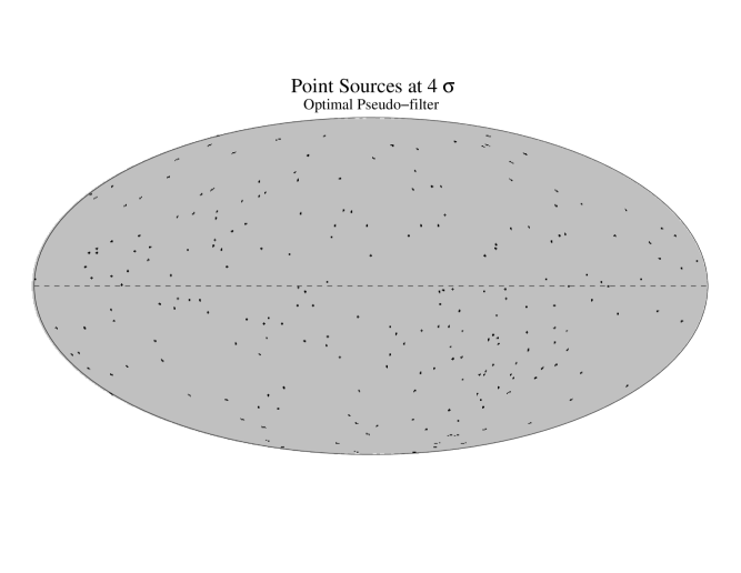
Figure 6: Positions of the detected sources with the optimal adaptive filter at a $4\sigma$ detection level. The sky is projected in Galactic coordinates. The dashed line represents the Galactic Equator. The optimal adaptive filter is able to detect sources even in the highly contaminated region around the Galactic Plane.

Some tests can be performed in order to discover if the number of spurious sources, the most unpleasant effect of the filtering and detection process, can be reduced. Where do these spurious detections come from? One possibility is that the peak finding algorithm is detecting the Galaxy or other large-scale features. Such structure will appear in several adjacent rings, as sources do, and therefore a possibility of confusion exists. To test this potential source of contamination, we repeated the analysis excluding a band of $5\deg$ centered on the Galactic plane (corresponding to a $4.36\%$ of the sky area). The top panels of figures 3 and 4 show the number of detections and the ratio of spurious/true detections, respectively, for the optimal adaptive filter in the cases where the rings have been averaged (as explained before, filled circles) and where they have not (open circles). In the first section of table 2 are the results for the case of averaged rings (the tabulated quantities are the same than in table 1) are shown. The decrease in the number of detections corresponds to the one expected for a uniform distribution of sources in the sky (around $5\%$). This indicates that the density of detections around the Galactic plane is not substantially different from the density of detections in other regions, less ’contaminated’, of the sky. This can be seen in figure 6, where the $4\sigma$ detections have been represented in Galactic coordinates (the Galactic Plane being represented by a dashed line).

Figure 4: 30 GHz ratio between the number of spurious sources and the number of true detections with the optimal adaptive filter as a function of the $\sigma$ detection threshold. The open circles and dashed lines represent detections over the filtered TOD. The filled circles and solid line represent detections over a filtered synthetic TOD in which each ring is the result of the average of 9 rings of the original TOD. The synthetic TOD has the same number of rings than the original one. Two cases have been represented: simple detection over a certain threshold (lower panel) and simple detection excluding a $5\deg$ band around the Galactic plane (top panel).

The ratio between spurious and true detections remains almost untouched for low $\sigma$. For higher $\sigma$ levels, the proportion of spurious detections that are due to the Galactic plane increases dramatically (comparing tables 1 and 2 we see that this proportion increases from a $7\%$ at $2.5\sigma$ to a $89\%$ at $5\sigma$). This indicates that the contamination by the Galaxy dominates at high signal to noise ratios, whereas low-intensity contamination is dominated by noise fluctuations. In all cases, the number of peaks that correspond to the Galaxy is much smaller than the number of detected sources, thus implying that the optimal adaptive filter deals efficiently with large scale backgrounds.

Table 2: Different tests for the detections at 30 GHz. Columns have the same meaning than in table 1. Two different cases are tabulated: detections with the optimal adaptive filter when a $5\deg$ band around the Galactic plane is excluded from the analysis and detections with a $33\arcmin$ MHW when a $5\deg$ band around the Galactic plane is excluded from the analysis.

$\sigma$	detected	spurious	mean offset	m.r.a.e.	$<bias>$	min. flux	compl. flux
	sources	sources	($\arcmin$)	($\%$)	($\%$)	(Jy)	(Jy)
Optimal Adaptive filter, excluding the Galaxy
2.5	520	1272	14.06	23.79	2.67	0.542	13.722
3.0	379	257	13.51	23.69	0.58	0.644	13.722
3.5	280	34	12.67	20.87	-6.04	0.760	13.722
4.0	212	8	12.45	20.05	-8.97	0.885	13.722
5.0	142	1	12.16	18.73	-16.25	1.066	13.722
5.5	118	1	11.94	18.97	-17.22	1.197	13.722
Mexican Hat Wavelet, excluding the Galaxy
2.5	454	347	12.76	20.21	2.79	0.531	13.72
3.0	342	87	12.54	19.04	0.42	0.693	13.72
3.5	256	25	12.49	18.28	-2.37	0.806	13.72
4.0	187	14	12.15	15.71	-7.65	0.844	13.72
5.0	129	7	12.18	15.07	-10.64	0.957	13.72
5.5	108	7	12.01	14.60	-12.37	1.099	13.72

We stated before that the higher number of spurious detections of MHW could be due to its non-optimal performance at large scales. To further test this hypothesis we repeated the test for the MHW, now considering only the peaks found outside a $5\degr$ band centered in the Galactic plane, as we did with the optimal adaptive filter before. The results are shown in the last section of table 2. Most of the spurious sources (specially at high $\sigma$) lied near the Galactic plane, as we expected. And yet the remaining number of spurious sources is still greater than in the equivalent optimal adaptive filter case. The number of detections and the flux limits remain similar to the optimal adaptive filter case. The m.r.a.e. is also similar in the two cases. Finally, the mean bias in the determination of the amplitude is negative for high $\sigma$ thresholds, as happens with the optimal adaptive filter. Note that the MHW used in this work has the same scale as the antenna. In fact, that scale is not the optimal for detection (Vielva et al. 2000a). The optimal scale of the MHW for a particular case has to be determined from the power spectrum of the data. This in a certain way mimics the determination of the optimal scale $R_{0}$ that is automatically included in the optimal adaptive filter via eqs. (4) and (2). The MHW at its optimal scales resembles the shape of the optimal adaptive filter in Fourier space (in the sense that its maximum is located near the maximum of the optimal adaptive filter) and thus the effectiveness of both filters should be similar.

In order to further decrease the number of spurious detections, we could take advantage of the fact that, in many realistic cases, due to the sky coverage of the experiment and its scanning strategy, many positions of the sky can be measured more than once (that is, at different epochs). For example, a source of $0\deg$ latitude will be detected once when the center of the ring is located on longitude $\phi=\phi_{source}-R$, being $R$ the radius of the ring, and once again several months later, when the center of the ring is located on longitude $\phi=\phi_{source}+R$. When this occurs, it would be possible to almost duplicate the amount of information in some areas of the sky and therefore improve both the sensitivity and the reliability of the detection. However, such a refined detection can not be done when the data do not cover the whole sky, and therefore is useless for the construction of an early catalogue of sources during the mission’s flight.

Figure 5: Comparison of the performances of three different filters over the 30 GHz TOD. Open circles and solid line refer to optimal adaptive filter results. Boxes and dashed line correspond to Mexican Hat Wavelet results. Triangles and dashed line correspond to Gaussian filter results. Both the MHW and Gaussian filter have a width of $33\arcmin$. The lower panel shows the number of detections above the different $\sigma$ thresholds. The upper panel shows the ratio between spurious and true detections for the same $\sigma$ thresholds.

6 Conclusions

We have simulated and analysed a sequence of time ordered data such as the one that the future Planck 30 GHz LFI28 channel will produce after the first 6 months of flight. The data include all the main foregrounds as well as CMB fluctuations, point sources and instrumental noise. The resulting TOD has been ring-averaged in order to remove pixel-scale noise and then filtered with an optimal adaptive filter that includes the spectral properties of the data in order to maximize the detection of sources of a particular shape (Gaussian) and scale (the scale of the antenna). The optimal adaptive filter was designed to produce an unbiased, efficient estimator of the amplitude of the sources at their position and to give a maximum of detections at the characteristic scale of the sources. The detection of the sources was performed by thresholding the filtered TOD and looking for connected sets of peaks belonging to adjacent rings. At a $4\sigma$ detection level 224 sources over a flux of 0.88 Jy are detected with a mean relative error (in absolute value) of $20.98\%$ and a systematic bias of $-7.69\%$. The position of the sources in the sky is determined with errors inferior to the size of the antenna. The catalogue of detected sources is complete at fluxes $\geq$ 4.337 Jy. The number of spurious detections is 22.

The performance of the optimal adaptive filter has been compared with the performances under the same conditions of a Gaussian window and a Mexican Hat Wavelet (MHW) of width equal to the beam width. The number of sources detected with the optimal adaptive filter is comparable to the number of sources detected with the MHW and much higher than the number of sources detected with the Gaussian. However, the optimal adaptive filter finds a significantly lower number of spurious sources than the other two filters. This is due to the fact that the optimal adaptive filter removes better the large scale fluctuations (e.g. the Galaxy) than the other two filters. To test this hypothesis a $5\deg$ band around the Galactic Plane was removed and the analysis was repeated with the optimal adaptive filter and the MHW. This test shows that most of the spurious detections that were found with the MHW were located on the Galactic Plane, whereas spurious detections that were found with the optimal adaptive filter are uniformly distributed in the sky.

The mean absolute error in the determination of amplitudes is slightly higher in the case of the optimal adaptive filter than in the MHW case. The estimation of the amplitudes with the Gaussian window suffer from very large errors. In most cases, the Gaussian detects only the Galaxy.

The number of spurious detections can be reduced by means of further analysis after the filtering. For example, when the sky coverage of the scan is big enough some areas of the sky can be observed twice or more times, increasing the signal to noise ratio of the sources that lie in such areas. This point is out of the scope of the present work, in which we only present the filter as a first step in the data reduction.

In conclusion, the optimal adaptive filter is an efficient, unbiased and reliable tool for the detection and extraction of punctual sources from TOD. A few hundred of sources over 1 Jy will be detected in the 30 GHz channels of the future Planck mission with $\leq 10\%$ of spurious detections. The catalogue will be complete at fluxes $\geq 4$ Jy. One possible application of this technique would be the elaboration of early catalogues of sources. A greater number of detections is expected at higher frequencies. The simulation and analysis of such frequencies will be performed in a future work.

References

- [1] Baccigalupi, C., Bedini, L., Burigana, C., De Zotti, G., Farusi, A., Maino, D., Maris, M., Perrotta, F., Salerno, E., Toffolatti, L., & Tonazzini, A., 2000, MNRAS, 318, 769.
- [2] Bennett, C. et al. 1996, MAP homepage http://map.gsfc.nasa.gov
- [3] Bouchet, F.R. & Gispert, R. 1999, New Astronomy vol. 4, no. 6, 443.
- [4] Cayón, L., Sanz, J.L., Barreiro, R.B., Martínez-González, E., Vielva, P., Toffolatti, L., Silk, J., Diego, J.M. & Argüeso, F. 2000, MNRAS, 315, 757.
- [5] Hobson, M.P., Jones, A.W., Lasenby, A.N. & Bouchet, F.R. 1998, MNRAS, 300, 1.
- [6] Hobson, M.P., Barreiro, R.B., Toffolatti, L., Lasenby, A.N., Sanz, J.L., Jones, A.W., & Bouchet, F.R. 1999, MNRAS, 306, 232.
- [7] Mandolesi, N. et al. 1998, proposal submitted to ESA for the Planck Low Frequency Instrument.
- [8] Maino D., Farusi A., Baccigalupi C., Perrotta F., Banday A.J., Bedini L., Burigana C., De Zotti G., Gorski K.M., Salerno E., 2001, MNRAS submitted, astro-ph/0108362
- [9] Puget, J.L. et al. 1998, proposal submitted to ESA for the Planck High Frequency Instrument.
- [10] Sanz, J.L., Herranz, D. and Martínez-González, 2001, ApJ, 552, 484S.
- [11] Stolyarov, V., Hobson, M.P., Ashdown, M.A.J. and Lasenby, A.N. 2001, submitted to MNRAS, astro-ph/0105432.
- [12] Tegmark, M. & Efstathiou, G. 1996, MNRAS, 281, 1927.
- [13] Tegmark, M. & Oliveira-Costa, A. 1998, ApJ, 500, 83.
- [14] Toffolati, L., Argüeso, F., De Zotti, G., Mazzei, P., Franceschini, A., Danese, L. and Burigana, C. 1998, MNRAS, 297, 117.
- [15] Vielva, P., Martínez-González, E., Cayón, L., Diego, J.M., Sanz, J.L. & Toffolatti, L., 2000, MNRAS, 326, 181.
- [16] Vielva, P., Barreiro, R.B., Hobson, M.P., Martínez-González, E., Lasenby, A.N., Sanz, J.L. & Toffolatti, L., 2000, MNRAS, accepted.