Filtering techniques for the detection of Sunyaev-Zel’dovich clusters in multifrequency CMB maps

Abstract

The problem of detecting Sunyaev-Zel’dovich (SZ) clusters in multifrequency CMB observations is investigated using a number of filtering techniques. A multifilter approach is introduced, which optimizes the detection of SZ clusters on microwave maps. An alternative method is also investigated, in which maps at different frequencies are combined in an optimal manner so that existing filtering techniques can be applied to the single combined map. The SZ profiles are approximated by the circularly-symmetric template $\tau(x)=[1+(x/r_{c})^{2}]^{-\lambda}$, with $\lambda\simeq{\textstyle\frac{1}{2}}$ and $x\equiv|\vec{x}|$, where the core radius $r_{c}$ and the overall amplitude of the effect are not fixed a priori, but are determined from the data. The background emission is modelled by a homogeneous and isotropic random field, characterized by a cross-power spectrum $P_{\nu_{1}\nu_{2}}(q)$ with $q\equiv|\vec{q}|$. The filtering methods are illustrated by application to simulated Planck observations of a $12.8^{\circ}\times 12.8^{\circ}$ patch of sky in 10 frequency channels. Our simulations suggest that the Planck instrument should detect $\approx 10000$ SZ clusters in $2/3$ of the sky. Moreover, we find the catalogue to be complete for fluxes $S>170$ mJy at 300 GHz.

1 INTRODUCTION

The detection and characterisation of the Sunyaev-Zel’dovich (SZ) effect is currently an area of considerable interest in millimetre and sub-millimetre astronomy. The SZ effect distorts primordial cosmic microwave background (CMB) radiation in the direction of galaxy clusters due to inverse Compton scattering of CMB photons by the hot intracluster plasma. In the context of the ESA Planck mission (and other CMB experiements with high sensitivity and high angular resolution), one must correct for this distortion (and for other foreground contaminants) in order to study the primordial anisotropies in the CMB. Nevertheless, the SZ effect itself is of considerable cosmological interest. The effect in individual clusters can be used to study the intracluster medium. Moreover, since the amplitude of the effect does not depend on redshift, it can also be used as a means for detecting clusters that would otherwise be unobservable. Perhaps most importantly for cosmology, a catalogue of the SZ effects in a large number of clusters, could be used to place constraints on cosmological parameters independently of those resulting from analysis of primordial CMB anisotropies. Indeed, a goal of the forthcoming Planck mission will be to produce a full-sky catalogue of SZ effects containing several tens of thousands of galaxy clusters. It is therefore crucial to have a robust and efficient method for detecting and extracting the SZ effect from multifrequency maps of the CMB.

The issue of component separation using multifrequency CMB maps has been thoroughly studied in the literature. Proposed methods include Wiener filtering (WF, Tegmark & Efstathiou 1996, Bouchet et al. 1997), the maximum-entropy method (MEM, Hobson et al. 1998, 1999), fast independent component analysis (FastICA, Maino et al. 2001), Mexican Hat Wavelet analysis (MHW, Cayón et al. 2000, Vielva el al. 2001a), matched filter analysis (MF, Tegmark & Oliveira-Costa 1998) and adaptive filter techniques (AF, Sanz et al. 2001, Herranz et al. 2001a, Herranz et al. 2001b). A non-parametric Bayesian approach to detecting SZ clusters has also recently been proposed by Diego et al. (2001b). A comparison between these methods is difficult because they have different specific purposes, use different sets of assumptions and the quality of the separation varies under different circumstances. For example, the MHW is designed to detect compact sources with a Gaussian profile (such as point sources convolved with a Gaussian beam) whereas other methods are better suited to deal with diffuse components such as dust and synchrotron emission. This suggests the possibility of combining several of these methods in order to improve the component separation, for example MEM $+$ MHW (Vielva et al. 2001b).

In general, a component separation method that uses all the available information will be more powerful than one that does not assume any prior knowledge about the data. The MEM, for example, produces excellent results when the power spectra and the frequency dependences of the components are well known. Unfortunately, if these assumptions about the data are incorrect, errors may arise that would affect the separation of several (or all) components. This is particularly dangerous in methods that perform the separation of all the components simultaneously (WF, MEM, FastICA). The opposite approach is to use a robust method that makes as few assumptions as possible about the data and aims to separate out just a single physical component. An example of the latter approach is the non-parametric SZ detection method given by Diego et al. (2001b), in which only the well-known frequency dependences of the SZ effect and the CMB are assumed. In general, however, such methods are less powerful than ones which assume a greater degree of (correct) prior knowledge about the data and the physical component of interest. Clearly, some compromise between robustness and effectiveness must be made when proposing a component separation method.

Filtering techniques (such as MHW, MF and AF) are single component separation methods that use some of the available information (i.e. the spatial structure of the component to be detected and the power spectrum of the combination of the other ‘background’ components), and generally reduce inaccuracies in the separation that may appear due to error propagation in methods that separate all components simultaneously. The MHW assumes a specific shape (a Gaussian) for the component to be separated (‘sources’) and, given the power spectrum of the background (that can be directly estimated from the data), finds the optimal scale of the filter. The MF generalises by allowing more general spatial profiles for the component (usually discrete objects) to be separated. Adaptive filters put additional emphasis on the characteristic scale of the sources in order to reduce further the number of spurious detections. Although one usually assumes spherical symmetry of the sources to be detected, it is not a general requirement of filtering method and filters can be easily generalised to detect asymmetric features.

In this paper, we discuss the generalisation of filtering techniques, in particular MF and AF, to the case of multiple data maps corresponding to different frequency channels. Multifrequency information can be used both to increase the signal of the sources and to reduce the contribution of the background (‘noise’). This information can be used prior to the filtering of the images (by using the correlations between the different channels to find an optimal combination of channels that maximises the signal-to-noise ratio of SZ clusters) or can be included directly in the construction of the filters. The structure of this paper is as follows. In section 2 we describe the formal aspects of the methods that make use of multifrequency information proposed in this paper. In section 3 we describe the simulations we made to test the multifilters. Section 4 is devoted to summarise and discuss our results.

2 Multifrequency filtering

There are two different approaches we can follow to include the frequency dependence of a signal in the filtering of multi-channel data. On the one hand, we can filter each channel separately, but carefully taking into account the cross-correlation between the different channels and the frequency dependence of the signal in order to obtain an output set of filtered maps that, when added to each other, is optimal for the detection. This philosophy gives birth to the multifilter method. On the other hand, one can use the information about correlations and frequency dependence before filtering in order to find the optimal combination of channels that maximizes the signal-to-noise ratio of the sources, and then use a filter on the optimally combined map. This leads to the design of a combination method plus a single filtering. These two methods are discussed in detail below. We first, however, define our model of the multifrequency observations.

2.1 Model of the observations

Let us consider a set of 2-dimensional images (maps) with data values defined by

$$y_{\nu}(\vec{x})=f_{\nu}s_{\nu}(x)+n_{\nu}(\vec{x}),\ \ \ x\equiv|\vec{x}|,\ \ \ \nu=1,...,N,$$ (1)

where $N$ is the number of maps (or number of frequencies). The first term on the RHS represents the signal in each frequency map due to the thermal SZ effect in clusters, and the generalised noise $n_{\nu}(\vec{x})$ corresponds to the sum of the other emission components in the map.

For a map of any reasonable size, we would expect the presence of several SZ clusters. To illustrate more clearly the construction of multifilters, however, we assume that the signal is due to a single SZ cluster at the origin $\vec{x}=0$ of the map (the generalisation to several clusters distributed across the map is straightforward). In particular, we assume a spherically-symmetric $\beta$-profile for the cluster electron number density

$$n_{e}(r)\propto[1+(x/r_{c})^{2}]^{-\frac{3}{2}\beta},$$

where $r_{c}$ is the core radius and we adopt the standard value $\beta=2/3$. One trivially obtains that the two-dimensional microwave decrement from such a cluster has the form $A\tau(x)$, where $A$ is the amplitude of the effect and $\tau(x)$ is the spatial template

$$\tau(x)=\frac{1}{[1+(\frac{x}{r_{c}})^{2}]^{1/2}}.$$ (2)

At each observing frequency this template is convolved with the corresponding antenna beam, which we assume to be a 2-D Gaussian of dispersion $\theta_{\nu}$, to produce the convolved profile $\tau_{\nu}(x)$. Thus, in (1), $s_{\nu}(x)\equiv A\tau_{\nu}(x)$. The quantity $f_{\nu}$ in (1) is the frequency dependence of the SZ effect, normalised such that $f_{{\nu}_{f}}=1$ at the fiducial frequency $\nu_{f}$. Hence $A$ is the true amplitude of the SZ effect at the frequency $\nu_{f}$.

The background $n_{\nu}(\vec{x})$ is modelled as a homogeneous and isotropic random field with average value $\langle n_{\nu}(\vec{x})\rangle=0$ and cross-power spectrum $P_{{\nu}_{1}{\nu}_{2}}(q)$ ($q\equiv|\vec{q}|$) defined by

$$\langle n_{\nu_{1}}(\vec{q})n^{*}_{\nu_{2}}(\vec{q^{\prime}})\rangle=P_{\nu_{1}\nu_{2}}(q)\,\delta_{D}^{2}(\vec{q}-\vec{q^{\prime}}),$$

where $n_{\nu}(\vec{q})$ is the Fourier transform of $n_{\nu}(\vec{x})$ and $\delta_{D}^{2}$ is the 2-D Dirac distribution.

2.2 The mutlifilter method

We now consider the first of two approaches to the filtering of mutlifrequency data, namely the multifilter. In fact, multifilters themselves can be constructed in several different ways. We consider here the two main possibilities, which are the scale-adaptive multifilter and the matched multifilter.

2.2.1 Scale-adaptive multifilter (SAMF)

The idea of an optimal scale-adaptive filter was recently proposed by Sanz et al. (2001), which we now generalise to multifrequency data. One begins by introducing, for each observing frequency, a circularly-symmetric function $\psi_{\nu}(x)$. From this function, one can define a family of filter functions

$$\Psi_{\nu}(\vec{x};R_{\nu},\vec{b})=\frac{1}{R^{2}}\psi_{\nu}\left(\frac{|\vec{x}-\vec{b}|}{R_{\nu}}\right),$$ (3)

where the 3 parameters $R_{\nu}$ and $\vec{b}$ define a scaling and a translation respectively. For any particular values of these parameters, we define the filtered map at the $\nu$th observing frequency by

$$w_{\nu}(R_{\nu},\vec{b})=\int d\vec{x}\,y_{\nu}(\vec{x})\Psi_{\nu}(\vec{x};R_{\nu},\vec{b}).$$ (4)

and the ‘total’ filtered map as

$$w(R_{1},...,R_{n},\vec{b})\equiv\sum_{\nu}w_{\nu}(R_{\nu},\vec{b}).$$ (5)

The convolution (4) can be written as a product in Fourier space, in the form

$$w_{\nu}(R_{\nu},\vec{b})=\int d\vec{q}e^{-i\vec{q}\cdot\vec{b}}\,y_{\nu}(\vec{q})\psi_{\nu}(R_{\nu}q),$$ (6)

where $y_{\nu}(\vec{q})$ and $\psi_{\nu}(q)$ are the Fourier transforms of $y_{\nu}(\vec{x})$ and $\psi_{\nu}(\vec{x})$, respectively. A simple calculation then shows that the expectation value of the filtered field at the origin $\vec{b}=0$, is given by

$$\langle w_{\nu}(R_{\nu},\vec{0})\rangle=2\pi A\,f_{\nu}\int dq\,q\tau_{\nu}(q)\psi_{\nu}(R_{\nu}q),$$ (7)

where the ensemble-average is over realisations of the background emission $n_{\nu}(\vec{x})$ and the limits in the integrals go from $0$ to $\infty$. Similarly, one finds that the variance of the total filter field (5) is given by

$$\sigma_{w}^{2}(R_{1},...,R_{n})\equiv\langle w^{2}(R_{1},...,R_{n},\vec{b})\rangle-{\langle w(R_{1},...,R_{n},\vec{b})\rangle}^{2}$$

$$\qquad\qquad=2\pi\sum_{\nu_{1},\nu_{2}}\int dq\,q\,P_{\nu_{1}\nu_{2}}(q)\psi_{\nu_{1}}(R_{\nu_{1}}q)\psi_{\nu_{2}}(R_{\nu_{2}}q).$$ (8)

We choose the filter functions $\psi_{\nu}(q)$ to optimise the detection of the cluster at the origin, taking into account that the source has a bell shape with a single characteristic scale $R_{o\nu}$ in each map. We define the optimal scale-adaptive multifilter (SAMF) to be that which ensures the following conditions are satisfied:

1. $w(R_{o1},...,R_{on},\vec{0})$ is an unbiased estimator of the amplitude of the source, so $\langle w(R_{o1},...,R_{on},\vec{0})\rangle=A$;

2. the variance of $w(R_{1},...,R_{n},\vec{b})$ has a minimum at the scales $R_{o1},...,R_{on}$, i.e. it is an ${\it efficient}$ estimator;

3. $w_{\nu}(R_{\nu},\vec{b})$ has a maximum at $(R_{o\nu},\vec{0})$.

The multifilter satisfying these conditions is given by the matrix equation

$$\tilde{\psi}(q)=P^{-1}(\alpha F+G),$$ (9)

where we have introduced the column vectors $\tilde{\psi}(q)=[\psi_{\nu}(R_{\nu}q)]$, $F=[f_{\nu}\tau_{\nu}]$, and $G=[\mu_{\nu}\beta_{\nu}]$, where

$$\mu_{\nu}\equiv f_{\nu}\tau_{\nu}\left(2+\frac{d\ln\tau_{\nu}}{d\ln q}\right).$$

Also, $P^{-1}$ is the inverse of the matrix $P\equiv[P_{\nu_{1}\nu_{2}}(q)]$, and the quantities $\alpha$ and $\beta_{\nu}$ are given by the components

$$\alpha=(A^{-1})_{00},\qquad\beta_{\nu}=(A^{-1})_{\nu 0},$$ (10)

where $A$ is the $(1+n)\times(1+n)$ matrix with elements

$$A_{00}\equiv\int d\vec{q}\,F^{t}P^{-1}F,\quad A_{0{\nu}}\equiv\int d\vec{q}\,\mu_{\nu}(F^{t}P^{-1})_{\nu},$$ (11)

$$A_{\nu 0}\equiv\int d\vec{q}\,\mu_{\nu}(P^{-1}F)_{\nu},\quad A_{\nu\nu^{\prime}}\equiv\int d\vec{q}\,\mu_{\nu}\mu_{\nu^{\prime}}(P^{-1})_{\nu\nu^{\prime}}.$$ (12)

The quantity $\tilde{\psi}(q)$ in (9) is called scale-adaptive multifilter, extending the concept considered in our previous paper (Sanz et al. 2001) for a single map. Also, from (8), we see that the variance can be written as

$${\sigma}^{2}_{w} = \int d\vec{q}\,{\tilde{\psi}}^{t}P\tilde{\psi}$$

$$= (A_{00})^{-1}\left[1+2\int d\vec{q}\,F^{t}P^{-1}G\right]+\int d\vec{q}\,G^{t}P^{-1}G.$$

An interesting special case is when $P$ is a diagonal matrix, i.e. there is no cross-correlation between the backgrounds in the different frequency maps, so $P_{\nu\nu^{\prime}}={\delta}_{\nu{\nu}^{\prime}}P_{\nu}(q)$. In this case, the multifilter is given by

$${\tilde{\psi}}_{\nu}(q)=\frac{f_{\nu}\tau_{\nu}}{P_{\nu}}\frac{1}{a-\sum_{\nu}f_{\nu}^{2}\frac{b^{2}_{\nu}}{H_{\nu}}}\left[1-\left(2+\frac{d\ln\tau_{\nu}}{d\ln q}\right)\frac{b_{\nu}}{H_{\nu}}\right],$$ (13)

where

$$a = \sum_{\nu}f_{\nu}^{2}\int d\vec{q}\,\frac{\tau^{2}_{\nu}}{P_{\nu}},$$ (14)

$$b_{\nu} = f_{\nu}^{2}\int d\vec{q}\,\frac{\tau^{2}_{\nu}}{P_{\nu}}\left(2+\frac{dln\tau_{\nu}}{dlnq}\right),$$ (15)

$$H_{\nu} = f_{\nu}^{2}\int d\vec{q}\,\frac{\tau^{2}_{\nu}}{P_{\nu}}{\left(2+\frac{d\ln\tau_{\nu}}{d\ln q}\right)}^{2}.$$ (16)

If, additionally, one assumes that the backgrounds are white noise, i. e. the $P_{\nu}$ are constants and the resolution is the same in all maps, producing the convolved profile $\tau(r_{c},\theta)$, then

$$f_{\nu}{\tilde{\psi}}_{\nu}(q)=\frac{\tau}{N}\frac{f^{2}_{\nu}P^{-1}_{\nu}}{\sum_{\nu}f^{2}_{\nu}P^{-1}_{\nu}}\left[1-\frac{b}{H}\left(2+\frac{d\ln\tau}{d\ln q}\right)\right],$$ (17)

where

$$N \equiv \int d\vec{q}\,{\tau}^{2}-\frac{b^{2}}{H},$$ (18)

$$b = \int d\vec{q}\,{\tau}^{2}\left(2+\frac{d\ln\tau}{d\ln q}\right),$$ (19)

$$H = \int d\vec{q}\,{\tau}^{2}{\left(2+\frac{d\ln\tau}{d\ln q}\right)}^{2}.$$ (20)

2.2.2 Matched multifilter (MMF)

If we do not assume condition (iii) in the definition of the SAMF in the previous subsection, one obtains another type of multifilter after minimization of the variance condition (ii) subject to the constraint (i). The multifilter satisfying these less restrictive conditions is given by the matrix equation

$$\tilde{\psi}(q)=\alpha P^{-1}F,\qquad{\alpha}^{-1}=\int d\vec{q}\,F^{t}P^{-1}F,$$ (21)

where $F$ is the column vector $F=[f_{\nu}\tau_{\nu}]$ and $P^{-1}$ is the inverse matrix of the cross-spectrum $P$. This will be called matched multifilter extending the concept usually considered for a single map. In this case, the variance of the filtered field is given by

$${\sigma}^{2}_{w}=\int d\vec{q}\,{\tilde{\psi}}^{t}P\tilde{\psi}=\alpha.$$ (22)

In the special case where there is no cross-correlation between the backgrounds in the different maps, so $P_{\nu\nu^{\prime}}={\delta}_{\nu{\nu}^{\prime}}P_{\nu}(q)$, the multifilter is given by

$${\tilde{\psi}}_{\nu}(q)=\alpha f_{\nu}\tau_{\nu}P^{-1}_{\nu},\qquad{\alpha}^{-1}=\sum_{\nu}f_{\nu}^{2}\int d\vec{q}\,\frac{\tau^{2}_{\nu}}{P_{\nu}}.$$ (23)

If additionally, one assumes that the backgrounds are white noise, i.e. the $P_{\nu}$ are constants, and the resolution is the same in all maps, producing the convolved profile $\tau(r_{c},\theta)$, then

$$f_{\nu}{\tilde{\psi}}_{\nu}(q)=\frac{\tau}{N}\frac{f^{2}_{\nu}P^{-1}_{\nu}}{\sum_{\nu}f^{2}_{\nu}P^{-1}_{\nu}},\qquad N\equiv\int d\vec{q}\,{\tau}^{2}.$$ (24)

A similar result has been independently developed by Naselsky et al. (2001).

2.3 The combination method

Our second approach to the filtering of mutlifrequency data is to perform a two stage process in which one first constructs some optimal linear combination of the individual frequency maps, and then applies a single filter to this combined map.

The linear combination of the original frequency maps is constructed so that it maximally ‘boosts’ objects with a given spatial template and frequency dependence above the background. In general, the combination map is given by

$$y(\vec{x})=\sum_{\nu}c_{\nu}y_{\nu}(\vec{x}),$$ (25)

where $c_{\nu}$ is some set of weights (derived below). From (1), we see that this combined map can be written as

$$y(\vec{x})=At(x)+\epsilon(\vec{x}),$$ (26)

where the ‘combined’ template $t(x)$ and background $\epsilon(\vec{x})$ are given simply by

$$t(x)=\sum_{\nu}c_{\nu}f_{\nu}\tau_{\nu}(x),\qquad\epsilon(\vec{x})=\sum_{\nu}c_{\nu}n_{\nu}(\vec{x}).$$ (27)

The optimal values of the weights $c_{\nu}$ are found by maximising the quotient $Q=At(\vec{0})/{\sigma}_{\epsilon}$, where ${\sigma}_{\epsilon}$ is the dispersion of the combined noise field $\epsilon(\vec{x})$. Thus, one is maximising the ‘detection level’ of the object of interest above the background.

In practice, it is easier (but equivalent) to maximise $Q^{2}$. It is straightforward to show that, in the numerator of $Q^{2}$,

$$[t(\vec{0})]^{2}=c^{t}Gc,$$ (28)

where

$$c=(c_{\nu}),\quad G=(G_{\nu\nu^{\prime}}),G_{\nu\nu^{\prime}}=f_{\nu}\tau_{\nu}(0)f_{\nu^{\prime}}\tau_{\nu^{\prime}}(0).$$ (29)

Similarly, in the denominator of $Q^{2}$,

$${\sigma}_{\epsilon}^{2}=c^{t}Mc,$$ (30)

where

$$c=(c_{\nu}),\ \ \ M=(M_{\nu\nu^{\prime}}),\quad M_{\nu\nu^{\prime}}=\langle n_{\nu}(\vec{x})n_{\nu^{\prime}}(\vec{x})\rangle.$$ (31)

Thus one must maximise, with repect to the weights $c_{\nu}$, the quantity

$$Q^{2}=A^{2}\frac{c^{t}Gc}{c^{t}Mc}.$$ (32)

The solution is easily found to be the eigenvector $c$ associated to the largest eigenvalue $\lambda$ of the generalized eigenvalue problem

$$(G-\lambda M)c=0.$$ (33)

Once we have constructed the combined template $t(x)$, given in (25), with the optimal weights $c$ given by (33), we can apply a either a scale-adaptive filter or matched filter to the single combined image given by (26). The appropriate form of the scale-adaptive filter for a single image is given by Sanz et al. (2001). The appropriate form of the matched filter for a single image is given by

$$\tilde{\psi}(q)=\frac{1}{2\pi a}\frac{t(q)}{P(q)},$$ (34)

where

$$a=\int dq\,q\frac{t^{2}(q)}{P(q)},\quad P(q)=c^{t}Nc,\quad N=[P_{\nu\nu^{\prime}}(q)],$$ (35)

where $t(q)$ and $P(q)$ are the Fourier transform of $t(x)$ and the power spectrum of the noise $\epsilon$, respectively.

2.4 Comparison of methods

We have introduced two different methods for filtering mutlifrequency data, namely multifilters and the combination method. Moreover, each method can be implemented for two different kinds of filter (scale-adaptive filters and matched filters). This makes four different possible ways to filter the data, and we would expect each method to have advantages and shortcomings with respect to the others.

From the methodological point of view, the main difference between the combination method plus a single filter and the multifilter method is that the first one uses the multi-frequency information to give the optimal starting point for the filter, while multifilters produce the optimal ending point after filtering. In that sense, multifilters are more powerful than a single filter applied to an optimally combined map. The cost of this higher efficiency, however, is an increase in the complexity of the filters and therefore of the computational time required to perform the data analysis. For example, in the application to simulated Planck observations in 10 frequency channels described below, the multifilter method requires $\sim 10$ times more CPU time than the combination method (because the last one filters only once).

Regarding the type of filter, matched filters give higher gains while adaptive filters reduce the number of errors in the detections (spurious sources). This is due to the fact that the optimal scale-adaptive filter includes a constraint (numbered (iii) above) about the scale of the sources that is not present in matched filter design. This constraint characterises with more precision the sources but also restricts the minimisation of the variance in the filtered maps (that is, the final gain).

3 SIMULATIONS

In order to test the multifrequency filtering methods outlined above, we now apply them to simulated Planck observations. These simulations mimic the main features of the future Planck mission, and are realistic in the sense that they include the latest available information about different physical components of emission (CMB, Galactic components, SZ effect and extra-galactic point sources) and that they reproduce the technical specifications of the different Planck channels (pixel sizes, antenna beams and noise levels). Table 1 shows the assumed observational characteristics of the simulated maps. The simulations were performed in patches of the sky of $12.8^{\circ}\times 12.8^{\circ}$. However, the method can be easily extended to the full sphere.

Table 1: Technical characteristics of the 10 simulated Planck channels. Column two lists the FWHM assuming a Gaussian beam. Column three shows the pixel size in arcmin. Column four lists the fractional bandwidths of each channel. In column five the instrumental noise is $\Delta T$ ($\mu K$) per resolution element for 12 months of observation is given.

Frequency	FWHM	Pixel size	Fractional	$\sigma_{noise}$
(GHz)	(arcmin)	(arcmin)	bandwidth	($\mu K$)
			($\Delta\nu/\nu$)
30	33.0	6.0	0.20	4.4
44	23.0	6.0	0.20	6.5
70	14.0	3.0	0.20	9.8
100 (LFI)	10.0	3.0	0.20	11.7
100 (HFI)	10.7	3.0	0.25	4.6
143	8.0	1.5	0.25	5.5
217	5.5	1.5	0.25	11.7
353	5.0	1.5	0.25	39.3
545	5.0	1.5	0.25	400.7
857	5.0	1.5	0.25	18182

The CMB simulation was generated using the $C_{l}$’s provided by the CMBFAST code (Seljak & Zaldarriaga, 1996) for a spatially-flat $\Lambda$CDM Universe with $\Omega_{m}=0.3$ and $\Omega_{\Lambda}=0.7$ (Gaussian realization).

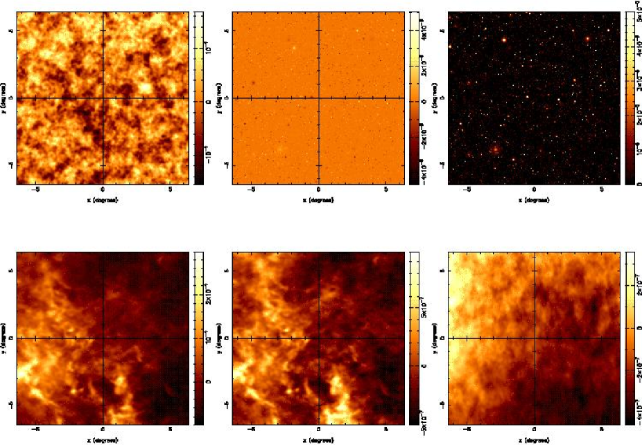
Figure 1: Components present in the simulation at 300 GHz. From left to right and from top to bottom the components are: CMB, kinetic SZ, thermal SZ, Galactic dust, free-free and synchrotron. The spinning dust component has the same spatial template as Galactic thermal dust emission. The units of the maps are $\Delta T/T$.

The Galactic emission is assumed to originate from four different components: thermal dust, spinning dust, free-free and synchrotron. Thermal dust was simulated using the template given by Finkbeiner et al. (1999). This model assumes that dust emission is due to two grey-bodies: a hot one with a dust temperature $T_{D}^{hot}\simeq 16.2K$ and an emissivity $\alpha^{hot}\simeq 2.70$, and a cold one with $T_{D}^{cold}\simeq 9.4K$ and $\alpha^{cold}\simeq 1.67$. These quantities are mean values.

For the free-free template we used one correlated with the dust emission in the manner proposed by Bouchet et al. (1996). The frequency dependence of the free-free emission is assumed to vary as $I_{\nu}\propto\nu^{-0.16}$, and is normalised to give an rms temperature fluctuation of $6.2\mu K$ at 53 GHZ.

The synchrotron spatial template has been produced using the all sky map of Fosalba & Girardino , which is an extrapolation of the 408 MHz radio map of Haslam et al. (1982), from the original 1 deg resolution to a resolution of 5 arcmin. We further extrapolated the small-scale structure to 1.5 arcmin following a power-law power spectrum with an exponent of $-3$. The frequency dependence is assumed to be $I_{\nu}\propto\nu^{-0.9}$ and is normalized to the Haslam 408 MHz map. We include in our simulations information on the changes of the spectral index as a function of electron density in the Galaxy. This template has been made by combining the Haslam map with the Reich & Reich (1986) map at 1420 MHz and the Jonas et al. (1998) map at 2326 MHz, and can be found in the FTP site refered to above.

We have also taken into account the possible Galactic emission due to spinning grains of dust, proposed by Draine & Lazarian (1998). This component could be important at the lowest frequencies of Planck (30 and 44 GHz) in the outskirts of the Galactic plane.

The extragalactic point source simulations follow the same cosmological model as that assumed for the CMB simulation and corresponds to the model of Toffolati et al. (1998). The thermal SZ effect was made for the same cosmological model. The cluster population was modelled following the Press-Schechter formalism (Press & Schechter 1974) with a Poissonian distribution in $\theta$ and $\phi$. The simulated cluster population fits well all the available X-ray and optical cluster data sets (see Diego et al. 2001a for a discussion). The different components used for the simulation are shown at 300 GHz in figure 1. Figure 2 shows the simulated channels taking into account all the components, as well as the antenna beam effect and the instrumental noise.

The simulation described above is the same used by Diego et al. (2001b). We have chosen this particular simulation in order to compare results with that work under the same conditions.

Figure 2: Simulated Planck channels. Each map corresponds to the same $12.8^{\circ}\times 12.8^{\circ}$ area of the sky at the frequency of the channel. The represented channels are, from left to right and from top to bottom, 30, 30, 44, 70, 100 (LFI), 100 (HFI), 143, 217, 353, 545 and 857 GHz. The units of the maps are $\Delta T/T$.

4 RESULTS AND DISCUSSION

4.1 Testing the methods

Before applying the methods presented in section 2 to the simulations described in section 3, let us illustrate how they work in a simplified case. For the sake of simplicity, the simulations include the same foregrounds and technical features as the simulations described in section 3, except for the fact that the spinning dust component was not included. Spinning dust is the weakest component and its contribution is almost negligible in most Planck channels. The other main difference with the realistic simulations is the thermal SZ effect itself. Instead of the realistic SZ clusters, we simulated 200 clusters of the same size ($r_{c}=0.5$ pixels), and amplitudes uniformly distributed between 0 and the maximum amplitude of the clusters belonging to the realistic simulation. The simulated clusters have the frequency dependence of the thermal SZ effect and the radial profile

$$\tau(x)=N\left(\frac{1}{\sqrt{r^{2}_{c}+x^{2}}}-\frac{1}{\sqrt{r^{2}_{v}+x^{2}}}\right)$$ (36)

where $N=r_{v}r_{c}/(r_{v}+r_{c})$. Here $r_{c}$ denotes the core radius and $r_{v}$ is a ‘cut scale’ that can be interpreted as the virial radius of the cluster. The profile given by (36) is a modified multiquadric profile that behaves as a $\beta$ model for $x<<r_{v}$ and decays quickly for $x>>r_{v}$. In order to simplify the simulations still further, the kinematic SZ effect is not included. In the real case, the contribution of the kinematic SZ effect is expected to be $\sim 30$ times lower than the contribution of the thermal SZ effect, thus justifying our approximation.

Figure 3: Filters used to test the multifilter method. Adaptive filter (solid line) and matched filter (dotted line) are represented in Fourier space for each frequency channel.

The simulated maps were filtered using the four possible combinations of filters and methods presented in this work. The combination method took about 1 minute of processing in a 700 MHz PC. The multifilter method took about 10 minutes of processing on the same computer. Processing times were slightly higher for the case of adaptive filters than in the case of matched filters. To compute the filters and the combinations of the maps the low resolution channels were re-binned to the resolution of the highest resolution channel (1.5 arcmin). Figure 3 shows the filters (in Fourier space) employed in the multifilter method. The adaptive filters are represented by solid lines, whereas matched filters are represented by dotted lines. Filters, specially those used in low frequency channels, are quite complicated and show several peaks at different wave numbers $q$ that correspond to the different scales the filters are trying to identify on the images. Conversely, the filters used after the combination method are rather simple and are shown in figure 4. The differences between matched and adaptive filters in the combination method are small. This indicates that there will be few differences in the results of both filters. In the case of the multifilters the differences are more pronounced, in particular for the 217 GHz channel.

The results from the test can be summarised as follows. The number of detections is higher in the multifilter case. This is not surprising since by definition the multifilter method is more powerful than the combination method. In particular, if one raises the detection threshold, the difference between the two methods increases. As an example, table 2 shows the results of one of the tests. After filtering, the sources were detected by looking for peaks above a $4\sigma$ threshold and then compared with a catalogue of the original simulated clusters. By comparison, in the same simulations, if the detection threshold is raised to $5\sigma$ (this case is not shown in table 2) the matched multifilters produce 90 detections whereas the matched filter in the combination method gives only 78.

A detected peak is considered a spurious detection if the distance to the closest object in the original catalogue is greater than 1.5 pixels. The number of spurious detections is strikingly low in all cases. Nevertheless, the adaptive filter seems to work better than the matched filter (for example, in table 2 the adaptive filter gives 0 spurious detections instead of 1 with the combination method). Of all the components present in the simulations, point sources are the most likely to produce spurious detections due to the similar scale of sources and SZ clusters. However, the frequency dependence of the SZ effect greatly reduces the probability of contamination.

The position of the sources was determined with errors below the pixel size (1.5 arcmin). However, the error in the determination of the amplitude is quite large ($\sim 35\%$). Table 2 shows that this error is due to a systematic bias. To explain this bias let us consider the case of matched filter. The filter normalization is given by integral $a=\int^{\infty}_{0}dqq\tau^{2}/P$, being $\tau$ the source profile in Fourier space and $P$ the power spectrum of the background. However, when we analyse a patch of the sky we do not have information about the power spectrum at all the wave numbers $q$. An image divided into pixels is limited by a minimum value $q_{min}$ and a maximum $q_{max}$. Therefore, the normalization we calculate is $a^{\prime}=\int^{q_{max}}_{q_{min}}dqq\tau^{2}/P$. For the case of images with the same size and pixel scale as our simulations, and a multiquadric profile $\tau$ with $r_{c}=0.5$ pixels, the normalisations can differ by $10\%$ for a background spectral index $\gamma=1$ to $60\%$ for a background spectral index $\gamma=3$. The case for adaptive filters is more complicated but qualitatively similar. This bias is independent of the source flux and can be calibrated using simulations.

Figure 4: Filters used to test the combination method. The adaptive filter (solid line) and the matched filter (dotted line) are represented in Fourier space.

Table 2: Results of the test for 10 frequency channels and clusters of equal size ($r_{c}=0.5$ pixels). The detection was performed over the $4\sigma$ threshold in all cases. The filtering method is listed in the first column. Second column shows the number of true detections found over the $4\sigma$ detection threshold. The third column indicates the number of spurious sources detected in each case. The fourth column lists the mean error in the determination of the position of the detected sources. Column five lists the mean relative bias in the determination of the amplitude, defined as $\bar{b}_{A}=100<(A-A_{0})/A_{0}>$. Column six shows the mean relative error in the determination of the amplitude, defined as $\bar{e}_{A}=100<\mid A-A_{0}\mid/A_{0}>$.

METHOD	number of	number of	mean offset	$\bar{b}_{A}(\%)$	$\bar{e}_{A}$ (%)
	detections	spurious	(pixels)
combination/matched	110	1	0.41	33.3	33.3
combination/adaptive	113	0	0.38	32.5	32.5
multifilter/matched	116	1	0.42	29.8	29.9
multifilter/adaptive	109	1	0.57	34.4	34.5

Figure 5 shows the contribution of each channel to the source amplitude estimation for each method. The channels with larger contribution are the 143 GHz and the 353 GHz. This is not surprising since they are the channels with more SZ contribution. The 100 GHz HFI channel has more contribution than the 100 GHz LFI because of its better signal-to-noise ratio. The combination method puts more emphasis in the 100 GHz and less in the 143 GHz channels than the multifilter method. Contributions from the 30 GHz, 217 GHz and 857 GHz channels are negligible. However, that does not mean that these channels do not contribute to the filter construction. For example, if we repeat the analysis with only the 5 channels with more contribution (70, 100 LFI, 100 HFI, 143 and 353 GHz), the number of detections reduces by $\sim 10\%$ and the number of spurious detections increases to 6 (at $4\sigma$ detection threshold) for the combination method case (for the two filters) and to 9 (adaptive filter) and 5 (matched filter) for the multifilter method. Even the 217 GHz channel is important; repeating the analysis with all channels except for the 217 GHz increases the error in the determination of the amplitudes and also increases the number of spurious detections at low $\sigma$ thresholds.

Figure 5: Contributions of the different channels to the source amplitude estimation. The contributions are normalised so that the channel with maximum contribution has contribution 1. Panels corresponding to the combination (matched) and combination (adaptive) are the same, since the weights are assigned before filtering. However, they are both shown for comparison purposes.

We can summarise the conclusions of the test as follows:

• Multifilter method is more powerful in the detection and estimation of cluster parameters.

• Combination method is faster than the multifilter method.

• Multifrequency information reduces the number of spurious detections. Therefore, it is not critical to use an adaptive filter to that end. The matched filter allows one to detect more sources.

• Some channels contribute more than others to the analysis, but all of them carry valuable information; the analysis should include all the available data.

4.2 Results for realistic simulations

Taking into account the insights provided by the test presented in the last sub-section, we are now prepared to confront the analysis of realistic simulations. These realistic simulations have been described in section 3. The main difference with respect to the previously performed test is that in the realistic case clusters have different sizes that are not known a priori. Herranz et al. (2001b) proposed a method to accommodate with this problem:

• Choose a trial core radius $r_{c}$ and construct the corresponding filters.

• Convolve the data with the filters, varying the scales $R_{\nu}$ of eq. (3). This is performed by substituting $\tilde{\psi}(q)$ by $\tilde{\psi}(qx)$, where $x=R_{\nu}^{\prime}/R_{\nu}$ is simply a dilation factor.

• In the case of scale-adaptive filters, condition (iii) (see section 2.2.1) implies that, if the assumed value of $r_{c}$ corresponds with the true core radius of the cluster, the coefficients will be maximum when $x=1$. If this is not true, the trial $r_{c}$ is discarded.

• In the case of matched filters, condition (iii) no longer holds. However, a similar criterion can be used: the best performance of the filter will occur when the scale of the filter and the scale of the cluster is the same. Therefore, if the signal-to-noise ratio of the coefficients is not maximum for $x=1$, the assumed radius $r_{c}$ is not the optimal choice. If this condition is verified for more than one value of $r_{c}$, the one with the highest signal-to-noise ratio is chosen.

• We repeat the process with as many different values of $r_{c}$ as desired.

In Herranz et al. (2001b), the above method has been successfully applied to single frequency maps containing simulated multiquadric profiles and different kind of backgrounds.

The clusters in the realistic simulations have a profile

$$\tau(r)=\frac{2}{\sqrt{1+(r/r_{c})^{2}}}\tan^{-1}\left[\sqrt{\frac{p^{2}-(r/r_{c})^{2}}{1+(r/r_{c})^{2}}}\right],$$ (37)

where $p=r_{v}/r_{c}$ is the ratio between the virial radius and the core radius of the cluster. This profile is realistic from the point of view of the physics of the Sunyaev-Zel’dovich effect. The profiles (36) and (37) are almost identical for $r<r_{v}$. In order to calculate the filters in Fourier space, it is easier to work with the modified multiquadric (36). Therefore, as a first approximation we will assume that the clusters can be described by the profile (36). As we will see, this is a good approximation.

Following the results of the test in the last subsection, we choose a matched multifilter to perform the analysis. After applying our method to the simulations we detect the clusters by looking for sets of connected pixels above a certain threshold. The maximum of these sets give the position and the amplitude of the sources. At the $3\sigma$ level (regions with 5 or more connected pixels) we are able to detect 63 cluster candidates, of which 62 correspond to real clusters. The spurious detection appears in one of the borders of the image and therefore can be considered as an edge effect. The mean error in the determination of the position of the clusters was $\sim 1$ pixel.

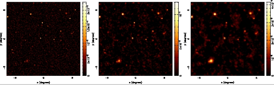
Figure 6: Multifiltered data at several scales. Left panel shows the output after filtering with a matched multifilter that considers that clusters are point-like. Center panel shows the output after filtering with a matched multifilter for a modified multiquadric profile with $r_{c}=1.0$ pixel. Right panel shows the output after filtering with a matched multifilter for a modified multiquadric profile with $r_{c}=2.5$ pixel. Note how different structures are enhanced at different scales. The units of the maps are $\Delta T/T$.

Using the multi-scale analysis we are able to determine the core radii of the clusters with a mean absolute error of 0.30 pixels. The mean bias in the determination of the core radii was $-0.15$ pixels. Since pixelisation effects are expected to corrupt structures whose typical scale is much smaller than the pixel size, all clusters with correspondingly small core radii will not follow the multi-quadric profile. Most of the clusters have very small core radii and therefore can be considered as point-like sources. To detect these clusters, a Gaussian profile (corresponding to the beam at each channel) was assumed instead of the multiquadric given by (36). The separation between clusters that are considered as point sources and extended sources was set in $r_{c}=0.4$ pixel, since if $r_{c}$ is below this limit the FWHM of the multiquadric profile is of the order of a pixel. All the clusters that were detected as point sources were considered to have the (arbitrary) value $r_{c}=0.1$ pixel. The bias in the determination of the core radius mentioned above is due to the asymmetry introduced when assigning $r_{c}=0.1$ pixel to all clusters whose core radius is less than 0.4 pixel. Figure 6 shows the resulting maps after filtering with different scales (point source in the left, $r_{c}=1.0$ pixel in the middle and $r_{c}=2.5$ pixel in the right side). Small clusters stand out mainly in the left panel, while large clusters are emphasized in the right panel.

Figure 7: Amplitudes of the 60 brightest detected clusters vs. true amplitudes. The dotted line corresponds to the perfect situation True Amplitude = Detected Amplitude.

Figure 7 shows the detected amplitudes of the 60 brightest detected clusters vs. the true amplitudes. The brightest sources in the graph were recovered with relative errors of $\sim 30\%$. As might be expected, the error increases as the true amplitude decreases. For the weakest clusters, the detected amplitude tends to a horizontal line. This bias is due to the incorrect determination of the normalization described in section 4.1, as well as two additional factors: first, only the faint clusters that are overamplified are able to reach the detection threshold; second, the detection is performed by looking for peaks in the data and, hence, those clusters which are by chance enhanced by residual fluctuations of the background (noise) are more likely to be detected. The bias due to the normalization should be the same for all sources with a given scale and therefore could be calibrated from simulations, whereas the second kind of bias affects mainly the weak clusters (that dominate the number counts in this case) and can not be easily calibrated. However, the amplitude estimation could be improved by refining the detection method.

The catalogue of detected sources was complete above 0.17 Jy (at 300 GHz). Below this limit the completeness gradually decreases. There are a few very faint clusters that are detected with this method (fluxes of few tens of mJy), but the practical detection limit is $40-50$ mJy (at 300 GHz). The 62 detections in our small sky patch of $(12.8^{\circ})^{2}$ corresponds to $\approx 10000$ detections in $2/3$ of the sky (the area not dominated by the Galaxy).

The performance of the other filtering techniques proposed in this work was compared to the performance of the matched multifilter for the realistic Planck simulations. For the comparison, only the point-like clusters (that dominate the number counts) were considered. The scale-adaptive multifilter, as seen in section 4.1, performs worse than the matched multifilter because their main advantage, that is the removal of spurious sources, has already been accomplished by the multi-frequency information included in the filters. Since the clusters one is trying to detect are very faint, it is the overall gain which is most important. At $3\sigma$, the scale-adaptive multifilter detects 40 per cent fewer clusters than the matched multifilter. Both matched and scale-adaptive filtering of an optimally combined map are slightly less sensitive than multifilters, producing, in both cases, around 20 per cent fewer detections at $3\sigma$ than with the matched multifilter. In other words, in the case of single filters, matched and scale-adaptive perform very similarly (as was expected from figure 4, where both filters look alike).

The results obtained with the matched multifilter are comparable in number of detections and reliability at the $3\sigma$-threshold to those obtained by Diego et al. (2001b). To perform their method it is necessary first to clean the maps carefully. This cleaning includes point source removal with a MHW technique (Vielva el al. 2001a), dust substraction using the 857 GHz map and CMB substraction in Fourier space up to a certain wavenumber limit using the 217 GHz map. In order to compare results, we performed the same cleaning method and then applied the matched multifilter. At $3\sigma$ detection threshold, we obtained a $7$ per cent more detections than before. At $2\sigma$, we also detected $7$ per cent more clusters and the number of spurious detections decreased by about $12$ per cent. This improvement is small given all the cleaning work that is necessary to obtain it. Moreover, it indicates that the multifilter scheme is powerful and robust enough to deal successfully with contaminants such as point sources, dust and the CMB signal.

5 Conclusions

The filtering techniques described in this work have proven to be useful tools for the detection of discrete objects in multifrequency data, which are known to have a prescribed frequency dependence. The only other assumption about the objects is their spatial template; any other quantities of interest are directly calculated from the data. We have assumed in this work that the sources have circular symmetry, but the method can be extended to deal with asymmetric structures. Future work will take this point into account. We have applied these techniques to the problem posed by the presence of Sunyaev-Zel’dovich effect in multifrequency CMB maps. The best results are obtained with matched multifilters. The detection level of the method is comparable to other single-component separation methods, but the number of assumptions and previous data processing is reduced to a minimum. Owing to the weakness of the signals that we aim to detect, the determination of the amplitude of the clusters is biased; this is the strongest limitation of the method. Therefore, the method should be complemented with a posteriori analysis (for example data fitting) in order to improve the amplitude estimation of weak clusters. Finally, the filters here presented can be used in other fields of Astronomy, such as X-ray observations, and large-scale structure detection.

References

- [] Bouchet, F.R., Gispert, R. & Puget, J.L., 1996 in Drew, E., ed., Proc. AIP Conf. 384, The mm/sub-mm foregrounds and future CMB missions, AIP Press, New York, p. 255.
- [] Bouchet, F.R., Gispert, R., Boulanger, F., Puget, J.L., 1997 in Bouchet F.R., Gispert, R., Guiderdoni, B., Tran Thanh Van, J., eds, Porc. 16th Moriond Astrophysics Meeting, Microwave Anisotropies, Editions Frontiere, Gif-sur Yvette, p. 481.
- [] Cayón, L., Sanz, J.L., Barreiro, R.B., Martínez-González, E., Vielva, P., Toffolatti, L., Silk, J., Diego, J.M., Argüeso, F., 2000, MNRAS, 315, 757.
- [] Diego, J.M., Martínez-González, E., Sanz, J.L., Cayón, L., & Silk, J., 2001a, MNRAS, 325, 1533.
- [] Diego, J.M., Vielva, P., Martínez-González, E., Silk, J. & Sanz, J.L., 2001b, MNRAS submitted, astro-ph/0110587.
- [] Draine, B.T., & Lazarian, A., 1998, ApJ, 494, L19.
- [] Finkbeiner, D.P., Davis, M. & Schlegel, D.J., 1999, ApJ, 524, 867.
- [] Haslam, C.G.T., Salter, C.J., Stoffel, H. & Wilson, W.E., 1982, A&AS, 47, 1.
- [] Herranz, D., Gallegos, J., Sanz, J.L., Martínez-González, E., 2001a, MNRAS accepted for publication.
- [] Herranz, D., Sanz, J.L., Barreiro, R.B., Martínez-González, E., 2001b, submitted to ApJ.
- [] Hobson, M.P., Jones, A.W., Lasenby, A.N., Bouchet, F.R., 1998, MNRAS, 300, 1.
- [] Hobson, M.P., Barreiro, R.B., Toffolatti, L., Lasenby, A.N., Sanz, J.L., Jones, A.W., Bouchet, F.R., 1999, MNRAS, 306, 232.
- [] Jonas, J.L., Baart, E.E. & Nicolson, G.D., 1998, MNRAS, 297, 977.
- [] Maino, D., Farusi, A., Baccigalupi, C., Perrota, F., Banday, A.J., Bedini, L., Burigana, C., De Zotti, G., Górsky, K.M. & Salerno, E., 2001, MNRAS submitted, astro-ph/0108362.
- [] Naselsky, P., Novikov, D. & Silk, J., preprint (astro-ph/0111168)
- [] Press W.H. & Schechter, P., 1974, ApJ, 187, 425.
- [] Sanz, J.L., Herranz, D. & Martínez-González, E., 2001, ApJ, 552, 484.
- [] Seljak, U., & Zaldarriaga, M., 1996, ApJ, 469, 437.
- [] Tegmark, M. & Efstathiou, G., 1996, MNRAS, 281, 1297.
- [] Tegmark, M. & de Oliveira-Costa, A., 1998, MNRAS, 500, 83.
- [] Toffolatti, L., Argüeso, F., De Zotti, G., Mazzei, P., Franceschini, A., Danese, L. & Burigana, C., 1998, MNRAS, 326, 181.
- [] Vielva, P., Martínez-González, E., Cayón, L., Diego, J.M., Sanz, J.L. & Toffolatti, L., 2001a, MNRAS, 326, 181.
- [] Vielva, P., Barreiro, R.B., Hobson, M.P., Martínez-González, E., Lasenby, A.N., Sanz, J.L. & Toffolatti, L., 2001b, MNRAS, 328, 1.