THE CRAB NEBULA: INTERPRETATION OF CHANDRA OBSERVATIONS

Abstract

We interpret the observed X-ray morphology of the central part of the Crab Nebula (torus $+$ jets) in terms of the standard theory by Kennel and Coroniti (1984). The only new element is the inclusion of anisotropy in the energy flux from the pulsar in the theory. In the standard theory of relativistic winds, the Lorentz factor of the particles in front of the shock that terminates the pulsar relativistic wind depends on the polar angle as $\gamma=\gamma_{0}+\gamma_{m}\sin^{2}\theta$, where $\gamma_{0}\sim 200$ and $\gamma_{m}\sim 4.5\times 10^{6}$. The plasma flow in the wind is isotropic. After the passage of the pulsar wind through the shock, the flow becomes subsonic with a roughly constant (over the plerion volume) pressure $P={1\over 3}n\epsilon$, where $n$ is the plasma particle density and $\epsilon$ is the mean particle energy. Since $\epsilon\sim\gamma mc^{2}$, a low-density region filled with the most energetic electrons is formed near the equator. A bright torus of synchrotron radiation develops here. Jet-like regions are formed along the pulsar rotation axis, where the particle density is almost four orders of magnitude higher than that in the equatorial plane, because the particle energy there is four orders of magnitude lower. The energy of these particles is too low to produce detectable synchrotron radiation. However, these quasi-jets become comparable in brightness to the torus if additional particle acceleration takes place in the plerion. We also present the results of our study of the hydrodynamic interaction between an anisotropic wind and the interstellar medium. We compare the calculated and observed distributions of the volume intensity of X-ray radiation.

Key words: plasma astrophysics, hydrodynamics and shock waves.

INTRODUCTION

The Crab Nebula is one of the most interesting and best-studied sources in the sky. This object was observed over a wide wavelength range: from radio to gamma-rays with a photon energy of 50 TeV (Aharonian 2000; Hester 1998; Shklovskii 1968). However, advances in observational astronomy provide new data on the Crab Nebula. In the last decade, progress in the technology of X-ray telescopes has allowed the Crab Nebula to be observed with an angular resolution comparable to the angular resolution of ground-based optical telescopes. As would be expected, this gave completely new information on the structure of the central part of the nebula. The data obtained on the Chandra X-ray observatory arouse particular interest.

The Chandra observations show that the central part of the nebula consists of two components in the soft X-ray emission: a toroidal structure surrounding the pulsar PSR $0531+21$ and two jet-like features located perpendicular to the torus and emerging from the pulsar (Weisskopf et al. 2000). Interestingly, such a structure of the plerion central region is also observed in the Vela pulsar (Pavlov et al. 2001) and in the supernova remnant G$0.9+1$ (Gaensler 2001). In this paper, we focus our attention on the Crab Nebula primarily because of the parameters of the relativistic plasma flow (pulsar wind) from this pulsar. Weak magnetation of the wind from PSR $0531+21$ allows the problem of its interaction with the interstellar medium to be simplified to an extent that the intensity y distribution of synchrotron radiation in the plerion can be easily estimated and compared with the observed one.

The first impression that arises when studying the Chandra images of the Crab Nebula is that the toroidal structure surrounding the pulsar suggests the presence of an accretion disk around the nebula. However, this interpretation of the observed picture is incorrect for obvious reasons. First, there is no independent evidence for the existence of a second companion and an accretion disk around the Crab pulsar. Second, the characteristic size of the toroidal structure itself, $\sim 10^{18}$ cm, rules out the possibility of the disk interpretation of the observed picture.

The situation with the jet-like features is more complicated. Jets are observed from many Galactic YSO (Livio 1999), SS 433 (Cherepashchuk 1998), superluminal sources (Mirabel and Rodrigues 1998) and AGN (Urri and Padovani 1995). A direct analogy between the jets from these objects and those observed in the Crab Nebula suggests itself. The assumption that the pulsar itself ejects collimated plasma flows seems reasonable enough. However, it is most likely incorrect.

The Crab Nebula is a typical plerion — a bubble of relativistic particles frozen in a magnetic field. This bubble is formed when the flow of supersonic relativistic plasma (pulsar wind) ejected by the pulsar interacts with the interstellar medium. Since the wind itself is cold, it remains unobservable thus far (see, however, Bogovalov and Aharonian 2000). After passing through the wind-terminating shock, the particles are isotropized and begin to emit synchrotron photons over a wide electromagnetic spectral range, producing the observed plerion radiation; hence the fundamental difference between the jet-like features observed in the nebula and the actual jet flows observed in the Universe from other objects. The latter are the supersonic collimated flows ejected from the source. They are characterized by termination when interacting with the interstellar medium to produce a shock and the so-called lobes (Ferrari et al. 1996). The jet-like features themselves in the Crab Nebula are formed behind the shock that terminates the pulsar wind. The plasma flow in them is definitely subsonic. Therefore, the physics of this phenomenon undoubtedly differs from the physics of the processes that give rise to astrophysical jets.

Since the observed structures in the Crab Nebula result from the interaction of the pulsar wind with the ambient medium, the pattern of this interaction must be studied to understand their nature. The interaction of the wind from the Crab pulsar with the interstellar medium has been analyzed by many authors. Rees and Gunn (1974) and Kennel and Coroniti (1984) first gave important constraints on the parameters of the pulsar wind immediately in front of the shock. The calculated plerion expansion velocity, luminosity, and synchrotron radiation spectrum (from optical wavelengths to X-rays) agree with the observed ones if the wind consists of electrons and positrons with a Lorentz factor of $\sim 3\times 10^{6}$ and if almost all of the pulsar rotational losses are transformed into the particle kinetic energy so that the ratio of the electromagnetic energy flux to the particle kinetic energy flux is $\sigma=3\times 10^{-3}$. For such wind parameters, we can also naturally explain the gamma-ray emission from the Crab Nebula above 10 GeV, which is generated by the inverse Compton scattering of the same electrons that generate the synchrotron radiation (Atoyan and Aharonian 1996; de Jager and Harding 1992).

The success of the theory by Kennel and Coroniti (1984) was achieved through a significant simplification of the problem. This theory assumes the problem to be spherically symmetric. As long as the analysis was restricted to the integrated characteristics of the radiation from the Crab Nebula (spectra, luminosity), this limitation was not fundamental in nature. However, the observed X-ray morphology of the Crab Nebula cannot be explained in terms of this theory. Clearly, the Crab Nebula is not spherically symmetric. The more realistic pattern of interaction between an anisotropic pulsar wind and the interstellar medium must be considered. Here, we made the first step in solving this problem. At this stage, we do not set the goal of developing a full-blown theory of the interaction between an anisotropic, magnetized pulsar wind and a homogeneous interstellar medium. This is not yet possible. Here, we determine the pattern of pulsar-wind anisotropy by using the results that have been obtained in pulsar physics in recent years. We also perform a semiquantitative analysis of the result of the interaction between such a wind and the interstellar medium, including an estimation of the synchrotron radiation. In the end, we wish to understand whether the level of anisotropy in pulsar winds that follows from the pulsar theory is enough to explain, at least in general terms, the structure of the central part of the Crab Nebula observed on the Chandra observatory.

THE PULSAR WIND FROM PSR 0531 + 21

The integrated characteristics of the Crab Nebula can be naturally explained in terms of the theory by Kennel and Coroniti (1984) if the wind magnetization parameter is $\sigma=3\times 10^{-3}$ and the wind Lorenz factor is $\gamma\sim 3\times 10^{6}$ immediately in front of the shock (Kennel and Coroniti 1984), although other wind parameters cannot be completely ruled out either (Begelman 1998). The Kennel–Coroniti theory naturally accounts for the source spectrum over an unprecedentedly wide wavelength range, from optical to hard gamma-ray emission (fifteen orders of magnitude in wavelength!). No theory in astrophysics can boast a similar success. However, there is one problem in this theory that spoils the overall picture. It is not yet clear how the pulsar PSR $0531+21$ produces the relativistic wind with such parameters. This remains one of the key puzzles in the physics of radio pulsars.

The problem is that all the currently available theories of particle acceleration and plasma formation in pulsar magnetospheres [the polar-cap theory (Arons 1983; Daugherty and Harding 1996) or the outer-gap theory (Romani 1996; Cheng et al. 2000)] are capable of explaining how the dense $e^{\pm}$ plasma that produces a relativistic particle wind is formed. However, this plasma carries a negligible fraction ($\sim 10^{-4}$) of all rotational losses from the Crab pulsar. The entire energy flux from the pulsar is concentrated in the electromagnetic field carried away by the wind, which corresponds to the wind magnetization parameter $\sigma\sim 10^{4}$. The wind itself has a modest Lorentz factor $\sim 200$ near the radio-pulsar light cylinder (Daugherty and Harding 1996). It is yet tbe clarified through which processes almost the entire electromagnetic energy flux is transformed into the wind-particle kinetic energy on the way from the light cylinder to the shock front, although substantial efforts were spared to solve this problem (Coroniti 1990; Lyubarsky and Kirk 2001).

There is no need to know the wind acceleration mechanism to determine the energy-fl mux distribution in the wind. The fact that the conservation of the energy flux in the wind holds in any case is suffice. The point is that the electromagnetic energy flux in the winds from radio pulsars propagates along streamlines. The plasma kinetic energy flux also propagates along these streamlines. This conclusion is based on MHD models of the winds from axisymmetrically rotating objects (Okamoto 1978). However, it has recently been shown to be also valid for obliquely rotating objects where the flow beyond the light cylinder is concerned (Bogovalov 1999). This ensures that the total energy flux per particle is conserved along a given streamline. The kinetic energy flux per particle, in units of $mc^{2}$, is $\gamma$. The electromagnetic energy flux per particle, in units of $mc^{2}$, is

$$s={c\over 4\pi}[E\times B]/(nvmc^{2}\gamma),$$ (1)

where $E$ is the electric field, $B$ is the magnetic field, $n$ is the particle density in the intrinsic frame of reference, and $v$ is the wind velocity. The sum $\gamma+s$ depends on the streamline but is conserved along it. It follows from the solution of the problem on the structure of the wind from an oblique rotator (Bogovalov 1999) that the energy flux in the wind sufficiently far from the light cylinder may be considered to be azimuthally symmetric, although the electromagnetic field itself is not azimuthally symmetric in this case (see Bogovalov (1999) for details). In this notation, the magnetization parameter is $\sigma=s/\gamma$. The conservation of the total energy flux ensures that

$$\gamma_{0}+s_{0}=\gamma+s.$$ (2)

The subscript ‘0’ marks the values near the light cylinder. Since $s\ll\gamma$ in front of the shock that terminates the pulsar wind, the Lorentz factor of the preshock plasma may be assumed to be $\gamma=\gamma_{0}+s_{0}$. Thus, the dependence of the particle energy on the streamline along which the particles move is determined by their initial energy and the initial distribution of the electromagnetic energy flux. We make the only assumption. Assume that the initial distribution of the electromagnetic energy flux does not depend on (or is almost independent of) the wind acceleration. This assumption holds true in all cases if the wind is accelerated sufficiently far from the light cylinder in the supersonic flow region. Then, the field distribution in the magnetosphere and, hence, the initial electromagnetic energy flux do not depend on what happens downstream of the magnetosonic surface. This is because no MHD signal can penetrate from the supersonic flow region into the subsonic flow region and affect the flow in this region. If this is the case, then it will suffice to determine $s_{0}$, provided that there is no acceleration.

Numerical and analytical calculations of the relativistic plasma flow show that the plasma magnetic collimation is negligible for Lorentz factors $\gamma>200$ (Beskin 1998; Bogovalov and Tsinganos 1999; Bogovalov 2001). The pulsar wind may be assumed to spread out radially. Since the relation $E={r\sin\theta\Omega\over c}B_{p}$ (Mestel 1968), where $r$ is the distance to the pulsar, $\theta$ is the polar angle, $\Omega$ is the pulsar angular velocity, and $B_{p}$ is the poloidal magnetic field in the wind, holds between the electric field in the wind and the poloidal magnetic field, the condition for the magnetic field being frozen in the plasma $E+{1\over c}[E\times B]=0$ takes the form

$$r\sin\theta\Omega B_{p}+B_{\varphi}v_{p}=v_{\varphi}B_{p}.$$ (3)

At $r\gg c/\Omega$, the plasma angular velocity tends to zero, because the angular momentum of the plasma particles ($r\sin(\theta)v_{\varphi}$) is limited above. We then derive a simple expression for the toroidal field in the wind far from the pulsar, $B_{\varphi}={r\sin\theta\Omega\over v_{p}}B_{p}$. Therefore, the electromagnetic energy flux per particle (in units $mc^{2}$) is

$$s_{0}=\sin^{2}\theta\left({\Omega r\over v_{p}}\right)^{2}{B_{p}^{2}\over 4\pi n_{0}mc^{2}\gamma_{0}}.$$ (4)

We see that when the relativistic wind spreads out radially and uniformly, the Lorentz factor $\gamma_{1}$ of the preshock wind particles must have a latitude dependence of the form

$$\gamma_{1}=\gamma_{0}+\gamma_{m}\sin^{2}\theta,$$ (5)

where $\gamma_{m}=({\Omega r\over v_{p}})^{2}{B_{p}^{2}\over 4\pi n_{0}mc^{2}\gamma_{0}}$. This is the maximum Lorentz factor of the preshock wind particles. To be consistent with the theory by Kennel and Coroniti (1984), it must be of the order of $3\times 10^{6}$.

Note that expression (5) for the particle Lorentz factor immediately follows from the MHD theory of magnetized winds from rotating objects and is almost model-independent. It only assumes that the particle flux from the pulsar is isotropic. Clearly, this assumption does not severely restrict the range of applicability of our results. For the standard parameters $\gamma_{0}=200$ and $\gamma_{m}\sim 3\times 10^{6}$, the Lorentz factor changes with latitude by four orders of magnitude. Even if the particle flux changes with latitude by several times (or several tens of times), this does not change the overall dependence. Anyway, the most energetic particles will be near the equator and their Lorentz factor will be higher than the Lorentz factor of the particles at the rotation axis by several orders of magnitude.

Below, for our calculations, we assume the wind flow to be radial with an isotropic mass flux. The plasma density in the intrinsic frame of reference in such a wind is

$$n_{1}={\dot{N}\over 4\pi v_{p}r^{2}\gamma}.$$ (6)

Here, $\dot{N}$ is the rate of particle injection into the nebula. The toroidal magnetic field has the distribution

$$B_{\varphi}={B_{0}r_{0}\sin\theta\over r},$$ (7)

The quantity $B_{0}$ can be determined from the condition $\sigma=3\times 10^{-3}$. We ignore the poloidal magnetic field, because it is much weaker than the toroidal magnetic field ahead of the shock front. The plasma Lorentz factor is given by expression (5). Our objective is to determine (at least qualitatively) how a wind with the above parameters interacts with a homogeneous ambient interstellar medium.

THE APPROXIMATIONS

The problem of the interaction between a highly anisotropic, magnetized relativistic wind and a homogeneous ambient medium has no analytic solution. Even obtaining a numerical solution seems problematic so far. Below, we make two reasonable simplifications that will allow us to answer the questions of interest by using simple mathematics.

(1) The approximation of a hydrodynamic interaction. In the special case of the Crab Nebula, as a first approximation, we may disregard the magnetic-field effect on the postshock plasma dynamics. This approximation seems reasonable, because the pulsar wind from PSR $0531+21$ is weakly magnetized. Recall that the ratio of the preshock Poynting flux to the plasma kinetic energy flux is $\sigma=3\times 10^{-3}$. Although the magnetic field increases in strength by a factor of 3 after the shock passage, the ratio of magnetic pressure to plasma pressure is small up to distances approximately equal to five shock radii (see Kennel and Coroniti 1984). Further out, the magnetic pressure is higher than the plasma pressure and it cannot be ignored. However, the region of $5r_{\mathrm{sh}}$ completely suits us. It is in this region that the most interesting features of the central part of the Crab Nebula are formed: the X-ray torus and the jet-like features. Therefore, below, the wind interaction is considered as a purely hydrodynamic one. We will determine the magnetic-field evolution from the induction equation with a given distribution of the plasma velocity field. Note that although the magnetic-field effect on the plasma dynamics immediately behind the shock wave is marginal, Lyubarsky (2002) attempts to explain the observed jets in the Crab Nebula as resulting from a magnetic compression of the wind after the shock wave. Below, we show that these jets are formed in the hydrodynamic approximation without any involvement of the magnetic field.

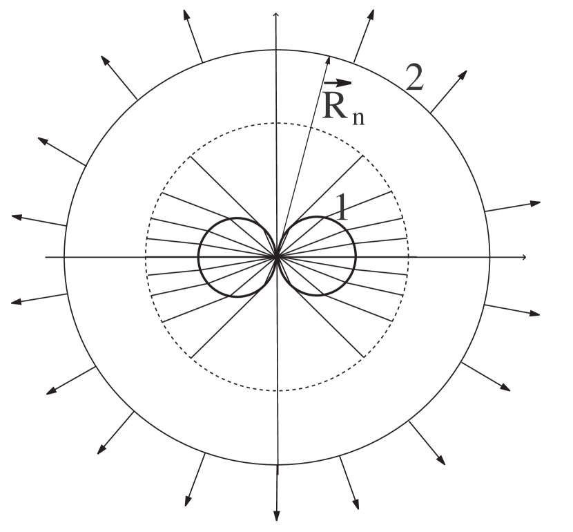
Figure 1: A schematic image of the interaction between the pulsar wind and the interstellar medium. Because of the increase in the energy flux density in the wind toward the equator, the shock (1) takes the form of a torus. The streamlines bend at the shock front and are pressed to the equator. The region between the shock and the contact discontinuity (2) is filled with relativistic particles emitting synchrotron radiation. The dotted line marks the $r\ll R_{n}$ region, where the plasma flow may be considered to be quasi-steady

(2) The quasi-stationary approximation. Strictly speaking, the interaction of a supersonic wind from the central source with the interstellar medium is not stationary. It is schematically shown in Fig. 1. The source continuously injects new particles into the nebula and the nebula size increases with time. However, in a bounded region of space near the shock, the flow may be considered to be steady, provided that the nebula size is much larger than the characteristic size of the shock. This is easy to understand from simple considerations. Assume that the source injects particles with characteristic energy $\epsilon$ into the nebula at a rate $\dot{N}$. The nebula size $R_{n}$ at constant external pressure $P_{\mathrm{ext}}$ is then determined by the relation $\dot{N}t\epsilon/(4\pi/3R_{n}^{3})=p_{\mathrm{ext}}$, where $t$ is the source operation time. We see from this relation that the nebula radius increases as $t^{1/3}$. This means that the velocity of the nebula outer rim decreases with time; therefore, the entire flow may be considered in the limit $t\rightarrow\infty$ as steady with the boundary condition at infinity $v\rightarrow 0$ for $r\rightarrow\infty$ and $P=P_{\mathrm{ext}}$. Thus, the condition for applicability of the quasi-stationary approximation is $R_{n}\gg r_{\mathrm{sh}}$, where $r_{\mathrm{sh}}$ is the characteristic radius of the shock front. For the Crab Nebula, $R_{n}\approx 2$ pc and the shock radius is $r_{\mathrm{sh}}=0.1$ pc (Kennel and Coroniti 1984). Consequently, the postshock flow for the Crab Nebula within $5r_{\mathrm{sh}}$ may actually be considered to be steady.

THE INTERACTION OF A HIGHLY ANISOTROPIC WIND WITH THE INTERSTELLAR MEDIUM

Basic Simplifications

The problem of the interaction between a supersonic, highly anisotropic plasma flow and a homogeneous medium has no exact solution so far. Therefore, below, to estimate the observed effects that must arise during such an interaction, we proceed as follows: first, we use a highly simplified interaction model to calculate the volume luminosity of the plerion produced by a Crab-type pulsar; subsequently, we qualitatively consider how our simplifications affect the results of our calculations by using, in particular, the results obtained for weak anisotropy in Appendix A.

We use the following simplifications to estimate the volume luminosity of the Crab Nebula:

(1) Since the postshock plasma flow is subsonic, with the plasma velocity tending to zero when moving downstream of the shock, the plasma density along a streamline may be assumed to be constant (Landau and Lifshitz 1986). The subsonic motion also implies an approximate equality of the pressure in the plerion. Previously, Begelman (1992) used this approximation to describe the postshock flow. Let us estimate the accuracy with which these conditions may be considered to be satisfied in our specific case. The pressure variation in the plerion is $\Delta P/P\sim Wu^{2}/P$. Here, $W=4P$ and $u\sim 1/\sqrt{8}$, because the plasma velocity is $v={1\over 3}c$ immediately behind the shock and then rapidly decreases. Therefore, in the worst case, we have $\Delta P/P\sim 0.5$. This error completely suits us, because below, we are concerned with the variations in mean particle energy $\epsilon$ and plasma density $n$ across a streamline, which are four orders of magnitude; the pressure is related to these quantities by $P={1\over 3}n\epsilon$. Against the background of such variations, the pressure variations of $50\%$ are of no fundamental importance.

(2) We assume the postshock streamlines to remain radial without bending at the shock and use the conditions for a perpendicular shock to determine the postshock plasma parameters.

The Shape of the Shock Front

To determine the shape of the shock front, we use the shock-adiabat relation (A.18) for an oblique shock wave. After the passage of the shock front, the plasma on each streamline adiabatically decelerates; far from the shock front, its velocity tends to zero and the plasma pressure comes into equilibrium with the external pressure $P_{\mathrm{ext}}$. The relationship between the plasma parameters immediately after the shock and $P_{\mathrm{ext}}$ is given by the Bernoulli equation for a relativistic plasma

$$4\gamma_{2}{P_{2}\over n_{2}}=4{P_{\mathrm{ext}}\over n_{\infty}}=\gamma_{1}mc^{2}.$$ (8)

Here, we use the constancy of the Bernoulli integral at the shock front and the relativistic-plasma approximation $e=3p$, which holds good behind the shock. Below, the subscripts ‘1’ and ‘2’ denote the preshock and postshock quantities, respectively.

It is easy to find from these relations and from the adiabatic flow condition (A.5) that

$${P_{\mathrm{ext}}\over\gamma_{1}^{2}n_{1}mc^{2}}={3\over 2}\left({3\over\sqrt{8}}\right)^{{\delta\over\delta-1}}\gamma_{||}^{{2-\delta\over\delta-1}}.$$ (9)

The location of the shock front could be determined from this equation if $\gamma_{||}$ were known. Since the problem is azimuthally symmetric, this quantity is known only at points on the equatorial plane and on the rotation axis. The shock front crosses them at a right angle. Below, we consider a simplified case by assuming, for simplicity, that $\gamma_{||}=1$ everywhere. We then obtain for the shock radius

$$r_{\mathrm{sh}}=\sqrt{{3\over 2}\left({3\over\sqrt{8}}\right)^{{\delta\over\delta-1}}{\gamma_{1}mc^{2}\dot{N}\over 4\pi P_{\mathrm{ext}}c}}.$$ (10)

In the limit $\gamma_{m}\gg\gamma_{0}$ of interest, the shock radius may be assumed to be $r_{\mathrm{sh}}=r_{\mathrm{eq}}|\sin\theta|$ everywhere, except for a narrow interval of angles $\theta<\sqrt{\gamma_{0}/\gamma_{m}}$. This implies that the shock front is generally a torus whose cross section is a couple of contacting circumferences with the centers on the equatorial plane in the middle of the distance $r_{\mathrm{eq}}$ from the source to the shock.

To estimate an error in using everywhere the approximation $\gamma_{||}=1$, we must solve the problem more accurately. Our analysis, which is beyond the scope of this paper, shows that the shock front lies at slightly larger distances than (10). In addition, a system of two shocks is formed near the axis for a highly anisotropic wind. Nevertheless, expression (10) gives an error in the shock radius within $15\%$. In this paper, such an accuracy is admissible.

The Formation of a Toroidal Structure

As follows from the condition of a constant density along the postshock streamline, the plasma velocity $v_{p}$ on each streamline behaves as

$$v_{p}={1\over 3}c\left({r_{\mathrm{sh}}(\theta)\over r}\right)^{2},$$ (11)

where $r_{\mathrm{sh}}(\theta)$ is the distance from the pulsar to the shock location at a given angle $\theta$. This dependence on $r$ follows from the conservation of mass flux for radial plasma motion.

On a given streamline, the dependence of the magnetic field on $r$ and $\theta$ follows from the frozen-in condition. According to this condition, $B/nr=\mathrm{const}$ on a streamline (Landau and Lifshitz 1982). For the preshock magnetic field, we use the condition

$${(B_{0}{r_{0}\over r_{\mathrm{sh}}}\sin\theta)^{2}\over 4\pi n_{1}mc^{2}\gamma_{1}^{2}}=\sigma{\gamma_{m}\sin^{2}\theta\over\gamma_{1}}.$$ (12)

It implies that the ratio of the Poynting flux density to the plasma kinetic energy flux density is everywhere equal to the same value $\sigma$, except for a narrow region near the rotation axis where the toroidal field must vanish. We inserted the additional factor ${\gamma_{m}\sin^{2}\theta\over\gamma}$ in the right-hand part of Eq. (12) to take into account this circumstance. It follows from expression (9) that the preshock magnetic field is

$$B_{1}=B_{0}{r_{0}\over r_{\mathrm{sh}}}\sin\theta=\sqrt{4\sigma\pi\gamma_{m}\gamma_{1}n_{1}mc^{2}}\sin\theta.$$ (13)

Given that the magnetic field increases in strength by a factor of 3 after the passage of a strong shock, we obtain

$$B_{2}=3\sqrt{({4\pi\sigma\gamma_{m}\over\gamma}{2\over 3}\left({\sqrt{8}\over 3}\right)^{{\delta\over\delta-1}}P_{\mathrm{ext}})}\sin\theta{r\over r_{\mathrm{sh}}}.$$ (14)

At angles $\theta\gg\sqrt{\gamma_{0}/\gamma_{m}}$, the expression for the magnetic field takes the form

$$B_{2}=B_{\mathrm{eq}}{r\over r_{\mathrm{sh}}},$$ (15)

where $B_{\mathrm{eq}}$ is the postshock equatorial magnetic field. We see that the field immediately behind the shock is everywhere the same, except for a narrow region near the rotation axis. Outside this region, the field more rapidly increases with distance from the pulsar at high latitudes. The field linearly increases until the magnetic energy density becomes equal to the plasma energy density. Subsequently, the field begins to decrease with increasing $r$ (Kennel and Coroniti 1984). The fact that the linear dependence extends to $5r_{\mathrm{sh}}$ (Kennel and Coroniti 1984), within which the toroidal structure is formed, will suffice.

To calculate the synchrotron radiation, we assume, as in Kennel and Coroniti (1984), that the following power-law particle spectrum is formed behind the shock:

$$F(\gamma,r=r_{\mathrm{sh}})=A\left({\gamma\over\gamma_{\min}}\right)^{-\alpha}\eta(\gamma-\gamma_{\min})\eta(\gamma_{\max}-\gamma),$$ (16)

where $A$ is the normalization factor determined from the particle injection rate on a given streamline, $\gamma_{min}$ is the minimum particle energy in the spectrum, $\gamma_{max}$ is the maximum particle energy in the spectrum, and $\eta(x)$ is the step function equal to unity at $x\geq 1$ and zero at $x<1$.

The mean energy of the chaotic particle motion in this spectrum must correspond to the mean postshock particle energy determined from the shock adiabat. It follows from this condition that

$$\gamma_{\min}={\gamma_{1}(\theta)\over\sqrt{2}}{(\alpha-2)\over(\alpha-1)}$$ (17)

Here, we use the fact that although the cutoff energy of the spectrum, $\gamma_{\max}\approx 5\times 10^{9}$ (Atoyan and Aharonian 1996), is finite, it is much larger than $\gamma_{\min}\leq 5\times 10^{5}$.

The plasma moves behind the shock as a whole at velocity (11). The evolution of the particle spectrum during this motion is described by the transport equation

$$v_{p}{\partial F\over\partial r}=-{\partial\over\partial\gamma}{\dot{\gamma}}F$$ (18)

The rate of change in the Lorentz factor of the chaotic particle motion, $\dot{\gamma}$, is generallyly determined by synchrotron losses and plasma heating thrgh adiabatic compression during the wind deceleration. In our case, the adiabatic changes in particle energy can reach $24\%$ of the particle energy. However, we disregard these changes here, because this is a clear excess of the accuracy under our assumptions about the postchosk plasma dynamics.

The solution of Eq. (18), provided that the distribution function at the shock matches function (16), is

$$f(\gamma,r,\theta)={(1-\gamma G)^{(\alpha-2)}(\alpha-1)\over\gamma_{\min}}\left({\gamma\over\gamma_{\min}}\right)^{-\alpha}\times$$ (19)

$$\times\eta\left({\gamma\over 1-\gamma G}-\gamma_{\min}\right)\eta\left(\gamma_{\max}-{\gamma\over(1-\gamma G)}\right)n(r,\theta).$$

In this expression, the function

$$G(r,\theta)={2\over 5}r_{\mathrm{sh}}(\theta)\left({e^{2}\over mc^{2}}\right)^{2}{B_{\mathrm{eq}}^{2}\over mc^{2}}\left(\left({r\over r_{\mathrm{sh}}(\theta)}\right)^{5}-1\right)$$ (20)

describes the degradation of the particle energy through synchrotron losses. The function $n(r,\theta)$ is the emitting-electron density in the observer’s frame of reference. The electron density in the plerion on the streamline with $\theta$ follows from expression (6):

$$n(r,\theta)={3\dot{N}\over 4\pi cr_{\mathrm{sh}}^{2}(\theta)}.$$ (21)

Here, we took into account the fact that the density at the shock increases by a factor of 3. The synchrotron flux is determined by the convolution of spectrum (19) with the spectral distribution of the radiation from an individual electron (Landau and Lifshitz 1973). The input parameters for our calculations are the particle injection rate $\dot{N}=5\times 10^{38}$ part. s^-1, the maximum Lorentz factor of the wind at the equator $\gamma_{m}=4.5\times 10^{6}$, and the shock location at the equator; we correlated the latter with the inner ring of the toroidal structure, which is located at $r_{\mathrm{eq}}=4.3\times 10^{17}$ cm corresponding to a distance of $14^{\prime\prime}$ (Weisskopf et al. 2000). Actually, this implies that the external pressure $P_{\mathrm{ext}}$ was chosen so that the shock at the equator was located on the inner ring of the toroidal structure.

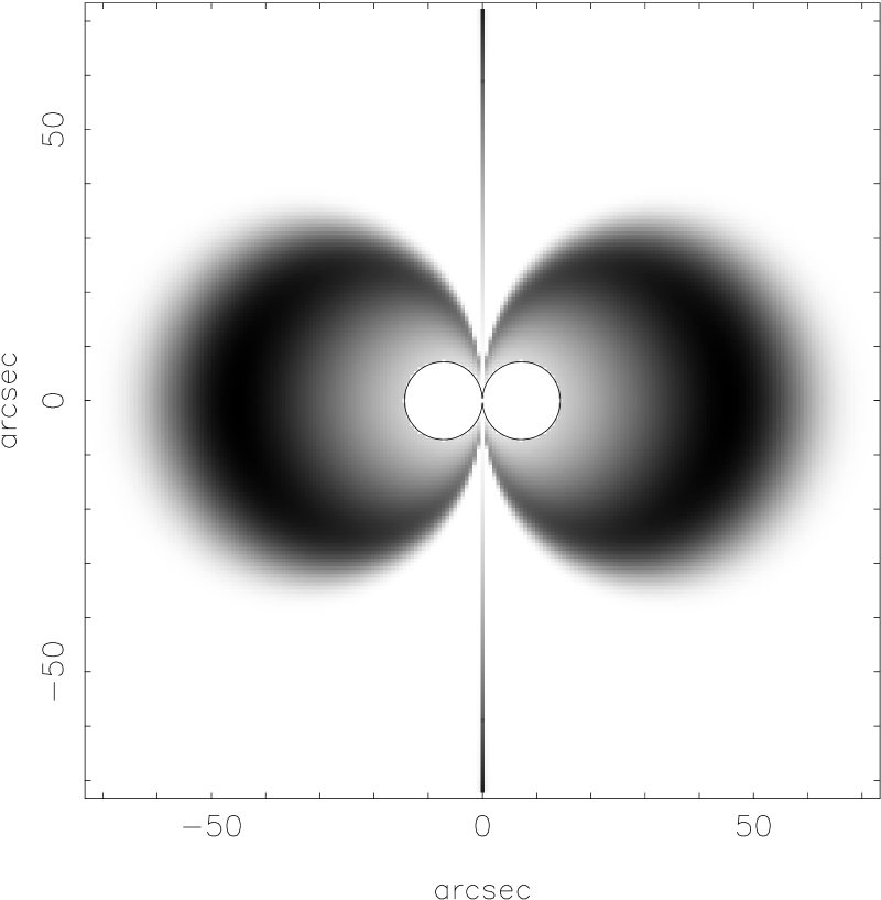
Figure 2: The distribution of the volume emissivity of synchrotron radiation in the plerion produced by the wind from the pulsar PSR $0531+21$. The cross section of the shock is similar in shape to two contacting circumferences. The shock location at the equator is taken to be $14^{\prime\prime}$, in accordance with the observed location of the torus inner ring.

The results of our calculations are presented in Fig. 2. This figure shows the plerion volume luminosity at photon energy 400 eV, the characteristic energy at which the Chandra observations are carried out (Weisskopf et al. 2000). No integration along the line of sight was performed. All geometric sizes were reduced to the pulsar distance, 2 kpc. Here, only the plerion cross section in the poloidal plane is shown. We see that the spatial distribution of the volume luminosity has the shape of a torus with the characteristic sizes corresponding to the observed ones. The radiation reaches the highest intensity at a distance of $\approx 40^{\prime\prime}$, where the second outer ring in the Crab Nebula is located. The intensity of the synchrotron radiation behind the shock is known to gradually rise (Kennel and Coroniti 1984). This rise results from a linear increase in the magnetic field behind the shock, which takes place only if the preshock wind was weakly magnetized. The further rapid decline in the radiation at distances $>60^{\prime\prime}$ is attributable to fast synchrotron electron cooling in the growing magnetic field. We see that although our calculations are definitely incorrect for $r>5R_{\mathrm{sh}}$, this is of no importance. When the electrons reach this region, they have already cooled down to an extent that they do not produce detectable radiation in the Chandra spectral range.

In our calculations, we failed to obtain the bright inner toroidal ring. It may well be that this brightening cannot be explained in terms of magnetic hydrodynamics in principle and that it is attributable to the structure of a collisionless shock, which must be investigates separately (see Gallant 1992).

Across the equatorial plane, the agreement with the observed distribution is slightly worse. The distribution of the calculated brightness across the equator is broader than that of the observed one. It may well be that distributions (5)–(7) do not faithfully describe the preshock wind parameters. The energy and plasma fluxes in the wind may be more concentrated toward the equator than follows from the theory. In our view, however, it is too early to draw this conclusion. The observed disagreement may be entirely attributable to our approximations. We assumed the shock to be perpendicular to the streamline everywhere. This is not true outside the equatorial plane, where the shock inclination to the streamline decreases while $\gamma_{||}$ increases. As the angle of incidence of the shock decreases, the mean energy of the chaotic particle motion after the shock passage also decreases, as is clearly seen from the relation for the shock adiabat of an oblique relativistic shock. Therefore, the volume intensity must decline with height above the equator faster than in our case.

We disregarded the fact that the streamlines must bend toward the equator at the shock, as is the case for weak anisotropy under consideration. Allowing for this circumstance will cause an increase in the brightness near the equator and its faster decrease under it. Finally, we assumed the streamlines after the shock passage to remain straight. In fact, as our calculations for low anisotropy show, the streamlines continue to approach the equator, at least in some preshock region, even after the shock passage. Thus, all our most important approximations used to estimate the volume luminosity of the plerion produced by the Crab pulsar lead to the same effect: a broader distribution of the radiation intensity than must be in the case of a more accurate calculation. Therefore, so far we have no reason to believe that distributions (5)–(7) inaccurately describe the preshock parameters of the wind from the Crab pulsar.

Jet-like Features

In the model that is a simple generalization of the model by Kennel and Coroniti (1984), we failed to obtain something similar to the bright jet-like features observed in the Crab Nebula. However, noteworthy is one circumstance that has a direct bearing on the observed jets. As we already pointed out above, the plasma pressure in the plerion is roughly the same, because the flow is subsonic. The relativistic-plasma pressure is given by the relation $p={1\over 3}n(r,\theta)\epsilon$, where $\epsilon$ is the mean particle energy. Since it is proportional to the Lorentz factor of the preshock plasma $\gamma_{1}$, the plasma density in the plerion is

$$n(r,\theta)=n_{\mathrm{eq}}{\gamma_{0}+\gamma_{m}\over\gamma_{0}+\gamma_{m}\sin^{2}\theta},$$ (22)

where $n_{\mathrm{eq}}$ is the equatorial plasma density. Density (22) appears in expression (19) for the electron spectrum. We see from this expression that $n_{\mathrm{axis}}/n_{\mathrm{eq}}=\gamma_{m}/\gamma_{0}$. In standard models, $\gamma_{0}\approx 200$ and $\gamma_{m}\approx 3\times 10^{6}$, implying that the plasma density in the plerion near the rotation axis is approximately a factor of 15 000 higher than the equatorial plasma density. It is important to note that this fact is a direct result of the energy distribution in the wind (5) and depends weakly on any other factors. Thus, if the luminosity were simply proportional to the plasma density, then we would observe only an extremely bright jet from the pulsar in the plerion with a barely visible torus against its background. However, this is not the case. The increase in density toward the rotation axis causes no brightening, because this increase is accompanied by the simultaneous decrease in particle energy. As a result, the volume intensity decreases toward the rotation axis.

Thus, the formation of dense but relatively cold jet-like features in the plerion along the rotation axis necessarily follows from the theory of the interaction between the Crab pulsar anisotropic wind and the interstellar medium. There is only one problem: through which processes these features can become bright enough to be observable. A possible solution could be the assumption that some particle acceleration takes place not only at the shock but also in the entire volume of the plerion. This assumption seems reasonable (Begelman 1998) and is supported by the detection of gamma-rays with energy above 50 TeV from the Crab Nebula (Tanimori et al. 1998). If we assume that an additional weak particle acceleration takes place in the entire volume of the nebula, the spectral shape of the accelerated particles is the same everywhere, and the number of accelerated particles is proportional to the plasma density in the plerion, then a second radiation component proportional to the particle density in the nebula emerges. We see from Fig. 2 that in this case, the second radiation component manifests itself in the form of bright jets, with the fraction of the accelerated particles being $2\times 10^{-8}$ of their local density.

CONCLUSIONS

Based on the standard theory by Kennel and Coroniti (1984), we have shown that the principal features of the observed X-ray structure in the Crab Nebula can be naturally explained by taking into account anisotropy of the energy flux in the winds from radio pulsars. For our calculations, we used the fact that the energy flux density in the pulsar wind is proportional to $\sin^{2}\theta$. This dependence follows from the expression for the Poynting flux $P_{y}$ for axisymmetric winds, $P_{y}\sim r^{2}\sin^{2}\theta B_{p}^{2}$, provided that the poloidal magnetic field $B_{p}$ pulled by the wind from the source is isotropic. Such a dependence remains valid even for an obliquely rotating source with a uniform magnetic field, although, in general, the flow is not steady and axisymmetric in this case (Bogovalov 1999). For a nonuniform (in $\theta$) poloidal magnetic field, the $\theta$ dependence of the energy flux density can change. However, it is easy to understand that the energy flux density is at a minimum on the rotation axis and reaches a maximum at the equator, irrespective of the rotation angle and at any reasonable distribution of the poloidal magnetic field in $\theta$. This is because the Poynting flux density is proportional to the toroidal magnetic field $B_{\varphi}$. However, $B_{\varphi}=0$ always on the axis. Therefore, $P_{y}=0$ on the rotation axis and $P_{y}$ can only increase when moving away from the axis.

The breakdown of azimuthal uniformity of the poloidal magnetic field leads to the additional generation of magnetosonic waves (but not magnetodipole radiation) in the wind. However, the energy flux in them is also proportional to the combination $r^{2}\sin^{2}\theta\langle B_{p}^{2}\rangle$ (at least for a small wave amplitude; Bogovalov 2001a). Therefore, irrespective of the rotation angle, $Py$ always reaches a maximum at the equator, except for the exotic case where $B_{p}$ decreases toward the equator faster than $\sin^{-1}\theta$. In other words, the concentration of the energy flux density toward the equator is apparently a common property of the pulsar winds.

The formation of a bright X-ray torus is a direct result of this common property of the pulsar winds. The interaction between a wind with such anisotropy and the interstellar medium also inevitably gives rise to cold subsonic (jet-like) flows in the plerion along the rotation axis whose density is almost four orders of magnitude higher than the equatorial density. In the standard theory, these flows are invisible in X-rays, because the particle energy is too low to produce detectable synchrotron radiation. However, if we assume the additional acceleration of a mere $10^{-8}$ fraction of the particles at each point of the plerion, then the radiation from the jet-like features becomes comparable in intensity to the the torus radiation and the overall morphology of the plerion becomes similar to that observed on the Chandra observatory. It would be natural to assume that similar features detected around the Vela pulsar (Pavlov et al. 2001) and in the supernova remnant G$0.9+01$ (Gaensler 2001) can be explained in a similar way, because the anisotropy in the pulsar wind of the type discussed here must be formed in all pulsars.

APPENDIX A A WEAKLY ANISOTROPIC WIND

The actual pulsar wind has a strong latitudinal dependence of the particle energy. The ratio $\gamma_{m}/\gamma_{0}$ is of the order of $10^{4}$. However, for a qualitative understanding of the interaction between an anisotropic wind and the ambient medium, it is of interest to consider this interaction for a weak anisotropy. This problem is valuable in that its solution can be obtained analytically.

As was already pointed out above, the approximation of a hydrodynamic interaction is invoked to describe the plasma flow. In addition, the problem is axisymmetric. Let us introduce the stream function $\psi$. It is related to the physical quantities by

$$nu_{r}=\frac{1}{r\sin\theta}\frac{\partial\psi}{r\partial\theta},$$ (A1)

$$nu_{\theta}=-\frac{1}{r\sin\theta}\frac{\partial\psi}{\partial r},$$ (A2)

where $n$ is the intrinsic particle number density and $u_{r},u_{\theta}$ are the corresponding components of the four-velocity. It is convenient to use the equations for the stream function in spherical coordinates (Beskin 1997)

$$(u_{s}^{2}-u_{r}^{2})\psi_{rr}+(u_{s}^{2}-u_{\theta}^{2})\frac{\psi_{\theta\theta}}{r^{2}}-2u_{r}u_{\theta}\frac{\psi_{r\theta}}{r}-u_{s}^{2}nu_{r}\cos\theta+nu_{\theta}\sin\theta(2u_{r}^{2}+u_{\theta}^{2})=$$ (A3)

$$\hskip 10.0pt=(nr\sin\theta)^{2}\left[u_{s}^{2}\gamma^{2}\frac{d\ln A}{d\psi}+\frac{\delta-1}{\delta}(u_{s}^{2}-u_{r}^{2})\frac{d\ln S}{d\psi}\right],$$

where $u_{s}^{2}=\frac{\delta-1}{2-\delta}$ and $\delta=4/3$ is the polytropic index of the relativistic plasma,

$$S(\psi)=\frac{p}{n^{\delta}}.$$ (A4)

Since the motion is adiabatic, $S$ is conserved along a streamline and depends only on $\psi$. The ratio of the Bernoulli integral and $S$ is

$$A=\frac{\delta}{\delta-1}\frac{\gamma w}{nS(\psi)}$$ (A5)

It is also conserved along a streamline. Here, $w$ is the thermal function per particle in the intrinsic coordinate system and $p$ is the intrinsic pressure. In the ultrarelativistic case, $w$ and $p$ are related by the equation of state $w=\frac{\delta}{\delta-1}p$. For weak anisotropy, we solve Eq. (A.3) using the perturbation theory by assuming that the Lorentz factor of the wind depends on the polar angle as

$$\gamma=\gamma_{w}(1+\alpha\sin^{2}\theta),$$ (A6)

where $\alpha$ is a small dimensionless parameter and $\gamma_{w}$ is the Lorentz factor of the wind.

In the zero approximation, the flow is spherically symmetric, $u_{\theta}=0$, and the following identities hold: $\frac{dA}{d\psi}=0$ and $\frac{dS}{d\psi}=0$. The right-hand side of Eq. (A.3) becomes zero and it takes the form

$$u_{s}^{2}\psi_{0\theta\theta}-u_{s}^{2}nu_{r}\cos\theta=0.$$ (A7)

The solution of Eq. (A.7) is

$$\psi_{0}=n_{\mathrm{sh}}u_{\mathrm{sh}}r_{\mathrm{sh},0}^{2}(1-\cos\theta),$$ (A8)

where $r_{\mathrm{sh},0}$ is the radius of the spherical shock wave and $n_{\mathrm{sh}},u_{\mathrm{sh}}$ are the density and the radial component of the four-vector immediately behind the shock. According to Landau and Lifshitz (1986), $u_{\mathrm{sh}}=\frac{c}{\sqrt{8}}$. To solve the equation in the first order of the perturbation theory, we represent the stream function as

$$\psi=n_{\mathrm{sh}}u_{\mathrm{sh}}r_{\mathrm{sh},0}^{2}\left(1-\cos\theta+\alpha f(r,\theta)\right),$$ (A9)

where $f(r,\theta)$ is the correction to the first approximation. The equation for it is

$$(u_{s}^{2}-u_{0}^{2})f_{rr}+\frac{1-\eta^{2}}{r^{2}}u_{s}^{2}f_{\eta\eta}-2\frac{u_{0}^{2}}{r}f_{r}=$$ (A10)

$$=-\frac{(n_{0}r)^{2}}{\left(n_{\mathrm{sh}}r_{\mathrm{sh}}^{2}u_{\mathrm{sh}}\right){2}}(1-\eta^{2})\left[u_{s}^{2}\gamma^{2}\frac{d\ln A(\psi)}{d\eta}+\frac{\delta-1}{\delta}(u_{s}^{2}-u_{0}^{2})\frac{d\ln S(\psi)}{d\eta}\right],$$

where $\eta=cos\theta$ and $u_{0}$, $n_{0}$, $\gamma$ are the solution behind the shock in the zero approximation.

To determine $A$ and $S$, we use the shock-adiabat relations for an oblique relativistic shock wave. These are derived from Landau and Lifshitz (1986) using the Lorentz transformations

$$v_{1,\bot}=\sqrt{1-v_{\|}^{2}}\left[\frac{(p_{2}-p_{1})(e_{2}+p_{1})}{(e_{2}-e_{1})(e_{1}+p_{2})}\right]^{1/2},$$ (A11)

$$v_{2,\bot}=\sqrt{1-v_{\|}^{2}}\left[\frac{(p_{2}-p_{1})(e_{1}+p_{2})}{(e_{2}-e_{1})(e_{2}+p_{1})}\right]^{1/2},$$ (A12)

where $p$ is the pressure and $e$ is the internal energy. The quantities with the subscripts $1$ and $2$ describe the preshock and postshock states of the wind, respectively. $v_{\|}$ and $v_{\bot}$ are the tangential and normal velocity components, respectively.

Since the thermodynamic state of the matter in the preshock region corresponds to a zero temperature,

$$p_{1}=0,e_{1}=mc^{2}n_{1}.$$ (A13)

According to (21, A.6), the density can be represented as

$$n_{1}=(1-\alpha\sin^{2}\theta)\frac{n_{w}}{r^{2}},\\ n_{w}={\dot{N}\over 4\pi v_{p}\gamma_{w}}.$$

The function $r_{\mathrm{sh}}(\theta)$ can be represented as a series of Legendre polynomials $P_{m}$,

$$r_{\mathrm{sh}}(\theta)=r_{\mathrm{sh},0}\left(1+\alpha\sum_{m}R_{m}P_{m}(\cos\theta)\right),$$ (A14)

In front of the shock, we then have

$$n_{1}=\frac{n_{w}}{r_{\mathrm{sh},0}^{2}}\left(1-\alpha\sin^{2}\theta-2\alpha\sum_{m}R_{m}P_{m}(\cos\theta)\right),$$ (A15)

$$e_{1}=\frac{mc^{2}n_{w}}{r_{\mathrm{sh},0}^{2}}\left(1-\alpha\sin^{2}\theta-2\alpha\sum_{m}R_{m}P_{m}(\cos\theta)\right).$$ (A16)

In the ultrarelativistic case, the following relations hold: $e_{2}\gg e_{1}$ and $p_{2}\gg e_{1}$. They allow (A.11, A.12) to be simplified. For $\delta=4/3$, we have

$$p_{2}=\frac{2}{3}\frac{\gamma_{1}^{2}}{\gamma_{\|}^{2}}e_{1},\quad\gamma_{2}^{2}=\frac{9}{8}\gamma_{\|}^{2},$$ (A17)

where $\gamma_{\|}=\frac{1}{\sqrt{1-v_{\|}^{2}}}$.

The postshock plasma density can be calculated by using the Bernoulli integral

$$n_{2}=n_{1}\frac{\gamma_{2}}{\gamma_{1}}\frac{\delta}{\delta-1}\frac{p_{2}}{e_{1}}.$$ (A18)

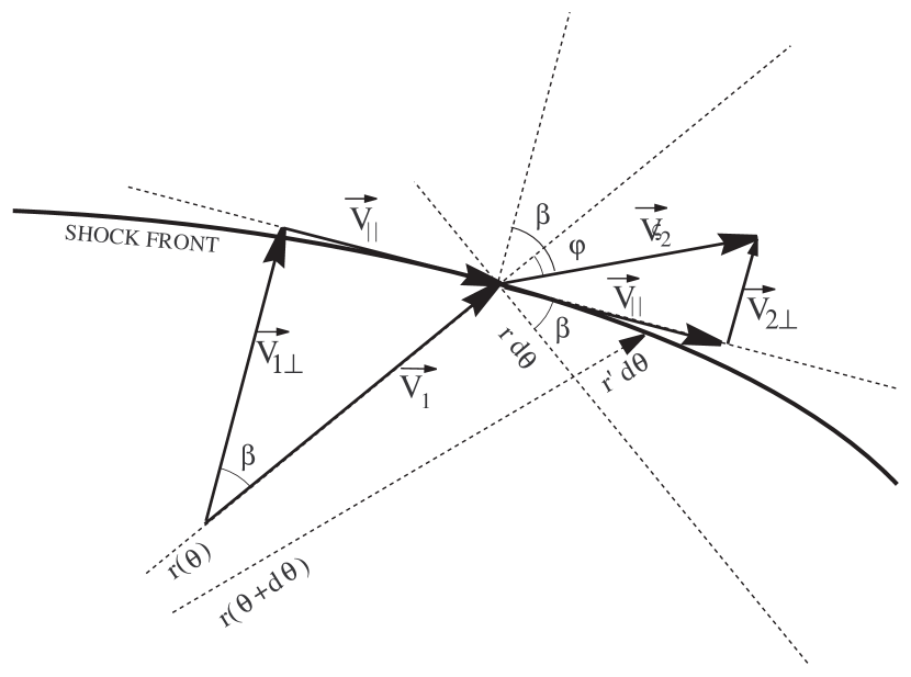
Figure 3: The flow geometry near the shock front.

For weak anisotropy, $v_{\|}\ll 1$. We see from the geometry shown in Fig. 3 that

$$\frac{1}{\gamma_{\|}}\approx 1-{1\over 2}v_{1}^{2}\sin^{2}\beta\approx 1-\frac{v_{1}^{2}}{2}\left(\frac{r_{\mathrm{sh}}^{\prime}(\theta)}{r_{\mathrm{sh}}(\theta)}\right)^{2}.$$ (A19)

Since $r^{{}^{\prime}}_{\mathrm{sh}}\sim\alpha$, the first corrections to $\gamma_{||}$ begin with the terms proportional to $\alpha^{2}$. In the first order of smallness in $\alpha$, we may assume that $\gamma_{||}=1$. The change in the postshock thermodynamic quantities when the flow isotropy breaks down results only from a change in the spatial location of the shock front. To a first approximation, the change in the inclination of the shock surface is negligible.

In that case,

$$p_{2}=\frac{2}{3}\frac{n_{w}}{r_{\mathrm{sh},0}^{2}}\gamma_{w}^{2}mc^{2}\left(1+\alpha\sin^{2}\theta-2\alpha\sum_{m}R_{m}P_{m}(\cos\theta)\right),$$ (A20)

$$\gamma_{2}^{2}=\frac{9}{8},$$ (A21)

$$n_{2}=3\gamma_{0}n_{w}\left(1-2\alpha\sum_{m}R_{m}P_{m}(\cos\theta)\right).$$ (A22)

Hence, we have for $A$ and $S$

$$S=S_{0}\Bigg{(}1+\alpha\sin^{2}\theta{+}{}\\ {}+\left.2/3\alpha\sum_{m}R_{m}P_{m}(\cos\theta)\right),$$

$$A=A_{0}\left(1-2/3\alpha\sum_{m}R_{m}P_{m}(\cos\theta)\right),$$ (A23)

where $A_{0}$ and $S_{0}$ are the constants that are of no interest.

Substituting the expressions for $A$ and $S$ in relation (A.10) yields

$$(u_{s}^{2}-u_{0}^{2})f_{rr}+\frac{1-\eta^{2}}{r^{2}}f_{\eta\eta}-2\frac{u_{0}^{2}}{r}f_{r}=$$ (A24)

$$=\frac{(n_{0}r)^{2}}{\left(n_{\mathrm{sh}}r_{\mathrm{sh}}^{2}u_{\mathrm{sh}}\right){2}}(1-\eta^{2})\left[2\eta\frac{u_{s}^{2}-u_{0}^{2}}{4}\right.-\left.2/3\left(u_{s}^{2}\gamma^{2}-\frac{u_{s}^{2}-u_{0}^{2}}{4}\right)\sum_{m}R_{m}P_{m}^{\prime}(\eta)\right].$$

We seek a solution to Eq. (A.26) in the form

$$f(r,\eta)=\sum_{n}Q_{n}(\eta)f^{(m)}(r),$$ (A25)

where $Q_{m}(\eta)$ are the eigenfunctions of the operator

$$(1-\eta^{2})Q_{m}^{\prime\prime}(\eta)=-m(m+1)Q_{m}(\eta);$$ (A26)

These are

$$Q_{m}(\eta)=(1-\eta^{2})P_{m}^{\prime}(\eta).$$ (A27)

Substituting (A.27) in (A.26) yields

$$(u_{s}^{2}-u_{0}^{2})f^{(m)}_{xx}-\frac{m(m+1)}{x^{2}}u_{s}^{2}f^{(m)}-2\frac{u_{0}^{2}}{x}f^{(m)}_{x}=$$ (A28)

$$={1\over u_{0}^{2}x^{2}}\left[\frac{2}{3}\delta_{2,m}\frac{u_{s}^{2}+u_{0}^{2}}{4}+2/3\left(u_{s}^{2}\gamma^{2}-\frac{u_{s}^{2}-u_{0}^{2}}{4}\right)R_{m}\right],$$

where $x=r/r_{\mathrm{sh},0}$.

The function ${u_{0}}$ was numerically determined from the equations for a polytropic, spherically symmetric postshock flow. This function depends only on one variable $x$. Since the first boundary condition at the shock front is the continuity of $\psi$,

$$f^{(m)}(1)=0.$$ (A29)

The second boundary condition follows from the shock-adiabat relations for an oblique shock wave. Behind the shock,

$$n_{2}u_{2\theta}=-\alpha\frac{r_{\mathrm{sh}}^{2}n_{\mathrm{sh},0}u_{\mathrm{sh}}}{r\sin\theta}\frac{\partial f}{\partial r}.$$ (A30)

We see from Fig. 3 that at $\varphi\ll 1$ and $\beta\ll 1$,

$$\frac{u_{2\theta}}{u_{2r}}=\varphi=-\frac{\alpha}{\sin\theta x}\frac{\partial f}{\partial x},\quad\varphi+\beta=\frac{v_{\|}}{v_{2\bot}}.$$ (A31)

In the first order of smallness in $\alpha$, we have

$$v_{2\bot}=\frac{1}{3},\quad v_{\|}=\beta=\frac{r_{\mathrm{sh}}^{\prime}(\theta)}{r_{\mathrm{sh}}(\theta)}.$$ (A32)

It follows from (A.33, A.34) at $x=1$ that

$$\frac{\partial f}{\partial x}=2(1-\eta^{2})\sum_{m}R_{m}\frac{dP_{m}(\eta)}{d\eta},$$ (A33)

and the second boundary condition for $f^{(m)}$ takes the form

$$\frac{\partial f^{(m)}}{\partial x}\mid_{x=1}=2R_{m}.$$ (A34)

The general solution of Eq. (A.30) with the boundary conditions (A.31, A.36) is

$$f^{(m)}=\delta_{m,2}f^{(m)}_{1}+R_{m}f^{(m)}_{2},$$ (A35)

where $f^{(m)}_{1}$ is the solution of the inhomogeneous equation ( .30) with the right-hand side ${1\over u_{0}^{2}x^{2}}\frac{2}{3}\frac{u_{s}^{2}-u_{0}^{2}}{4}$ and the boundary conditions $f^{(m)}_{i}(1)=0,\quad\frac{\partial f^{(m)}_{i}}{\partial x}\mid_{x=1}=0$. $f^{(m)}_{2}$ is the solution of the same equation with the right-hand side ${1\over u_{0}^{2}x^{2}}{2\over 3}\left(u_{s}^{2}\gamma^{2}-\frac{u_{s}^{2}-u_{0}^{2}}{4}\right)$ and the boundary conditions $f^{(m)}_{2}(1)=0,{\partial f^{(m)}_{2}\over\partial x}=2$. Since the functions $f^{(m)}_{1}$ and $f^{(m)}_{2}$ increase with distance $x$ faster than $x^{4}$, $R_{m}\rightarrow 0$ when $x_{\infty}\rightarrow\infty$ under any boundary condition. Therefore, for all $m\neq 0$ and for $m\neq 2$, we may assume that $R_{m}=0$. This condition physically means that all obstacles that can be in the flow lie far enough from the shock for their influence on the flow near the shock to be ignored.

Figure 4 shows a family of solutions (A.37) for various $R_{2}$. All these solutions satisfy the boundary conditions at the shock. To single out the only solution, we must formulate the boundary conditions far from the shock. It is easy to verify that if there are obstacles in the postshock flow, then the postshock perturbation grows faster than $x^{4}$. In this case, the condition that there are no additional obstacles behind the shock in the presence of anisotropy is the requirement that the perturbation should grow with $x$ more slowly than $x^{4}$, for example, as $x^{3}$. This will take place if the right-hand side of Eq. (A.30) tends to zero as $x$ increases. In turn, it is easy to find that the right-hand side of this equation tends to zero for $R_{2}=-{1\over 3}$. The solution for this value of $R_{2}$ is indicated in Fig. 4 by the solid line. It is the separatrix that separates the solutions tending to $+\infty$ from the solutions tending to $-\infty$ for $x\rightarrow\infty$.

Although the expansion of $f$ includes the terms with $m>1$, we must also determine $R_{0}$, because this term appears in the expansion of $r_{\mathrm{sh}}$ in terms of Legendre polynomials. This coefficient can be easily determined from the condition for the shock location being constant on the rotation axis. The shock front then takes the form

$$r_{\mathrm{sh}}=r_{\mathrm{sh},0}\left(1+\alpha\left({1\over 3}P_{0}-{1\over 3}P_{2}\right)\right)=r_{\mathrm{sh},0}\left(1+{\alpha\over 2}\sin^{2}\theta\right).$$ (A36)

In this solution, the postshock pressure $p_{2}$ is constant along the front and the density varies as

$$n_{2}=3\gamma_{w}n_{w}(1-\alpha\sin^{2}\theta).$$ (A37)

Accordingly, the mean energy of the chaotic particle motion behind the shock front $\epsilon_{2}=3p_{2}/n_{2}$ is

$$\epsilon_{2}={2\over 3}\gamma_{w}mc^{2}(1+\alpha\sin^{2}\theta).$$ (A38)

Thus, as the energy flux density increases along the equator, the shock front is extended along the equatorial plane; the pressure along the front is constant, to a first approximation. The postshock particle density at the equator is lower and their mean thermal energy is higher than those for the particles along the rotation axis. Figure 5 shows streamlines in the flow for $\alpha=0.25$. We see that, in addition to this, the increase in the energy flux density along the equator also causes the bending of the streamlines toward the equator. Initially, this takes place at the shock, where, according to the conditions for an oblique shock wave, the streamlines are pressed to the shock. Subsequently, the streamlines continue to be pressed to the equator. Of course, we cannot talk about the behavior of the solutions far from the shock front, where our solution can yield a qualitatively incorrect result. However, we see that there is one tendency at small distances from the shock front: the bending of the streamlines toward the equator behind the shock.

Translated by V. Astakhov

Figure 4: A family of solutions to Eq. (A.30) Solid line is the solution that corresponds to the absence of additional perturbations in the postshock flow.

Figure 5: The distribution of streamlines for a flow with $\alpha=0.25$. The shock location for isotropic (dashed line) and anisotropic (solid line) flows. The bending of the streamlines at the shock and the further bending of the flow toward the equator result in the flow compression near the equatorial plane.

References

- (1) F. A. Aharonian, A. G. Akhperjanian, J. A. Barrio, et al., Astrophys. J. 539, 317 (2000).
- (2) J. Arons, Astrophys. J. 266, 215 (1983).
- (3) A. M. Atoyan and F. A. Aharonian, Mon. Not. R. Astron. Soc. 278, 525 (1996).
- (4) M. C. Begelman and Z.-Y. Li, Astrophys. J. 397, 187 (1992).
- (5) M. C. Begelman, Astrophys. J. 493, 291 (1998).
- (6) V. S. Beskin, Usp. Fiz. Nauk 167, 690 (1997) [Phys. Usp. 40, 659 (1997)].
- (7) V. S. Beskin, I. V. Kuznetsova, and R. R. Rafikov, Mon. Not. R. Astron. Soc. 299, 341 (1998).
- (8) S. V. Bogovalov, Astron. Astrophys. 349, 1017 (1999).
- (9) S. V. Bogovalov and K. Tsinganos, Mon. Not. R. Astron. Soc. 305, 211 (1999).
- (10) S. V. Bogovalov and F. A. Aharonian, Mon. Not. R. Astron. Soc. 313, 504 (2000).
- (11) S. V. Bogovalov, Astron. Astrophys. 371, 1155 (2001).
- (12) S. V. Bogovalov, Astron. Astrophys. 367, 159 (2001a).
- (13) K. S. Cheng, M. Ruderman, and L. Zhang, Astrophys. J. 537, 964 (2000).
- (14) A. M. Cherepashchuk, Itogi Nauki Tekh., Ser. Astron. 38, 60 (1988).
- (15) F. V. Coroniti, Astrophys. J. 349, 538 (1990).
- (16) J. K Daugherty and A. K. Harding, Astrophys. J. 458, 278 (1996).
- (17) O. C. de Jager and A. K. Harding, Astrophys. J. 396, 161 (1992).
- (18) A. Ferrari, S. Massaglia, G. Bodo, and P. Rossi, in Solar and Astrophysical Magnetohydrodynamic Flows, Ed. by K. Tsinganos (Kluwer, Dordrecht, 1996), p. 607.
- (19) B. M. Gaensler, M. J. Pivovaroff, and G. P. Garmire, Astrophys. J. 556, 107 (2001).
- (20) Y. Gallant, M. Hoshino, A. B. Langdon, et al., Astrophys. J. 391, 72 (1992).
- (21) J. J. Hester, in Proceedings of the International Conference ”Neutron Stars and Pulsars: Thirty Years after the Discovery”, Tokyo, 1997, Ed. by N. Shibazaki et al., p. 431.
- (22) C. F. Kennel and F. V. Coroniti, Astrophys. J. 283, 710 (1984).
- (23) L. D. Landau and E. M. Lifshitz, Course of Theoretical Physics, Vol. 2: The Classical Theory of Fields (Nauka, Moscow, 1973; Pergamon, Oxford, 1975).
- (24) L. D. Landau and E. M. Lifshitz, Course of Theoretical Physics, Vol. 8: Electrodynamics of Continuous Media (Nauka, Moscow, 1982; Pergamon, New York, 1984).
- (25) L. D. Landau and E. M. Lifshitz, Course of Theoretical Physics, Vol. 6: Fluid Mechanics (Nauka, Moscow, 1986; Pergamon, New York, 1987).
- (26) M. Livio, Phys. Rep. 311, 225 (1999).
- (27) Y. Lyubarsky and J. G. Kirk, Astrophys. J. 547, 437L (2001).
- (28) Y. E. Lyubarsky, Mon. Not. R. Astron. Soc. 329, L34 (2002).
- (29) L. Mestel, Mon. Not. R. Astron. Soc. 138, 359 (1968).
- (30) I. F. Mirabel and L. F. Rodrigues, Nature 392, 673 (1998).
- (31) I. Okamoto, Mon. Not. R. Astron. Soc. 185, 69 (1978).
- (32) G. G. Pavlov, O. Y. Kargaltsev, D. Sanwall, and G. P. Garmire, Astrophys. J. 554, L189 (2001).
- (33) M. J. Rees and F. E. Gunn, Mon. Not. R. Astron. Soc. 167, 1 (1974).
- (34) R. W. Romani, Astrophys. J. 470, 469 (1996).
- (35) I. S. Shklovskii, Supernovae (Wiley, New York, 1968).
- (36) T. Tanimori, K. Sakurazawa, S. A. Dazeley, et al., Astrophys. J. 492, L33 (1998).
- (37) C. M. Urri and P. Padovani, Publ. Astron. Soc. Pac. 107, 803 (1995).
- (38) M. C. Weisskopf, J. J. Hester, F. A. Tenant, et al., Astrophys. J. 536, L81 (2000).