Gamma-Ray Burst Neutrino Background and Star Formation History in the Universe

Abstract

We estimate the flux of the GRB neutrino background and compute the event rate at SK and TITAND in the collapsar model, assuming that GRB formation rate is proportional to the star formation rate. We find that the flux and the event rate depend sensitively on the mass-accretion rate. Although the detection of signals from GRBs seems to be difficult by SK, we find that we can detect them by TITAND (optimistically $\sim$ 20 events per year in the energy range $E_{{\overline{\nu}}_{e}}\geq 50$MeV). Therefore, we show that we will obtain the informations on the mass-accretion rate of collapsar by observing the GRB neutrino background, which, in turn, should give us informations on the total explosion energy of GRBs.

I Introduction

Gamma-Ray Burst (GRB) is one of the most mysterious phenomena in the universe. Although there was a great revolution in our understanding on GRBs in 1997 that some of them were proved to be of extragalactic origins [1], there are still a lot of questions and puzzles left on the phenomena. That is why GRBs have been the fascinating targets for astronomers. In fact, there are a lot of interesting and valuable discussions under debate. For example, we have not known what is the origin of GRB. Although this problem has never been settled and still controversial, there are some reports that suggest the physical connections between GRBs and supernovae (SNe) [2]. If the SN/GRB connection is correct, GRBs will be born from the death of massive stars. Then the GRB event rate should trace the star formation history in the universe [3].

The central engine of a GRB is an important but difficult problem to be solved. Although a fireball model [4] is a promising and attractive one, we do not know how the initial condition is. We merely gave it artificially. In the fireball model, since the ratio of baryon number to photon number is required to be extremely small as an initial condition, only a peculiar environment could meet such a condition. As long as we believe the GRB/SN connection, however, a collapsar (failed supernova) model [5] will be one of the convincing candidates as the central engine of a GRB. In the model, much energy is generated by the neutrino heating from an accretion disk surrounding a black hole which is made by the core collapse of a massive star.

On the other hand, total explosion energy of a GRB is also one of the most important problems in the physics of GRBs. Observationally it is well known that there is a large dispersion of total energy of gamma-rays emitted from GRBs [6]. Although the dispersion may become small when we consider the beaming effects [7], after all we do not know the total explosion energy of the system that generates a GRB only by the gamma-ray observations. In the theoretical side, the total explosion energy in the collapsar model is also not estimated clearly, and only a rough estimate is reported as a result of the numerical computations [9]. Therefore, to know the total explosion energy, we require the multi-dimension numerical hydrodynamical computations including the microphysics of neutrino heating in future, which is, of course, a laborious task to be performed.

Are there observations which give us new clues to know how a GRB is produced? In this study, we point out that the GRB neutrino background may be detected in a large water Cherenkov neutrino detector such as Super-Kamiokande (SK) and TITAND which is proposed as a next-generation plan of the multi-megaton water Cherenkov detector [8]. We also stress that this signal should give us valuable informations on GRBs, such as the total explosion energy and/or event rate of GRBs. The reason is as follows. In this study, we assume that the origins of GRBs are massive stars. Thus, the event rate of GRBs should trace the star formation history in the universe. Since we adopt the collapsar model here, we can assume that the central engine of a GRB is the neutrino heating from an accretion disk surrounding the central black hole. We show that the total number of neutrinos emitted from a GRB is very sensitive to the mass-accretion rate $\dot{M}$ which is difficult to estimate only from the existing theoretical models. However, we can obtain the informations of the mass-accretion rate by observing the GRB neutrino background. We also derive an approximate relationship between the total explosion energy and the mass-accretion rate of a GRB. Namely, although we cannot determine the total explosion energy only from the gamma-ray observations, we can obtain informations of it by observing the GRB neutrino background. That is an important clue to understand GRBs. In this study we find that the GRB neutrino background may be detected within $\sim$ 10 yrs by TITAND as long as the average mass-accretion rate among GRBs is $\dot{M}\gtrsim$ a few $M_{\odot}$ s^-1, and the probability that one collapsar generates a GRB is $f$ $\sim$ 0.5 – 1.0.

Here we outline the organization of this paper. In section II, we explain the formulations in this study. Results are shown in section III. Discussions are given in section IV. Summary and conclusion are presented in section V.

II Formulation

A GRB formation history

First we assume that the rate of GRBs traces the global star formation history of the universe, $R_{\rm GRB}(z)\propto R_{\rm SFR}$. Although a number of workers have modeled the expected evolution of the cosmic SFR with redshift, there are some uncertainties (in particular, at high redshift $z\geq 1$), and further observations are required to determine the cosmic SFR. In this study, we use the three different parameterizations of the global star formation rate per comoving volume in an Einstein-de Sitter universe to take into account the uncertainty of the cosmic SFR which is derived by Ref. [3]. They are

$$R_{\rm SF1}(z)=0.3h_{65}\frac{\exp(3.4z)}{\exp(3.8z)+45}\;M_{\odot}\rm yr^{-1}Mpc^{-3},$$ (1)

$$R_{\rm SF2}(z)=0.15h_{65}\frac{\exp(3.4z)}{\exp(3.4z)+22}\;M_{\odot}\rm yr^{-1}Mpc^{-3},$$ (2)

and

$$R_{\rm SF3}(z)=0.2h_{65}\frac{\exp(3.05z-0.4)}{\exp(2.93z)+15}\;M_{\odot}\rm yr^{-1}Mpc^{-3},$$ (3)

where $h_{65}=H_{0}/\rm 65\;km\;s^{-1}\;Mpc^{-1}$.

Assuming that massive stars with masses larger than $\sim 35M_{\odot}$ explode as GRBs [9] [10], GRB-rate density $R_{\rm GRB}$ can then be estimated by multiplying the selected SFR by the coefficient

$$f\times\frac{\int^{125}_{35}dm\;\phi(m)}{\int^{125}_{0.4}dm\;m\phi(m)}=1.5\times 10^{-4}\left(\frac{f}{0.1}\right)M_{\odot}^{-1},$$ (4)

where $\phi(m)$ is the initial mass function (IMF) and $m$ is the stellar mass in solar units. In this study, the Salpeter’s IMF ($\phi(m)\propto m^{-2.35}$) is adopted throughout. Here we assumed that one tenth of the collapsars whose mass range is in (35 – 125)$M_{\odot}$ are accompanied with GRBs ($\equiv f$). The validity of this assumption and the detailed discussions are presented in section IV. We label these models as GRBR1, GRBR2, and GRBR3, respectively. For comparison, we use the SN-rate density $R_{\rm SN}$ by multiplying the selected SFR by the coefficient

$$\frac{\int^{35}_{8}dm\;\phi(m)}{\int^{125}_{0.4}dm\;m\phi(m)}=1.2\times 10^{-2}M_{\odot}^{-1}.$$ (5)

As for the energy spectrum of ${\overline{\nu}}_{e}$ of SNe, the Fermi-Dirac distribution with zero chemical potential is used (see Figs 9– 11), which have the same luminosity with the numerical model [11].

In the flat universe, i.e., when the density parameter is $\Omega=\Omega_{M}+\Omega_{\Lambda}=1$ with the non-relativistic matter density ($\Omega_{M}\sim 0.3$) and the $\Lambda$ term ($\Omega_{\Lambda}\sim 0.7$), the star formation rate is given by [3]

$$R_{\rm SF}(z;\Omega_{M}.\Omega_{\Lambda},h_{65})=h_{65}\frac{\sqrt{((1+\Omega_{M}z))(1+z)^{2}-\Omega_{\Lambda}(2z+z^{2})}}{(1+z)^{3/2}}R_{\rm SF}(z;1,0,1),$$ (6)

where $z$ is redshift. In Fig. 1, we show the GRB rates as a function of the redshift.

B Accretion disk model

1 Energy Spectrum

In the collapsar model, neutrinos are mainly generated at the inner-most region of an accretion disk which is formed around the central black hole. Thus we estimate the energy spectrum of neutrinos using an analytical shape of the accretion disk. Popham et al. (1999) proposed an accretion-disk model including the effects of general relativity as a collapsar model [12]. The model in Ref. [12] and the numerically computed collapsar model [9] are fitted well by the analytical shape of the accretion disk in Ref [12, 13] . We use it in this study. Then, the density [g cm^-3], the temperature [MeV] and the disk thickness [cm] are fitted as follows (see Ref. [15] for details).

$$\rho=8.23\times 10^{8}\left(\frac{M}{3M_{\odot}}\right)^{-1.7}\left(\frac{\dot{M}}{0.1M_{\odot}{\rm s}^{-1}}\right)^{1.03}\frac{1}{\displaystyle{\left(\frac{r}{r_{s}}\right)^{1.07}\left(1+\left(\frac{r}{r_{s}}\right)\right)^{0.76}}},$$ (7)

$$T=2.3\times\left(\frac{M}{3M_{\odot}}\right)^{-0.2}\left(\frac{\dot{M}}{0.1M_{\odot}{\rm s}^{-1}}\right)^{0.108}\frac{1}{\displaystyle{\left(\frac{r}{r_{s}}\right)^{0.425}\left(1+\left(\frac{r}{r_{s}}\right)\right)^{0.21}}},$$ (8)

$$H=5.8\times 10^{6}\left(\frac{M}{3M_{\odot}}\right)^{0.9}\left(\frac{\dot{M}}{0.1M_{\odot}{\rm s}^{-1}}\right)^{-0.0183}\frac{1}{\displaystyle{\left(\frac{r}{r_{s}}\right)^{-1.66}\left(1+\left(\frac{r}{r_{s}}\right)\right)^{0.3867}}},$$ (9)

where $M$ is the mass of the central black hole, $r$ is the radial coordinate, and $r_{s}$ (= 10⁷cm) is the core radius, respectively. Note that the Schwarzshild radius is $\simeq 8.862{\rm km}(M/3M_{\odot})$. In Ref. [12], they assumed that the mass of the central black hole is constant. In this study, however, to estimate the total energy of neutrinos we consider the effects that the mass of the central black hole becomes larger with time by accretions.

When we know the density and the temperature in the neutrino emitting region, we can estimate the emissivity of neutrinos ($\rm cm^{-3}sec^{-1}MeV^{-1}$) in the accretion disk. The total emissivity of ${\overline{\nu}}_{e}$ is represented by two terms:

$$\frac{d^{2}n_{{\overline{\nu}}_{e}}}{dtdE_{{\overline{\nu}}_{e}}}=\frac{d^{2}n^{eN}_{{\overline{\nu}}_{e}}}{dtdE_{{\overline{\nu}}_{e}}}+\frac{d^{2}n^{e^{+}e^{-}}_{{\overline{\nu}}_{e}}}{dtdE_{{\overline{\nu}}_{e}}},$$ (10)

where $E_{{\overline{\nu}}_{e}}$ is energy of ${\overline{\nu}}_{e}$. For $n+e^{+}\rightarrow p+{\overline{\nu}}_{e}$, the emissivity of ${\overline{\nu}}_{e}$ is represented by

$$\frac{d^{2}n_{{\overline{\nu}}_{e}}^{eN}}{dtdE_{{\overline{\nu}}_{e}}}(E_{{\overline{\nu}}_{e}})= \frac{G_{F}^{2}}{2\pi^{3}}(1+3g_{A}^{2})n_{n}E_{{\overline{\nu}}_{e}}^{2}\sqrt{\left(E_{{\overline{\nu}}_{e}}-Q\right)^{2}-m_{e}^{2}}\left(E_{{\overline{\nu}}_{e}}-Q\right)\frac{1}{e^{(E_{{\overline{\nu}}_{e}}-Q)/T}+1},$$ (11)

where $G_{F}$ is Fermi coupling constant, $g_{A}$ is the axial vector coupling constant of the nucleon which is normalized by the experimental value of neutron lifetime $\tau_{n}\simeq 886.7$ s [16], $n_{n}$ is number density of neutron, Q $\simeq$ 1.29 MeV, and $m_{e}$ is electron mass. For $e^{-}+e^{-}\rightarrow\nu_{e}+{\overline{\nu}}_{e}$, we obtain

$$\frac{d^{2}n_{{\overline{\nu}}_{e}}^{e^{+}e^{-}}}{dtdE_{{\overline{\nu}}_{e}}}(E_{{\overline{\nu}}_{e}})= \frac{G_{F}^{2}}{9\pi^{4}}(C_{V}^{2}+C_{A}^{2})E_{{\overline{\nu}}_{e}}^{3}\frac{1}{e^{E_{{\overline{\nu}}_{e}}/T}+1}T^{4}\int^{\infty}_{m_{e}/T}\frac{(\epsilon^{2}-(m_{e}/T)^{2})^{3/2}}{e^{\epsilon}+1}d\epsilon,$$ (12)

where $C_{V}=1/2+2\sin^{2}\theta_{W}$, $C_{A}$ = 1/2, and $\sin^{2}\theta_{W}\simeq 0.231$ is Weinberg angle [16], and we assume $T\gg m_{e}$. We plot them in Fig. 2 in the case that $T=$ 5MeV and $\rho=10^{10}{\rm g}\cdot{\rm cm}^{-3}$.

Using Eqs. (7), (8) and (9), we obtain the integrated energy spectrum of ${\overline{\nu}}_{e}$,

$$\frac{dn}{dE_{{\overline{\nu}}_{e}}}(E_{{\overline{\nu}}_{e}})=\int_{0}^{\Delta t}dt\int_{T\geq 1{\rm MeV}}dV_{a}\frac{d^{2}n_{{\overline{\nu}}_{e}}}{dtdE_{{\overline{\nu}}_{e}}}(E_{{\overline{\nu}}_{e}}),$$ (13)

where $\int dV_{a}$ denotes the integration in the volume of the emitting region in accretion disk where the temperature is high enough to produce neutrinos, i.e., $T\geq 1$ MeV, $\int dt$ denotes the integration of time $t$, and $\Delta t\equiv M_{a}/\dot{M}$ is the duration of the accretion ($M_{a}$ is the mass of the progenitor). Here we assume that the time evolution of the mass of the central black hole is given by

$$M=M_{i}+\dot{M}t,$$ (14)

where $M_{i}$ is the initial value of $M$. In this study, $M_{i}$ is set to be 3$M_{\odot}$. In Fig. 3 we plot the obtained energy spectrum of ${\overline{\nu}}_{e}$ emitted from the accretion disk in unit energy [${\rm MeV}^{-1}$].

Here we define the time-dependent luminosity of $\nu_{e}$ and ${\overline{\nu}}_{e}$ by

$$L_{\nu}(t)=\int_{T\geq 1{\rm MeV}}dV_{a}\left(\int dE_{{\overline{\nu}}_{e}}\frac{d^{2}n_{{\overline{\nu}}_{e}}}{dtdE_{{\overline{\nu}}_{e}}}(E_{{\overline{\nu}}_{e}})+\int dE_{{\nu_{e}}}\frac{d^{2}n_{{\nu_{e}}}}{dtdE_{{\nu_{e}}}}(E_{{\nu_{e}}})\right),$$ (15)

where $dn_{\nu_{e}}/dtdE_{{\nu_{e}}}$ is the total emissivity of $\nu_{e}$ with their energy $E_{{\nu_{e}}}$, and we assume it is approximately equal to $dn_{{\overline{\nu}}_{e}}/dtdE_{{{\overline{\nu}}_{e}}}$. In addition, we define the total energy of $\nu_{e}$’s and ${\overline{\nu}}_{e}$’s emitted from a collapsar,

$$Q_{\rm tot}=\int_{0}^{\Delta t}L_{\nu}(t)dt.$$ (16)

We see from Eq. (8) that as the mass of the central black hole grows, the temperature becomes lower, and the flux of neutrinos decreases. In Fig. 4, we show the duration ($\equiv\Delta t_{\nu,{\rm emit}}$) which is defined as the e-folding time of the time-dependent luminosity in Eq. (15). This almost corresponds to the timescale in which the temperature at the innermost region of the accretion disk becomes lower than $\sim$ 1 MeV. Namely this will approximately reflect the timescale of a GRB.

Now we investigate the dependence of the energy spectrum of anti-electron neutrino on the mass-accretion rate ($\dot{M}$). The mass-accretion rate is theoretically not known while the numerical simulations have been performed, because there are uncertainties on the viscosity of the accretion disk and angular momentum of the progenitor. In Fig. 5, we show the energy spectrum for the case of $\dot{M}$ = 0.01$M_{\odot}$ s^-1, 0.1$M_{\odot}$ s^-1, 1$M_{\odot}$ s^-1, 5$M_{\odot}$ s^-1, and 10$M_{\odot}$ s^-1. The energy spectrum is represented as $E_{{\overline{\nu}}_{e}}^{2}dn/dE_{{\overline{\nu}}_{e}}$ [MeV] because the cross section of the reaction $p+{\overline{\nu}}_{e}\to n+e^{+}$ is proportional to the square of the energy. It is clearly shown that the energy spectrum becomes hard, and intensity becomes large as the mass-accretion rate increases. This is because the temperature at the inner region of the accretion disk becomes higher. Here we have to give some comments on the application limit for the present accretion disk model in this study. High energy electron-positron pairs whose energies are greater than $\sim 100$MeV produce muons and charged pions, which, in turn, decay into low energy leptons. Such microphysics is not included in the present model. The influence might become important for the high accretion rate model. In addition, as the density becomes large, the assumption that the neutrinos are optically thin might become to break down [12]. For example, the opacity of electron neutrino ($\tau$) at the inner most region of the accretion disk is estimated as [17]

$$\tau = \int\frac{1}{2}N_{A}\rho\sigma dr$$ (17)

$$\sim 1.6\times 10^{-9}T_{\rm MeV}^{2}\rho_{10}H$$ (18)

$$\sim 4.1\times 10^{-3}\left(\frac{3M_{\odot}}{M}\right)^{1.5}\left(\frac{\dot{M}}{0.1M_{\odot}s^{-1}}\right)^{1.23}\frac{1}{\displaystyle{\left(\frac{r}{r_{s}}\right)^{0.26}\left(1+\left(\frac{r}{r_{s}}\right)\right)^{1.57}}},$$ (19)

where $N_{A}$ is the Avogadro’s number, $\sigma$ is the cross section of the neutrino off a nucleon, $\rho_{10}$ is the density normalized by 10¹⁰ g cm^-3. Therefore, $\tau$ may comparably become unity if $\dot{M}$ is approximately $10M_{\odot}$ s^-1, $r\sim r_{g}$, and $M\sim 3M_{\odot}$. From the above considerations, models with high accretion rate ($\dot{M}\sim 10M_{\odot}$ s^-1) may be the extreme cases.

In Fig. 6, we show the average neutrino luminosity which is defined by

$${\overline{L}}_{\nu}=Q_{\rm tot}/\Delta t_{\nu,{\rm emit}}.$$ (20)

For comparison, in the figure we also show the result of Popham et al. (1999). The uncertainty of their results comes from the Kerr parameter of the central black hole ($a=0$ – 0.5). From the figure, we find that our simple formula reproduce their results fairly well in wide range of mass-accretion rate. At high mass-accretion rate ($\dot{M}\sim 10M_{\odot}$ s^-1), our formula may overestimate the neutrino luminosity by a factor of three. As shown below (see section III), however, we also compute the GRB neutrino background in such models as extreme cases. In future, improvements of the accretion model will enhance the predictability of the flux of GRB neutrino background.

The event rates of ${\overline{\nu}}_{e}$ expected in water Cherenkov detectors is represented by

$$\frac{dR}{dE_{e^{+}}}=\frac{N_{p}}{4\pi D^{2}}\sigma_{p{\overline{\nu}}_{e}}(E_{e^{+}})\frac{dn}{dE_{{\overline{\nu}}_{e}}}(E_{e^{+}}),$$ (21)

where $E_{e^{+}}=E_{{\overline{\nu}}_{e}}-Q$ is the energy of the positron which is scattered through $p+{\overline{\nu}}_{e}\rightarrow n+e^{+}$ in the detector, $\sigma_{p{\overline{\nu}}_{e}}=\frac{G_{F}^{2}}{\pi}(1+3g_{A}^{2})E_{e^{+}}\sqrt{E_{e^{+}}^{2}-m_{e}^{2}}$ is the cross section of the process, and $D$ is the distance from the Earth to the collapsar. $N_{p}$ is the number of proton in the detector, e.g., $N_{p}\simeq 1.5\times 10^{33}$ for SK. Thus the total event rate is estimated by the integration,

$$R=\int dE_{e^{+}}\frac{dR}{dE_{e^{+}}}.$$ (22)

2 Estimate for the total explosion energy

It is reported that the energy deposition rate becomes as large as $\sim 10^{51}$ erg s^-1 by the $\nu{\overline{\nu}}$ pair annihilation [12]. In their studies, they computed the energy deposition rate considering the shape of the accretion disk. Their results are shown in Fig. 7 as a shaded region. Here the efficiency of $\nu_{e}{\overline{\nu}}_{e}$ pair annihilations is defined as $\epsilon\equiv Q_{e+e-}/Q_{\rm tot}$, where $Q_{e+e-}$ is the total deposited energy. Their results are fitted well as

$$\epsilon=1.32\times 10^{-2}\left(\frac{\dot{M}}{1M_{\odot}s^{-1}}\right)^{1.56},$$ (23)

which is also shown in Fig. 7. In this study, we use this fitting formula to estimate the explosion energy of a GRB. Then, we obtain the total deposited energy by $Q_{e^{+}e^{-}}$ = $\epsilon Q_{\rm tot}$. In Fig. 8, the total energy of emitted neutrinos ($Q_{\rm tot}$) and the total deposited energy ($Q_{e+e-}$) are shown as a function of the mass-accretion rate. Since the total explosion energy of SN1998bw is reported to be $\sim 10^{52}$ erg [9], we find that it corresponds to the mass-accretion rate $\sim(1-2)M_{\odot}s^{-1}$ in Fig. 8.

For simplicity, we ignored the heating process from $\nu_{\mu}{\overline{\nu}}_{\mu}$ and $\nu_{\tau}{\overline{\nu}}_{\tau}$ pair annihilations in this computation because the effect is much smaller than $\nu_{e}{\overline{\nu}}_{e}$ pair annihilation. The reason is as follows. In the electromagnetic thermal bath, $\nu_{\mu}{\overline{\nu}}_{\mu}$ and $\nu_{\tau}{\overline{\nu}}_{\tau}$ pairs are produced from $e^{+}e^{-}$ pair annihilations only through the neutral current interaction. In addition, $\nu_{\mu}{\overline{\nu}}_{\mu}$ and $\nu_{\tau}{\overline{\nu}}_{\tau}$ pairs annihilate into $e^{+}e^{-}$ pairs only through the neutral current interaction. On the other hand $\nu_{e}{\overline{\nu}}_{e}$ pairs are produced through both the charged and neutral currents and annihilate into $e^{+}e^{-}$ pairs correspondingly through the same process. Then, compared with the case of $\nu_{e}{\overline{\nu}}_{e}$, the efficiency of the heating from $\nu_{\mu}{\overline{\nu}}_{\mu}$ and $\nu_{\tau}{\overline{\nu}}_{\tau}$ pairs in the electromagnetic thermal plasma is just within $10\%$ of the total, even if the $\nu{\overline{\nu}}$ pair production from $e^{+}e^{-}$ pair annihilation dominates all the other processes of neutrino production.

C GRB neutrino background

In order to get the differential number flux of back ground neutrinos, first we compute the present number density of the background neutrinos per unit neutrino energy, $dn(E_{{\overline{\nu}}_{e}})/dE_{{\overline{\nu}}_{e}}$ in Eq. (13). The contribution of the neutrinos emitted in the interval of the redshift $z\sim z+dz$ is given as

$$dN_{\nu}(E_{{\overline{\nu}}_{e}})=R_{\rm GRB}(z)\frac{dt}{dz}dz\frac{dn(E_{{\overline{\nu}}_{e}}^{\prime})}{dE_{{\overline{\nu}}_{e}}^{\prime}}(1+z)dE_{{\overline{\nu}}_{e}},$$ (24)

where $E_{{\overline{\nu}}_{e}}^{\prime}=(1+z)E_{{\overline{\nu}}_{e}}$. It is noted that $R_{\rm GRB}$ is GRB rate per comoving volume, and the effect of the expansion of the universe is taken into account in Eq. (24). The Friedmann equation gives the relation between $t$ and $z$ as follows:

$$\frac{dz}{dt}= - H_{0}(1+z)\sqrt{(1+\Omega_{M}z)(1+z)^{2}-\Omega_{\Lambda}(2z+z^{2})}.$$ (25)

We now obtain the differential number flux of GRB, $dF_{\nu}(E_{{\overline{\nu}}_{e}})/dE_{{\overline{\nu}}_{e}}$, by using the relation $dF_{\nu}(E_{{\overline{\nu}}_{e}})/dE_{{\overline{\nu}}_{e}}=cdN_{\nu}(E_{{\overline{\nu}}_{e}})/dE_{{\overline{\nu}}_{e}}$:

$$\frac{dF_{\nu}}{dE_{{\overline{\nu}}_{e}}}= \frac{c}{H_{0}}\int^{z_{\rm max}}_{0}R_{\rm GRB}(z)\frac{dn((1+z)E_{{\overline{\nu}}_{e}})}{dE_{{\overline{\nu}}_{e}}}\frac{dz}{\sqrt{(1+\Omega_{M}z)(1+z)^{2}-\Omega_{\Lambda}(2z+z^{2})}}$$ (26)

III Results

The differential number flux of GRB neutrinos is shown in Figs. 9, 10 and 11. As for the GRB formation history, GRBR1, GRBR2, and GRBR3 are assumed, respectively. It is found that the differential number flux is similar with each other even if the different star formation history is adopted. That is because the energy of neutrinos from high-z GRBs is redshifted as $\propto 1/(1+z)$, and the volume containing high-z GRBs is relatively small $\propto 1/\sqrt{(1+\Omega_{M}z)(1+z)^{2}-\Omega_{\Lambda}(2z+z^{2})}$ as given in Eq. (26). Thus, we show the results only for GRBR3 below. On the other hand, we can see clearly that the differential number flux becomes larger as the mass-accretion rate increases. In particular, in high accretion model such as $\dot{M}=5M_{\odot}$, the intensity of the GRB neutrino background is larger than that of SN neutrino background in the energy region $E_{{\overline{\nu}}_{e}}\geq 50$MeV. As discussed below, in such a high energy region, the neutrino background will be obscured by the noise from the atmospheric neutrino background (ANB). As the event number increases, however, we will have statistically sufficient data, and the signals from GRBs will dominate the statistical error of ANB. In the next section we estimate the time required to detect the signals from GRB (see also Table III). Note that at the energy which is larger than $50$MeV, the signals from GRBs dominate the noise of electrons from the decay of invisible muons because their spectrum has a steep cut-off at $50$MeV. In the next section, we will discuss them in detail.

The event rates at SK are shown in Fig. 12 in units of yr^-1 MeV^-1 for various mass-accretion rates. For event rates, increasingly we cannot discriminate among the three models of the star formation history because the cross section of $p+{\overline{\nu}}_{e}\rightarrow n+e^{+}$ is proportional to the square of the neutrino energy ($\propto E_{{\overline{\nu}}_{e}}^{2}$), and the relative contribution of low energy neutrinos to the event rate is small. Therefore, irrespective of the differences among the models of the star formation history, we can expect the event rate of GRB neutrino background as a function of mass-accretion rate. Namely the informations on the average mass-accretion rate will be obtained from such an observation, which, in turn, should give us informations on the total explosion energy of a GRB (see Fig. 8). They are, of course, never obtained only by the gamma-ray observations.

In Fig. 13, we show the dependence of the event rates on the probability $f$ that one collapsar generates a GRB in the case of $\dot{M}=10M_{\odot}$ s^-1. It is clear that the signals from GRBs dominate those from SN for $E_{\bar{\nu}_{e}}\geq 30$MeV in the case of $f=1.0$. However, the noise from the atmospheric neutrinos obscures the signals of GRBs even if we adopt the high value of $f$ (=1.0). In the next section, we discuss the detectability of the signals of the GRB neutrino background as a significant deviation from the statistical error of ANB.

To estimate the event rates more realistically, we should consider the effects of neutrino oscillation. The flavor eigen states $\nu_{\alpha}$ ($\alpha,=e,\mu,$ and $\tau$) are related with the mass eigen states $\nu_{i}$ (“$i$” = 1, 2, and 3) by the mixing matrix $U$ as $\nu_{\alpha}=\sum_{i}U_{\alpha i}\nu_{i}$. Then, we parameterize it by

$$U=\left(\begin{array}[]{ccc}c_{13}c_{12}&c_{13}s_{12}&s_{13}\\ -c_{23}s_{12}-s_{23}s_{13}c_{12}&c_{23}c_{12}-s_{23}s_{13}s_{12}&s_{23}c_{13}\\ s_{23}s_{12}-c_{23}s_{13}c_{12}&-s_{23}c_{12}-c_{23}s_{13}s_{12}&c_{23}c_{13}\end{array}\right),$$ (30)

with $s_{ij}=\sin\theta_{ij}$ and $c_{ij}=\cos\theta_{ij}$, where we ignored the CP phase in the lepton sector. In general, the probability of the vacuum oscillation from a flavor $\nu_{\alpha}$ to a flavor $\nu_{\beta}$ is represented by

$$P(\nu_{\alpha}\to\nu_{\beta})=\langle\nu_{\beta}|\nu_{\alpha}(t)\rangle=\sum_{i}|U_{\beta i}|^{2}|U_{\alpha i}|^{2}+2Re\sum_{i>j}U_{\beta i}U_{\beta j}^{*}U_{\alpha i}^{*}U_{\alpha j}e^{-i\frac{L}{2E_{\nu}}\delta m^{2}_{ij}},$$ (31)

where $L$ is the distance from the source to the Earth (= $ct$), $E_{\nu}$ is the neutrino energy, and the mass difference is defined by $\delta m^{2}_{ij}\equiv m_{j}^{2}-m_{i}^{2}$. For simplicity, here we assume the normal hierarchy of neutrino masses, $m_{1}<m_{2}<m_{3}$. The results of recent oscillation experiments are as follows. The solar neutrino data favor the Large Mixing Angle solution ($0.6\leq\sin^{2}2\theta_{12}\leq 0.98$), and $2\times 10^{-5}{\rm eV}^{2}\leq\delta m^{2}_{12}\leq 4\times 10^{-4}{\rm eV}^{2}$ at 3$\sigma$ C.L. [18]. The atmospheric neutrino data also imply the large mixing ($\sin^{2}2\theta_{23}\geq 0.85$), and $1.1\times 10^{-3}{\rm eV}^{2}\leq\delta m^{2}_{23}(\simeq\delta m^{2}_{13})\leq 5\times 10^{-3}{\rm eV}^{2}$ at 99 $\%$ C.L. [19]. The CHOOZ reactor experiment shows that $\sin^{2}2\theta_{13}\leq 0.1$ at 95 $\%$ C.L [20]. Then, the above data tells us that $\delta m^{2}_{12}\ll\delta m^{2}_{23}\sim\delta m^{2}_{13}$.

Adopting the above data, we can assume that the mixing matrix is approximately simplified into

$$U\simeq\left(\begin{array}[]{ccc}\sqrt{2}/2&\sqrt{2}/2&0\\ -1/2&1/2&\sqrt{2}/2\\ 1/2&-1/2&\sqrt{2}/2\end{array}\right).$$ (35)

Because neutrinos propagate for long distances, the second term in Eq. (31) is averaged and becomes zero. Then, we have

$$P({{\overline{\nu}}_{e}\to{\overline{\nu}}_{e}}) = 1/2,$$ (36)

$$P({{\overline{\nu}}_{\mu}\to{\overline{\nu}}_{e}}) = 1/4,$$ (37)

$$P({{\overline{\nu}}_{\tau}\to{\overline{\nu}}_{e})} = 1/4.$$ (38)

If we choose the inverted hierarchy, i.e., $\delta m^{2}_{32}\ll\delta m^{2}_{21}\simeq\delta m^{2}_{31}$, we only interchange the roles of $m_{1}$ and $m_{3}$ in Eq. (30). Namely we only interchange the first and third columns of $U$. Even then, it is remarkable that the results in Eq. (36), (37), and (38) are not changed at all.

In Fig. 14, we show the event rate as a function of $E_{{\overline{\nu}}_{e}}$ at SK in which we consider the effects of the neutrino oscillation for $\dot{M}=10M_{\odot}$. It is noted that the flux of ${\overline{\nu}}_{e}$ becomes lower as a result of the neutrino oscillation. That is because ${\overline{\nu}}_{\mu}$ and ${\overline{\nu}}_{\tau}$ are produced only through the $e^{+}e^{-}$ pair annihilation.

IV Discussions

We consider the detectability of the neutrino background from GRBs. In the energy range $E\leq 50$MeV, the neutrino background is obscured by the events of the electrons which come from the decay of invisible muons [21]. The spectrum of the electrons is given by $dN/dE_{e}=(G_{F}^{2}/12\pi^{3})m_{\mu}^{2}E_{e}^{2}(3-4E_{e}/m_{\mu}),$ where $m_{\mu}$ is the muon mass, and $E_{e}$ is the electron (positron) energy. The event rate of the electrons from the invisible muons at SK is about $\sim$ 1 in units of yr^-1 MeV^-1 in the energy range $50\geq E_{{\overline{\nu}}_{e}}\geq 20$MeV [11]. Thus, signals of GRB neutrino background are smaller than those of electrons from invisible muons in the range. In addition, the signals from SN neutrino background will basically dominate those of GRB neutrino background in the energy range. On the other hand, the spectrum of electrons from the invisible muons has a steep cut-off at about 50 MeV because the maximum energy of the emitted electrons is about half of the muon mass. Thus, as mentioned above, the signal from GRBs becomes larger than the noise from invisible muons in the energy range $E_{{\overline{\nu}}_{e}}\geq 50$MeV. In the case of the high mass-accretion rate such as $\dot{M}\gtrsim 5M_{\odot}$, the signals of the GRB neutrino background are larger than those of SN neutrino background in the energy region. However, the severest noise comes from the atmospheric neutrinos. In Table I, we show the event rate (yr^-1) of ANB and its statistical error in SK/TITAND in the energy regions $E_{\bar{\nu}_{e}}$ = (50 – 60)MeV and $E_{\bar{\nu}_{e}}\geq$ 50MeV [22, 23]. TITAND is proposed as a next-generation plan of the multi-megaton water Cherenkov detector [8]. The first phase of TITAND is planed to be with 2 Mt water inside. Thus, the event rate becomes approximately one hundred times larger than SK.

For comparison, we show the event rates from the GRB neutrino background at SK/TITAND in Table II for various models. The third column of the table represents whether we consider the effects of the neutrino oscillation or not. ’Yes’ means that the effects of the neutrino oscillation are taken into account. It is apparent that the signals from GRB are smaller than the noise from ANB. As the event number increases, however, we will have statistically sufficient data, and the signals from GRBs will dominate the statistical error of ANB. Namely, then we can definitely detect the signals of the GRB neutrino background as a significant deviation from the statistical error of ANB. The time (yr) required to marginally distinguish the signals from the noise is computed by $t=N/S^{2}$, where $N$ is the noise (yr^-1) from ANB and $S$ is the signals from GRBs (yr^-1). In Table III, we show the time required to detect the signal of GRBs at SK/TITAND for the energy range $E$ = (50 – 60) MeV and $E\geq 50$ MeV. From the table, we find that we can detect the signals within $\sim$10 years at TITAND in the case that the mass-accretion rate is (5 – 10$M_{\odot}$ s^-1) and $f$ is (0.5 – 1). Although it seems to take a long time to detect the signals from GRBs for the cases in which the conservative parameter sets are adopted, constraints for optimistic parameter sets will be obtained by the observations of TITAND. Of course, a larger water Cherenkov detector than TITAND will detect the signals from GRBs more immediately even if the GRBs obey the conservative parameters.

In this study, we have mainly assumed that one tenth of collapsars whose mass range are in (35 – 125)$M_{\odot}$ are accompanied with GRBs. Here we investigate the validity of the assumption. The locally observed value for the SN rate is in the range $R_{\rm SN}=(1.4\pm 0.5)\times 10^{-4}h_{0.7}^{3}$ yr^-1 Mpc^-3, where $h=H_{0}/$(100 km s^-1 Mpc^-1) [24]. On the other hand, it is reported that the GRB rate at $z=0$ is $2.4\times 10^{-9}h_{0.7}^{3}$ yr^-1 Mpc^-3 using the BATSE data catalog [25]. On the other hand, we assumed that the ratio of the collapsar rate to SN rate is $\sim 0.13$ using Eqs. (4) and (5). Thus, we estimate that the collapsar rate at $z=0$ is $1.8\times 10^{-5}h_{0.7}^{3}$ yr^-1 Mpc^-3. Adopting the beaming factor is $d\Omega\sim 4\pi\times 10^{-3}$, and the probability that one collapsar generates a GRB is $f=0.1$, we estimate the GRB rate at $z=0$:

$$R_{\rm GRB}=1.8\times 10^{-9}\left(\frac{f}{0.1}\right)\left(\frac{d\Omega}{4\pi\times 10^{-3}}\right)\left(\frac{h}{0.7}\right)^{3},$$ (39)

in units of $\rm yr^{-1}\ Mpc^{-3}$ which is consistent with the previous work. At present, the average beaming angle is not determined precisely except for some observations that suggest it is several degree [7]. Therefore, we leave the value of $f$ as a free parameter at present. In addition, the previous works on the GRB formation rate would have a lot of uncertainties since only the BATSE data catalog is used in these analyses, and the average luminosity of GRBs is adopted to fit the model. More precise data on the beaming angle and on the GRB formation rate (for example, by using the peak-lag relation [26]) will give us informations on the probability $f$. Then, our predictions of GRB neutrino background become more correct.

In this study, we have assumed that GRB formation rate is proportional to the star formation rate in the universe. If this assumption is not correct, of course, the resulting energy spectrum will also be changed. Therefore, on the contrary, when we observe the differential flux of GRB neutrino background, we will also be able to know whether the GRB formation history traces the star formation history or not.

We used the model presented by Popham et al. (1999) as an accretion model. We have to investigate the model dependence of the neutrino luminosity in future. In particular, we have to investigate the neutrino-dominated accretion disk (NDAF) for the high accretion rate cases [14, 27].

In this study, we have considered the effects of vacuum neutrino oscillations. However, the effects of MSW effects are not taken into account. As long as the collapsar model is adopted, the density profile of the progenitor should depend on the zenith angle and time. We are planning to investigate these effects in the near future.

When the mechanism of the central engine is not the neutrino heating but the Blandford-Znajek mechanism [28], the observations of GRB neutrino background will give a lower limit of the total explosion energy of a GRB.

V Summary and Conclusion

We have estimated the flux of the GRB neutrino background and computed the event rate at SK/TITAND in the collapsar models, assuming that GRB formation history traces the star formation history. We have found that the flux and the event rate depend sensitively on the mass-accretion rate although the detection of signals from GRBs seems to be difficult by SK. On the other hand, however, we have found that the GRB neutrino background may be detected by TITAND within $\sim$ 10 yrs as long as the average mass-accretion rate is high ($\gtrsim$ a few $M_{\odot}$ s^-1), and the probability that one collapsar generates a GRB is high ($f$ = 0.5 – 1.0). Thus, we conclude that the informations on the mass-accretion rate of collapsar will be obtained by the observations of the GRB neutrino background, which in turn, should give us informations on the total explosion energy of GRBs in future. They are, of course, never obtained only by the gamma-ray observations. Although there are some simplifications in our analyses and some uncertainties on the present observations, our proposal to determine the total explosion energy of a GRB is very challenging and interesting. This paper is the maiden attempt about the GRB neutrino background. We will revise our model to enhance the predictability, and our suggestions will be tested by the future observations.

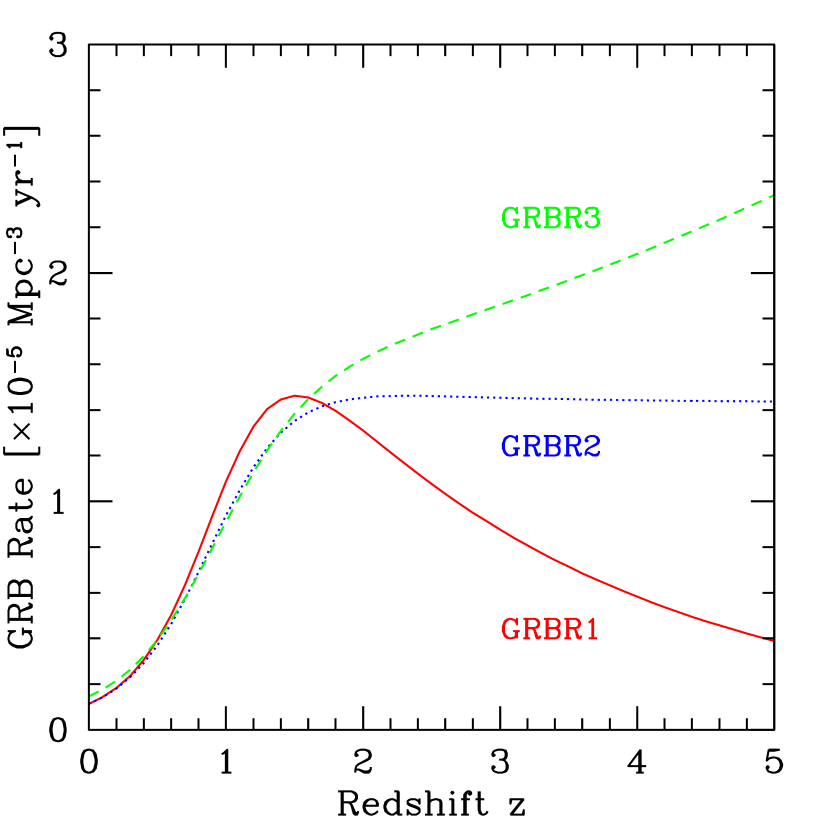
FIG. 1.: The cosmic GRB formation history. The solid, dotted and dashed curves show the rate of GRB formation per unit comoving volume as function of redshift for the models GRBR1, GRBR2, and GRBR3, respectively. $\Lambda$-dominated cosmology ($\Omega_{M}$=0.3, $\Omega_{\Lambda}$=0.7) is adopted. The Hubble constant is taken to be 70 km s^-1 Mpc^-1. The probability that one collapsar generates a GRB ($f$) is set to be 0.1.

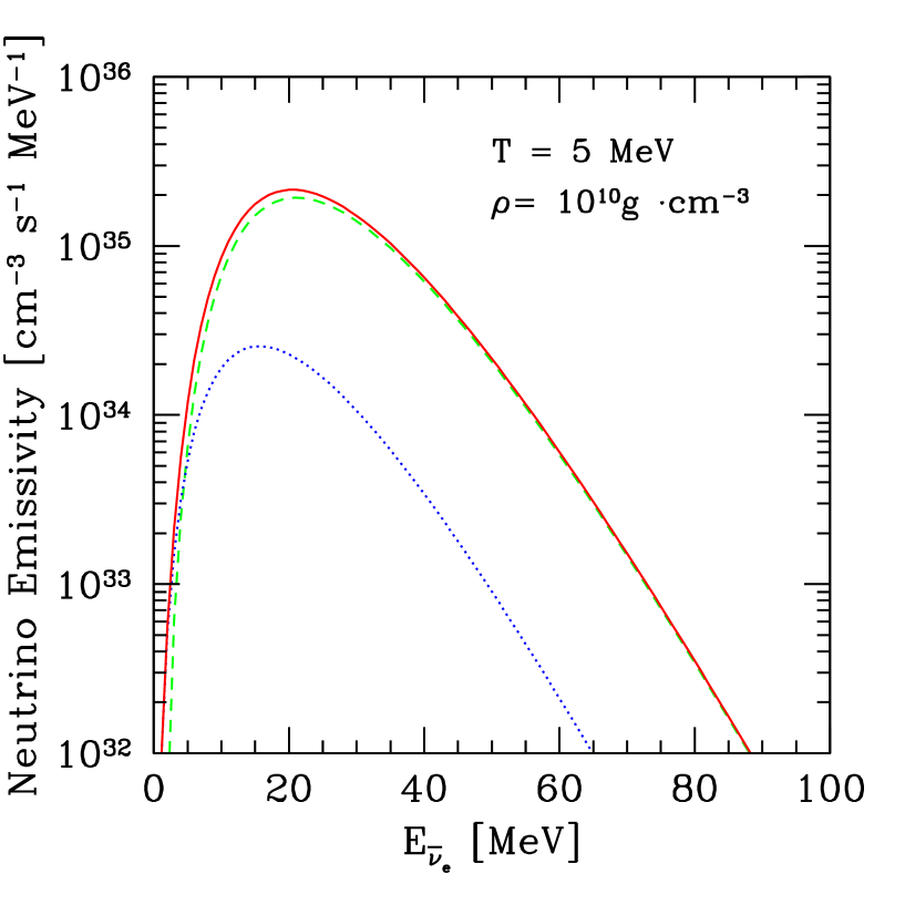
FIG. 2.: Emissivity of ${\overline{\nu}}_{e}$. Here we adopt $T$ = 5 MeV and $\rho=10^{10}{\rm g}\cdot{\rm cm}^{-3}$. Solid line represents the total emissivity of ${\overline{\nu}}_{e}$. Dashed (dotted) line is the contribution from $n+e^{+}\rightarrow p+{\overline{\nu}}_{e}$ ($e^{+}+e^{-}\rightarrow\nu_{e}+{\overline{\nu}}_{e}$).

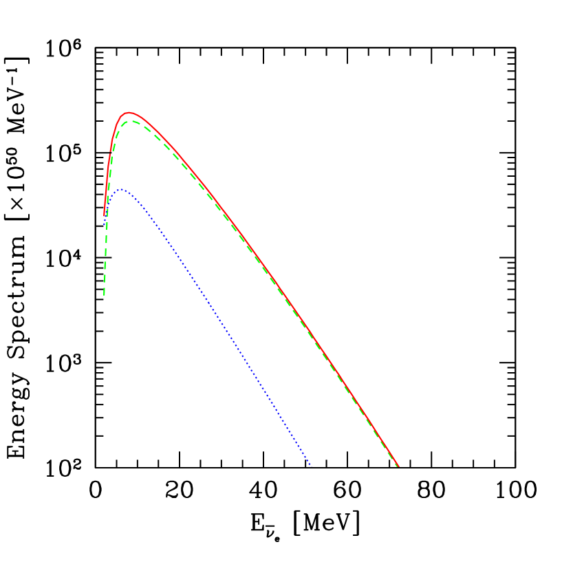
FIG. 3.: Energy spectrums of ${\overline{\nu}}_{e}$ from a collapsar. Solid line represents the total energy spectrum. Dashed (dotted) line is the contribution from $n+e^{+}\rightarrow p+{\overline{\nu}}_{e}$ ($e^{+}+e^{-}\rightarrow\nu_{e}+{\overline{\nu}}_{e}$). The total accreting mass, the initial mass, and the mass-accretion rate are set to be 30$M_{\odot}$, 3$M_{\odot}$, and 0.1$M_{\odot}$ $s^{-1}$, respectively.

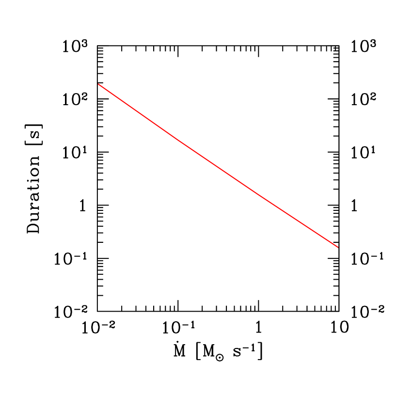
FIG. 4.: Duration of the neutrino emission from a collapsar as function of the mass-accretion rate. The total accreting mass and the initial mass are set to be 30$M_{\odot}$, 3$M_{\odot}$, respectively.

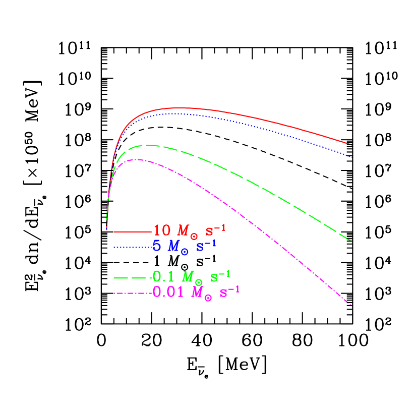
FIG. 5.: Dependence of the energy spectrum of anti-electron neutrino on the mass-accretion rate ($\dot{M}$). Solid line, dotted line, short-dashed line, long-dashed line, and dot-short-dashed line correspond to $\dot{M}$ = 10$M_{\odot}$ s^-1, 5$M_{\odot}$ s^-1, 1$M_{\odot}$ s^-1, 0.1$M_{\odot}$ s^-1 and 0.01$M_{\odot}$ s^-1, respectively.

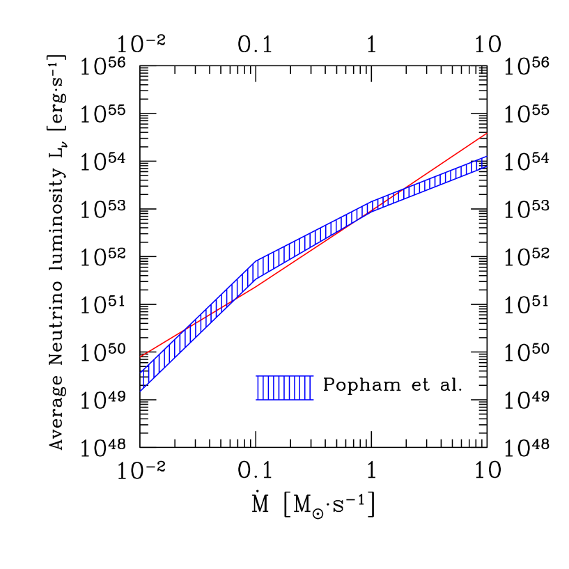
FIG. 6.: Average neutrino luminosity as a function of $\dot{M}$. We also show the result of Popham et al. (1999) for comparison.

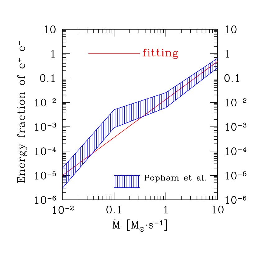
FIG. 7.: Efficiency of $\nu_{e}{\overline{\nu}}_{e}$ pair annihilations as a function of the mass-accretion rate. For comparison, we also show the result of Popham et al. (1999) as a shaded region.

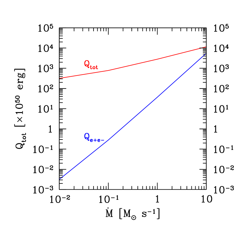
FIG. 8.: Total energy of emitted neutrinos ($Q_{\rm tot}$) and total deposited energy ($Q_{e+e-}$) in units of erg as a function of the mass-accretion rate.

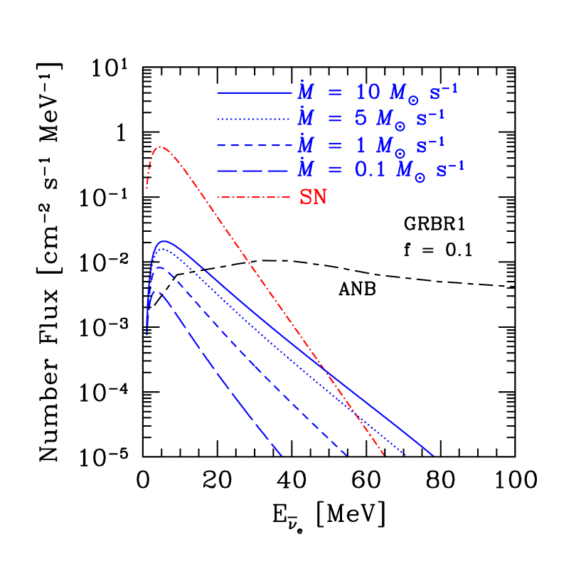
FIG. 9.: Differential number flux of GRB neutrino background [cm^-2 s^-1 MeV^-1]. Solid line, dotted line, short-dashed line, and long-dashed line correspond to $\dot{M}$ = 10$M_{\odot}$ s^-1, 5$M_{\odot}$ s^-1, 1$M_{\odot}$ s^-1, and 0.1$M_{\odot}$ s^-1, respectively. The case of SN neutrino background and atmospheric neutrino background (ANB) are shown in dot-short-dashed line and long-short-dashed line for comparison.

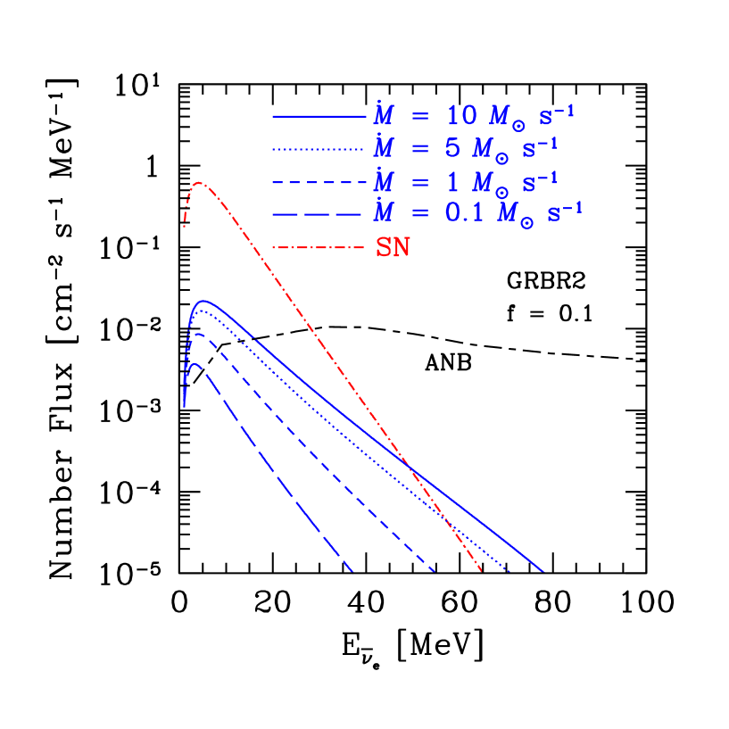
FIG. 10.: Same as Fig.9 but GRBR2 is used.

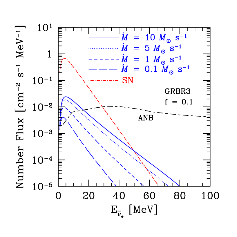
FIG. 11.: Same as Fig.9 but GRBR3 is used.

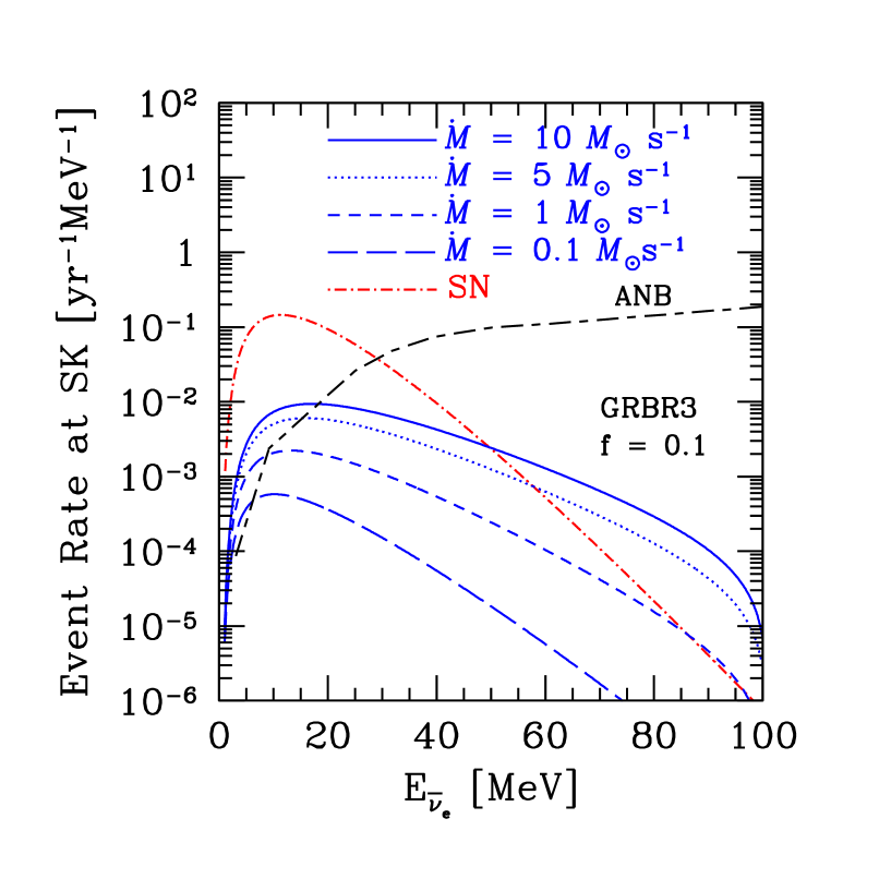
FIG. 12.: Event rate of GRB neutrino background [yr^-1 MeV^-1] at Super-Kamiokande. Solid line, dotted line, short-dashed line, and long-dashed line correspond to $\dot{M}$ = 10$M_{\odot}$ s^-1, 5$M_{\odot}$ s^-1, 1$M_{\odot}$ s^-1, and 0.1$M_{\odot}$ s^-1, respectively. Event rate of SN neutrino background and atmospheric neutrino background (ANB) are shown in dot-short-dashed line and long-short-dashed line for comparison.

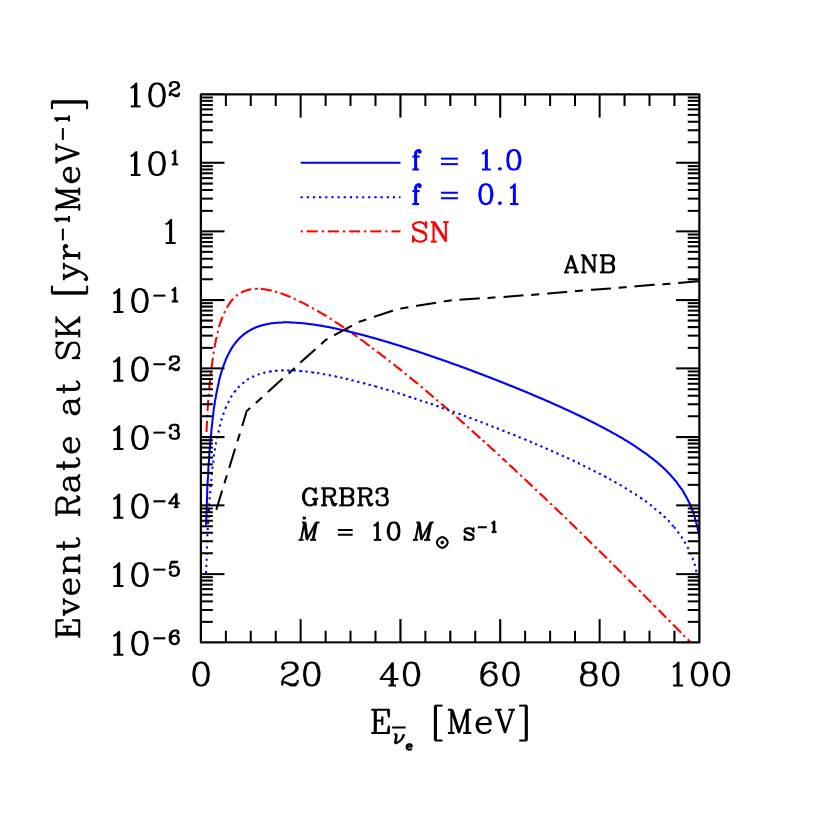
FIG. 13.: Dependence of the event rates on the probability $f$ that one collapsar generates a GRB. Solid line and dotted line correspond to the case $f=1.0$ and $f=0.1$, respectively. We adopt the case of $\dot{M}=10M_{\odot}{\rm s}^{-1}$

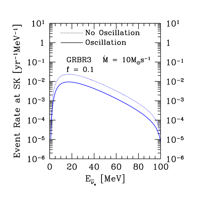
FIG. 14.: Event rate at SK for the model of $\dot{M}=10M_{\odot}$. Solid lines represent the case in which the effects of neutrino oscillation are taken into consideration. Dotted lines represent the case of no oscillation.

TABLE I.: Event Rate (yr^-1) and Statistical Error of ANB at SK/TITAND

	$N$ (yr-1)	$\sqrt{N\rm(yr^{-1})}$
$E_{\bar{\nu}_{e}}$ = (50 – 60)MeV	1.0/1.0$\times 10^{2}$	1.0/1.0$\times 10^{1}$
$E_{\bar{\nu}_{e}}\geq$ 50MeV	2.6/2.6$\times 10^{2}$	1.6/1.6$\times 10^{1}$

TABLE II.: Event Rate (yr^-1) of Signals at SK/TITAND

$\dot{M}$ ($M_{\odot}$s-1)	$f$	Oscillation	GRBR	$E_{\bar{\nu}_{e}}=$(50 – 60)MeV	$E_{\bar{\nu}_{e}}\geq$50MeV
10	0.1	Yes	3	9.1$\times 10^{-3}$/9.1$\times 10^{-1}$	1.7$\times 10^{-2}$/1.7
10	0.5	Yes	3	4.5$\times 10^{-2}$/4.5	8.6$\times 10^{-2}$/8.6
10	1.0	Yes	3	9.1$\times 10^{-2}$/9.1	1.7$\times 10^{-1}$/1.7$\times 10^{1}$
10	0.1	No	3	1.8$\times 10^{-2}$/1.8	3.4$\times 10^{-2}$/3.4
10	0.5	No	3	9.0$\times 10^{-2}$/9.0	1.7$\times 10^{-1}$/1.7$\times 10^{1}$
10	1.0	No	3	1.8$\times 10^{-1}$/1.8$\times 10^{1}$	3.4$\times 10^{-1}$/3.4$\times 10^{1}$
5	0.1	Yes	3	4.6$\times 10^{-3}$/4.6$\times 10^{-1}$	8.3$\times 10^{-3}$/8.3$\times 10^{-1}$
5	0.5	Yes	3	2.2$\times 10^{-2}$/2.2	4.2$\times 10^{-2}$/4.2
5	1.0	Yes	3	4.6$\times 10^{-2}$/4.6	8.3$\times 10^{-2}$/8.3
5	0.1	No	3	9.1$\times 10^{-3}$/9.1$\times 10^{-1}$	1.7$\times 10^{-2}$/1.7
5	0.5	No	3	4.6$\times 10^{-2}$/4.6	8.3$\times 10^{-2}$/8.3
5	1.0	No	3	9.1$\times 10^{-2}$/9.2	1.7$\times 10^{-1}$/1.7$\times 10^{1}$
1	0.1	Yes	3	8.3$\times 10^{-4}$/8.3$\times 10^{-2}$	1.4$\times 10^{-3}$/1.4$\times 10^{-1}$
1	0.5	Yes	3	4.2$\times 10^{-3}$/4.2$\times 10^{-1}$	6.9$\times 10^{-3}$/6.9$\times 10^{-1}$
1	1.0	Yes	3	8.3$\times 10^{-3}$/8.3$\times 10^{-1}$	1.4$\times 10^{-2}$/1.4
1	0.1	No	3	1.7$\times 10^{-3}$/1.7$\times 10^{-1}$	2.7$\times 10^{-3}$/2.7$\times 10^{-1}$
1	0.5	No	3	8.3$\times 10^{-3}$/8.3$\times 10^{-1}$	1.4$\times 10^{-2}$/1.4
1	1.0	No	3	1.7$\times 10^{-2}$/1.7	2.7$\times 10^{-2}$/2.7

TABLE III.: Time (yr) Required to Detect the Signals at SK/TITAND

$\dot{M}$ ($M_{\odot}$s-1)	$f$	Oscillation	GRBR	$E_{\bar{\nu}_{e}}=$(50 – 60)MeV	$E_{\bar{\nu}_{e}}\geq$50MeV
10	0.1	Yes	3	1.3$\times 10^{4}$/1.3$\times 10^{2}$	2.3$\times 10^{4}$/2.3$\times 10^{2}$
10	0.5	Yes	3	5.1$\times 10^{2}$/5.1	9.3$\times 10^{2}$/9.3
10	1.0	Yes	3	1.3$\times 10^{2}$/1.3	2.3$\times 10^{2}$/2.3
10	0.1	No	3	3.1$\times 10^{3}$/3.1$\times 10^{1}$	5.8$\times 10^{3}$/5.8$\times 10^{1}$
10	0.5	No	3	1.3$\times 10^{2}$/1.3	2.3$\times 10^{2}$/2.3
10	1.0	No	3	3.2$\times 10^{1}$/3.2$\times 10^{-1}$	5.8$\times 10^{1}$/5.8$\times 10^{-1}$
5	0.1	Yes	3	5.0$\times 10^{4}$/5.0$\times 10^{2}$	9.9$\times 10^{4}$/9.9$\times 10^{2}$
5	0.5	Yes	3	2.0$\times 10^{3}$/2.0$\times 10^{1}$	4.0$\times 10^{3}$/4.0$\times 10^{1}$
5	1.0	Yes	3	5.0$\times 10^{2}$/5.0	9.9$\times 10^{2}$/9.9
5	0.1	No	3	1.3$\times 10^{4}$/1.3$\times 10^{2}$	2.5$\times 10^{4}$/2.5$\times 10^{2}$
5	0.5	No	3	5.0$\times 10^{2}$/5.0	9.9$\times 10^{2}$/9.9
5	1.0	No	3	1.3$\times 10^{2}$/1.3	2.5$\times 10^{2}$/2.5
1	0.1	Yes	3	1.5$\times 10^{6}$/1.5$\times 10^{4}$	3.7$\times 10^{6}$/3.7$\times 10^{4}$
1	0.5	Yes	3	6.0$\times 10^{4}$/6.0$\times 10^{2}$	1.5$\times 10^{5}$/1.5$\times 10^{3}$
1	1.0	Yes	3	1.5$\times 10^{4}$/1.5$\times 10^{2}$	3.7$\times 10^{4}$/3.7$\times 10^{2}$
1	0.1	No	3	3.8$\times 10^{5}$/3.8$\times 10^{3}$	9.2$\times 10^{5}$/9.2$\times 10^{3}$
1	0.5	No	3	1.5$\times 10^{4}$/1.5$\times 10^{2}$	3.7$\times 10^{4}$/3.7$\times 10^{2}$
1	1.0	No	3	3.8$\times 10^{3}$/3.8$\times 10^{1}$	9.2$\times 10^{3}$/9.1$\times 10^{1}$