Why Do Disks Form Jets?

Abstract

It is argued that jet modelers have given insufficient study to the natural magneto-static configurations of field wound up in the presence of a confining general pressure. Such fields form towers whose height grows with each twist at a velocity comparable to the circular velocity of the accretion disk that turns them. A discussion of the generation of such towers is preceded by a brief history of the idea that quasars, active galaxies, and galactic nuclei contain giant black holes with accretion disks.

Institute of Astronomy, The Observatories, Madingley Road, Cambridge, CB3 0HA, UK & Clare College, Cambridge, UK

1. Introduction and History

Before a child learns to run, it must learn to walk. Before it learns to walk, it must learn to stand. I believe that those of us studying jets and winds from rotating objects have been guilty of attempting to run before we have understood how to stand.

Here I give an account of the natural sequence of static magnetic structures that are obtained by the continued twisting of a local poloidal magnetic field by an accretion disk. My contention is that had we understood such structures long ago, then we would have considered the jets seen in nature to be an obvious consequence of the twisting of the field by an accretion disk in the presence of an external pressure. If we imagine the accretion disk as turning all the time, then we have to consider a sequence of equilibrium models in which the total twist angles increase linearly with time. This sequence of models gives towers whose height increases with time at a velocity of the order of the maximum rotation velocity in the disk.

Although I gave the first account of these growing towers in Lynden-Bell (1996), the magnetohydrodynamic wind modelers were already much more sophisticated and it is only recently that Li et al. (2001) decided that such an elementary model may give a fundamental clue to what is really going on. Their numerical method was not capable of exploring such models beyond the first two twists. While these are highly indicative of what happens, the many-twist picture is best understood from the somewhat more realistic version of my 1996 paper given here. The essentials of the process can be understood without any detailed mathematics and with only the minimal knowledge of magnetohydrodynamics contained in Alfvén’s theorem that magnetic flux moves with the fluid. Those primarily interested in the magnetic towers model of jets may be advised to move direct to §2 unless they have an interest in the history of the subject.

I was originally invited to give an account of black holes in galactic nuclei, a subject I had some hand in starting, but by now there are those far better qualified to discuss the recent exciting data and David Merritt has given a magnificent critical account here. My counter-suggestion of giving some account of the history of black holes in galactic nuclei followed by my recent work on jets was accepted, so I shall now turn to history.

Since the Isaac Newton Group is running this conference there is no better starting point than Newton’s first Query in his Opticks of 1704:

And do not Bodies act upon Light at a distance and, by their action, bend its Rays, and is not this action (caeteris paribus) strongest at the least distance?

In 1784, moving on by 80 years we get to the Reverend John Michell’s great paper that not only predicted giant black holes but told us how massive they would be and how they would be found. Michell was a remarkable scientist, one of the founders of the geology of the UK through his early stratigraphy. He was the first to suggest that earthquakes traveled as waves. Other achievements of his were the experimental demonstration of an inverse square law between magnetic poles, the determination of the first luminosity function (using the Pleiades), the statistical demonstration that binary stars were gravitationally associated, a method for measuring the motion of the Sun through nearby stars and the invention of the apparatus for measuring $G$, the gravitational constant. This was perfected and first successfully used after his death by his great friend Henry Cavendish. Erasmus Darwin, grandfather of Charles, was among Michell’s more prominent students at Cambridge. Michell in a paper in the Philosophical Transactions of the Royal Society for 1784 argued that bodies of greater than 500 times the diameter of the Sun and not of lesser density would so attract the light that it could not escape, rendering such great masses invisible to our senses. Nevertheless, he thought, they might be detected through observations of small satellites circling about them. It is interesting that $(500)^{3}\ M_{\odot}=1.25\times 10^{8}\ M_{\odot}$ (Mitchell 1784), while the first definitive observation of a giant black hole by Miyoshi et al. (1995) used material circling around it to determine its mass—$3.6\times 10^{7}\ M_{\odot}$. Such predictions more than 200 years in advance of their time are extremely rare!

We know that Michell’s idea traveled to the French academy not only by the customary exchange of journals but also it was discussed in an exchange of letters between the botanist Sir Joseph Banks, President of the Royal Society, and Benjamin Franklin, who was then (1783) US Ambassador in Paris. Two years after Michell died, Laplace described the idea of dark stars (without attribution) in his Système du Mond Laplace (1795), using exactly Michell’s argument translated into French, but in 1802 Young published his two-slit experiment demonstrating the wave nature of light (Young 1802). This put in doubt Michell’s arguments, based on the corpuscular theory of light, so Laplace deleted the passage on dark stars from the second edition of his book.

The well known historian of science Agnes Clarke, writing an account of Michell’s life and work for The Dictionary of National Biography (Clarke 1917), ended her list of Michell’s scientific achievements with the words

But [he] speculated fruitlessly on a supposed retardation of light through the attraction of its corpuscles by the emitting masses.

This almost certainly reflects the received wisdom of the British astronomers of the time.

Returning to the 1780s, Sir William Herschel (1786) remarked upon the bright nuclei of the galaxies we now know as NGC 4151 and NGC 1068 and in 1850 Lord Rosse, using the giant telescope he had developed at Birr Castle, discovered spiral structure in M51 and other galaxies (Rosse 1850).

Coming to the 20th century, Vesto Slipher (1917), taking long time-exposed spectra photographically with a 36 inch telescope, discovered broad emission lines in these galaxies. They were so broad that he decided some non-Doppler broadening mechanism must be involved. It is seldom pointed out that most of the early redshifts of galaxies are due to Slipher’s work. He did not claim that the Universe was expanding because he thought similar work in the southern hemisphere might find almost nothing but blueshifts. However, his work was used by Eddington (1922) in his book on general relativity.

In 1918 Curtis photographed the jet at the centre of M87 (Curtis 1918). Even the emission mechanism remained a mystery until Baade showed it to be polarized synchrotron emission in 1952. Synchrotron emission was first worked out by Schott (1912) but it was not recognized as an emission mechanism in astronomy until the 1950s.

The major postwar development of astronomy came out of British developments in RADAR. In the years 1955–1975 Sir Martin Ryle led his Cambridge team to a series of remarkable discoveries which impacted almost all parts of the subject from stellar death to cosmology (Ryle 1968). Thus the third Cambridge Catalogue of radio sources and their 3C numbers became deeply embedded in the subject. Ryle and Hewish together developed aperture synthesis as a tool. In this they were helped not a little by a secret weapon. David Wheeler in Cambridge had developed a program for inverting Fourier transforms which was many times faster than others then in use. When some ten years later the method was rediscovered and published by Cooley and Tukey it rightly became famous.

Henry Palmer of Jodrell Bank led a team that developed linked radio telescopes over considerable distances and showed that a small fraction of the 3C sources contained small-angular-diameter sources down to a few arcseconds. Hazard realized that an accurate position for one of these could be obtained from a lunar occultation that would take place in Australia (Hazard, Mackay, & Shimmins 1963). Such positions were vital for the identification programs which Schmidt and Sandage had started at the Mt Wilson and Palomar Observatories. The first quasar spectrum to be taken was that of 3C48 by Greenstein. This showed emission lines at wavelengths that defied identification. Later that year (1963) Hazard sent Schmidt the lunar occultation position of 3C273. Luckily this showed two lines whose wavelength ratio exactly matched those of the hydrogen spectrum at the amazing redshift of $z=0.158$, quite unheard of for a 12^th magnitude object.

Schmidt’s (1963) identification was soon confirmed by Oke’s (1963) detection of a third hydrogen line in the infrared. With the clues provided by 3C273, Greenstein’s spectrum of 3C48 was then interpreted as having a redshift of $z=0.367$. Soon afterwards, Greenstein & Schmidt (1964) collaborated on a paper that demonstrated that the high redshifts of the quasars could not be of gravitational origin. The emission lines needed a large volume for their formation and in a strong gravity field this would involve much greater line broadening than the emission lines showed. Hoyle and Fowler tried to get out of this by putting the source of emission at the centre of a very massive large stellar system which provided the potential but such a contrived model acquired few backers.

Early attempts to find cluster galaxies associated with quasars failed and this let to the idea that quasars were not associated with galaxies at all. Novikov (1964) and Ne’eman (1965) independently put forward the idea that they were white holes—time-delayed pieces of the Big Bang. It was Salpeter who first considered a massive object ploughing through a galaxy and accreting interstellar gas. Assuming that the material gradually percolated down to the last stable circular orbit, he gave the 5.7% efficiency of turning mass into energy. The properties of the orbits in Schwarzschild’s metric had indeed been known to relativists for some years, Zel’dovich among them.

Three papers laid the foundation of the thin accretion disk model now widely used

• Salpeter, E.E. 1964, ‘Accretion of interstellar matter by massive objects’, ApJ, 140, 796

• Lynden-Bell, D. 1969, ‘Galactic nuclei as collapsed old quasars’, Nat, 223, 690

• Bardeen, J. 1970, ‘Kerr metric black holes’, Nat, 226, 64

G. Burbidge (1959) gave minimum energy estimates of order $10^{61}$ erg for a number of radio sources and rightly emphasized that this was a very large number, while well before quasars Ambartsumian had emphasized the extraordinary behavior and high energy emissions from galactic nuclei (Ambartsumian & Shakbuzian 1958).

The main points of my 1969 paper were:

1. $10^{61}$ erg weigh $\hbox{$\,{}^{1}\!/_{2}$}10^{7}\ M_{\odot}$. If these ergs arise from nuclear fusion then $10^{9}\ M_{\odot}$ must be involved. But quasars vary in as little as 10 hours and $G(10^{9}\ M_{\odot})^{2}/(10\ {\rm light\ hour})\gg 10^{61}\ {\rm erg}$. The assumption that the energy is nuclear therefore leads to an even greater gravitational binding energy which must have been lost. Thus the assumption is wrong.

   Hence most of the power of quasars is gravitational in origin and masses $\sim 10^{8}\ M_{\odot}$ suffice. But there are no dead states like white dwarfs for such masses, except black holes. If emission is not 100% efficient remnants must remain.

2. I next considered the number of dead QSOs—based on Sandage’s (1965) estimates of them—and obtained

   $$\left(\begin{array}[]{c}{\rm number\ of\ clusters}\\ {\rm of\ galaxies}\end{array}\right)<\left(\begin{array}[]{c}{\rm number\ of}\\ {\rm dead\ quasars}\end{array}\right)<\left(\begin{array}[]{c}{\rm number\ of}\\ {\rm galaxies}\end{array}\right).$$

3. How do we hide dead quasars of $\sim 10^{8}\ M_{\odot}$ when they still gravitate? They are likely to be in dense places and to surround themselves with stars. Thus the obvious place to find them is in galactic nuclei.

4. What should dead quasars look like? Taking them to accrete via a friction caused by magnetic torques, I derived a temperature distribution $T(r)\propto r^{-3/4}$ and adding many such rings of black hole body emission gave me

   $$S_{\nu}\propto F_{M}^{2/3}\nu^{1/3}\exp-(h\nu/kT_{\rm max}),$$

   where $F_{M}$ is the rest-mass flux down the hole.

5. Observational predictions were that most large galaxies should have nuclei with high M/L when inactive. In calling the paper ‘Galactic nuclei as collapsed old quasars’, I was raising the question “Are galactic nuclei just stars gathered around such black hole remnants of quasars?”

The masses of the black holes estimated in 1969, mainly from Merle Walker’s observations using the Lallmand image-tube, are compared with modern values in Figure 1. It is clear that these old estimates are mostly too high by a factor of order ten because no allowance was made for the mass of stars in the nuclei.

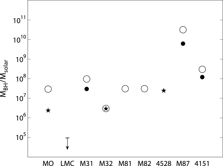
Figure 1.: My 1969 estimates of Black Hole masses $\circ$, compared with modern determinations - $\star$ good, and $\bullet$ less definitive.

At the time, most working astronomers were highly sceptical of the whole picture, but Maarten Schmidt volunteered that it seemed the best theory available to explain the amazing phenomena.

It was clear that as a black hole accreted from the last stable orbit it would accrete angular momentum as well as mass. It thus became important to work out accretion disks with Kerr holes. I had a friendly competition with Jim Bardeen to do this and his knowledge of general relativity gave him a head start which he easily kept. His short but beautiful paper (Bardeen 1970) shows how a Schwarzschild hole evolves into an extreme Kerr hole as it accretes. Some of this is covered in my Vatican review (Lynden-Bell 1971a) and radio observations of the Galactic Centre were made then (Ekers & Lynden-Bell 1971).

In 1971 I reviewed the data on the Galactic Centre with Martin Rees (Lynden-Bell & Rees 1971) and some further details of Kerr disks and vortices were given later (Lynden-Bell 1978, 1986), but by then the field had become overpopulated.

A maximum likelihood method for determining luminosity functions was developed and applied to quasars and miniquasars (Lynden-Bell 1971b,c).

2. Jets from Accretion Disks

Jets were not generally acknowledged to feed radio lobes before Rees’s (1971) theory. Jets are seen in nature associated with radio galaxies (M87, Cygnus A; Hargrave & Ryle 1974), quasars (3C273, 3C47), young stars (Beckwith et al. 1990; Bouvier 1990) Herbig–Haro objects (Bontemps et al. 1996; Burrows et al. 1996), dying stars (SS 433), and micro-quasars (Mirabel & Rodriguez 1999).

One common feature is that the jet velocities are of the order of the circular velocity that would balance gravity at the central object’s surface.

Theoretical models of jets fall into three classes:

1. Hydrodynamic models collimated by Laval nozzles (Blandford & Rees 1974), or by vortices around black holes (Lynden-Bell 1978), or by self-similar thick disks (Gilham 1981; Narayan & Yi 1995; Narayan, Barret, & McClintock 1997).

2. Wind models in some way collimated by the local magnetic field of the rotating source (Mestel 1968; Blandford & Znajek 1977; Sakurai 1985, 1987; Heyvaerts & Norman 1989; Appl & Camenzind 1993; Lery et al. 1998; Lynden-Bell 1996; Okamoto 1997, 1999; Li et al. 2001).

3. Models collimated by a large-scale pre-existing magnetic field (Lovelace 1976; Blandford & Payne 1982; Shibata & Uchida 1985, 1986; Begelman & Li 1994; Bell & Lucek 1995; Lucek & Bell 1996; Ouyed & Pudritz 1997; Ouyed, Pudritz, & Stone 1997; Vlahakis & Tsinganos 1998).

Models in class 3 certainly work but their collimation is no surprise since the large-scale magnetic field provides collimation at great distances. A body of plasma initially fired across the field at some angle $\theta$ to it would have its transverse motion resisted by the field (a high conducting background medium being assumed) but its $\cos\theta$ motion along the field would continue. Eventually it would be collimated to move along the field. Thus, to some degree, all such models provide collimation by fiat in the boundary conditions. They cannot provide collimation in dying stars or bodies such as SS 433 in which the jets precess (Margon 1984).

The prevalence of electromagnetic phenomena associated with all jets and the acceleration of some particles to very high energies with relativistic motions strengthen the idea that the jets themselves may be an electromagnetic phenomenon and even the early advocates of purely hydrodynamic jets have more recently turned to magnetohydrodynamic models. This is partly because of the difficulty of getting sufficiently high speeds but also because it was difficult to obtain the extremely narrow jets like those seen in Cygnus A and HH 30.

Here we shall therefore concentrate on the models in class 2, in which the jets are collimated not by external fields but by fields associated with the objects themselves. Work in this area began from consideration of stellar winds and the angular momentum that they transported thereby braking stellar rotation, but it took on a new life in the discussion of pulsars. Following Sakurai’s early work there has been much discussion of asymptotic collimation of such winds, however the whole subject has been put in a well ordered form in Mestel’s (1999) book so the interested reader may find it there. I gave a brief review of the still active controversies in my introduction to the Royal Society’s meeting on Magnetic Activity in Stars, Disks and Quasars (Lynden-Bell et al. 2000).

As stated in the introduction, we shall now turn to my growing-towers picture (Lynden-Bell 1996) based on motion through a sequence of static structures that inevitably occur when a poloidal magnetic field is progressively twisted.

2.1. Magneto-Static Theorems and Rough Estimates

We consider a magnetic field anchored on the plane $z=0$ and confined by an ambient external pressure $p_{0}$ due to an ionized medium. Where there is field there is no gas pressure and except at the surface of the volume $V$ occupied by field (and $z=0$) the field configuration is force free. The total energy of the configuration may be written

$$W=W_{R}+W_{\phi}+W_{z}+W_{p}=\frac{1}{8\pi}\int\left(B^{2}_{R}+B^{2}_{\phi}+B^{2}_{z}\right)dV+p_{0}V.$$

We have taken cylindrical polar components of the field for our later convenience but the theorems proved are not confined to fields of any particular symmetry. Now the field wiggles its way to the minimum energy configuration subject to the constraints imposed by the boundary conditions on the disk. These define the vertical field component $B_{z}$ on $z=0$ and the twist angles of each field line which are most easily conceived for the axially symmetric case in which they are measured as twists about the axis. It may be shown that the force free equations follow from minimizing the energy subject to the constraints.

Theorem 1

For any finite magneto-static configuration anchored on z = 0 then on any cut z = constant

$$w_{R}+w_{\phi}=w_{z}+w_{p},$$

where ${\rm w}_{{\rm R},\phi,{\rm z}}$ = $[{\it 1/}({{\it 8}\pi})]\int{\rm B}^{2}_{{\rm R},\phi,{\rm z}}{\rm dA},\ {\rm w_{p}}={\rm p_{0}A}$ and A is the area of the volume V intersected by the cut.

Notice that the capital W are related to the small w by integration over z.

Proof  Consider the slice between the cut at $z$ and one at $z+dz$. Lift the whole field configuration above $z+dz$ rigidly by an amount $(\lambda-1)dz$, expand the slice to thickness $\lambda dz$ and leave the configuration below $z$ unchanged (see Figure 2). In the vertical expansion of the slice flux conservation gives

$$B_{R}\rightarrow B_{R}/\lambda\ ,\ \ B_{\phi}\rightarrow B_{\phi}/\lambda\ ,\ \ B_{z}\rightarrow B_{z}\ ,\ \ dAdz\rightarrow\lambda dAdz.$$

Thus in terms of the old fields and old $w$

$$\Delta W=\left[(w_{R}+w_{\phi})\ (\lambda^{-1}-1)+(w_{z}+w_{p})\ (\lambda-1)\right]dz.$$

Now the original situation must be a minimum energy one, so $\partial(\Delta W)/\partial\lambda$ must be zero at $\lambda=1$. This condition yields at once $w_{R}+w_{\phi}=w_{z}+w_{p}$ (QED).

Theorem 2

For any finite magneto-static configuration anchored on z = 0

$$W_{z}=W_{p}+\hbox{$\,{}^{1}\!/_{2}$}W_{0},$$

where ${\rm W_{\it 0}}$ = ${\rm[{\it 1/}({\it 4\pi})]\int B_{z}B_{R}RdA}$ evaluated on z = 0.

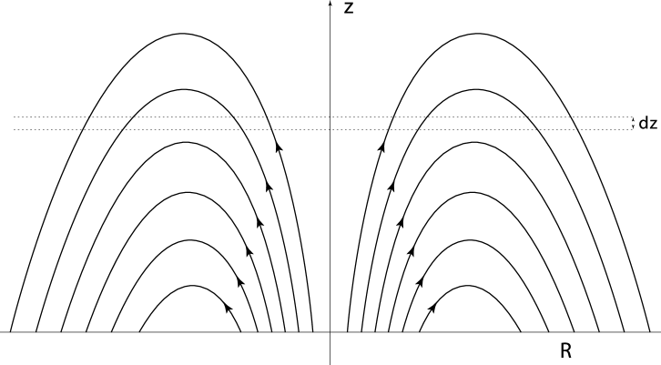
Figure 2.: A slice of a force-free field structure. The twists about the axis are not shown. The theorem is true without assumptions of axial symmetry.

Proof  Consider a lateral expansion of the volume $V$ occupied by field such that $R\rightarrow\mu R,\ z\rightarrow z$. Conservation of flux across elementary areas $Rd\phi dz$, etc., gives $B_{R}\rightarrow B_{R}/\mu,\ B_{\phi}\rightarrow B_{\phi}/\mu,\ B_{z}\rightarrow B_{z}/\mu^{2},\ dA\rightarrow\mu^{2}dA$

$$\Delta W=W_{z}(\mu^{-2}-1)+W_{p}(\mu^{2}-1).$$

Now we must take care because, unlike our former transformation, this one moves the anchored foot-points on $z=0$. Luckily the principle of virtual work comes to our aid. We have to add to $\Delta W$ the work done in infinitesimal movement $\delta\mu R$ of the foot points by the forces of constraint, viz. $B_{R}B_{z}dA/(4\pi)$, so

$$\left[\frac{\partial\Delta W}{\partial\mu}\right]_{\mu=1}+\frac{1}{4\pi}\int_{z=0}B_{R}B_{z}RdA=0.$$

Thus we obtain

$$W_{z}=W_{p}+\hbox{$\,{}^{1}\!/_{2}$}W_{0}$$

(QED). To those who believe that the pinch effect needs no external pressure it comes as a surprise that $8\pi W_{\phi}=\int B^{2}_{\phi}\mu^{-2}\mu^{2}dAdz$, which is independent of $\mu$. Thus there is no tendency for overall contractions in a purely toroidal field. It is perhaps of interest to minimize the energy of a toroidal flux $F$ contained between cylinders of radii $R_{1}$ and $R_{2}$ of height $Z$. One finds $B_{\phi}\propto{1}/{R}$:

$$W_{\phi}=\frac{1}{4}\frac{F^{2}_{\phi}Z^{-1}}{{\rm ln}(R_{2}/R_{1})}.$$

Thus if $R_{2}$ and $R_{1}$ are increased by the same factor there is no change in $W_{\phi}$, in agreement with what we found above, but if $R_{2}$ is fixed then $W_{\phi}$ decreases as $R_{1}$ is reduced giving rise to a pinch. In fact $B^{2}_{\phi}\propto{1}/{R^{2}}$ shows that the toroidal magnetic field acts as a pressure amplifier delivering on $R_{1}$ a pressure $(R_{2}/R_{1})^{2}$ times that exerted on $R_{2}$. The whole pinch effect is a pressure amplifier—without anything to push on outside it has nothing to amplify and indeed the field would expand outwards as well as inwards.

To orient ideas it is useful to make some very crude dimensional estimates. Suppose the typical radius out to which the field expands laterally is $R_{2}$ and we deal with an axially symmetrical field configuration which is wound up by the turning of the accretion disk. Let the field pass upward through the disk at small radii and return downward at larger radii and let the total upward poloidal flux be $F$. With each turn of the upward flux relative to the downward a toroidal flux equal to $R$ will be generated, so after $n$ turns the toroidal flux will be $nF$. If $Z$ is the total height of the configuration then the volume $V$ occupied by field will be $V=\pi R^{2}_{2}Z$ a typical value of $B_{\phi}$ will be $nF/(R_{2}Z)$, a typical value of $B_{R}$ will be $F/(\sqrt{2}\pi RZ)$, and a typical value of $B_{z}$ will be $2F/(\pi R^{2}_{2})$; the $\sqrt{2}$ in $B_{R}$ comes from the fact that the typical $\pi R$ for a radial field line is $2\pi(R^{2}_{2}/2)^{1/2}$, while the factor 2 in the $B_{z}$ comes from the fact that the flux goes both up and down.

Dividing (2) by $A/(8\pi)$ yields the interesting exact result

$${\Big{\langle}}B^{2}_{R}{\Big{\rangle}}+{\Big{\langle}}B^{2}_{\phi}{\Big{\rangle}}={\Big{\langle}}B^{2}_{z}{\Big{\rangle}}+8\pi p_{0},$$

where the averages are taken over any $z={\rm constant}$ plane. Putting in our rough estimates we get

$$\frac{F^{2}}{2\pi^{2}R^{2}_{2}Z^{2}}\left(1+2\pi^{2}n^{2}\right)=\frac{4F^{2}}{\pi^{2}R^{4}_{2}}+8\pi p_{0}.$$

Now consider the case of no bounding pressure. Then

$$\frac{Z^{2}}{R^{2}_{2}}=\frac{1}{8}\left(1+2\pi^{2}n^{2}\right),$$

so ${Z}/{R}\rightarrow({\pi}/{2})n$ for $n$ large, which appears to show that the collimation $Z/R$ increases with every turn $n$. On first finding this I was much encouraged and immediately turned to get a more exact model. When I solved it I was deeply disappointed because before the field has twisted by even one turn it relieves itself by expanding to infinity with an opening angle of $120\hbox{${}^{\circ}$}$—very far from the sort of collimation we seek. Figure 3 shows the field configurations for twist angles of $130\hbox{${}^{\circ}$}$ and $180\hbox{${}^{\circ}$}$. When $208\hbox{${}^{\circ}$}=2\pi/\sqrt{3}^{c}$ is reached the field is outwards along cones up to $60\hbox{${}^{\circ}$}$ to the equator. This disconnection at infinity is precisely what was predicted by some pretty theorems of J.J. Aly (1995) but, although it provides a beautiful illustration of these, it fails to give the accurate collimation we seek. However, those interested in galaxies with conical outflows should perhaps pay more attention to this magneto-static result described in detail in Lynden-Bell & Boily (1994). I was so disappointed in the result, which was initially found in 1979, that I laid the whole subject aside and only returned to it in 1994. It took two more years before I realised that victory might still be snatched from the jaws of defeat. Expression (6) failed to give collimation only because $n$ could not be made large without the field disconnecting at infinity. If a way could be found to prevent the field reaching out to infinity then perhaps $n$ could be made large after all. This led me to introduce the ambient pressure $p_{0}$ to confine the field. It then takes an infinite amount of work for the field to extend to infinity so this will not occur at finite twist angles. Let us now turn to equation (3) and insert our rough estimates. On dividing by $V/8\pi$ we find

$$\frac{4F^{2}}{\pi^{2}R^{4}_{2}}=8\pi p_{0}+2\sqrt{2}\frac{F^{2}}{\pi R^{2}_{2}Z^{2}},$$

where we have left the $B_{z}$ field on the disk at $B_{z0}$ since this is fixed but used our estimate of $B_{R}$ there too. Eliminating $p_{0}$ between (7) and (5) we find

$$\frac{Z^{2}}{R^{2}}=\frac{1}{16}\left(2\sqrt{2}+1+2\pi^{2}n^{2}\right),$$

so asymptotically

$$Z/R\rightarrow\frac{\pi}{2\sqrt{2}}n,$$

just a factor $\sqrt{2}$ less than our first wrong estimate without $p_{0}$. With $Z^{2}/R^{2}$ large the last term in (7) is negligible compared with the first, so $W_{0}$ may be neglected compared with $W_{z}$. Furthermore, with $n$ large $B_{R}$ becomes negligible compared with $B_{\phi}$. Thus highly wound configurations become tall towers. For such we have from (4) at each height

$${\Big{\langle}}B^{2}_{\phi}{\Big{\rangle}}={\Big{\langle}}B^{2}_{z}{\Big{\rangle}}+8\pi p_{0}.$$

Furthermore, we may consider local transformations that expand $R\rightarrow\mu(z)R$ where $\mu(z)$ is slowly varying but becomes one except in a region around some chosen height. Even after this transformation the fields will still have $B_{R}$ small so its square is negligible compared with $B^{2}_{z}$. From such transformations, which leave $W_{0}$ unchanged, we can deduce that at any great height (3) may be replaced by $w_{z}=w_{p}$, so on dividing by $A/8\pi$

$${\Big{\langle}}B^{2}_{z}{\Big{\rangle}}\approx 8\pi p_{0}.$$

Hence from (8) we have everywhere well above the base $z=0$

$$\hbox{$\,{}^{1}\!/_{2}$}{\Big{\langle}}B^{2}_{\phi}{\Big{\rangle}}={\Big{\langle}}B^{2}_{z}{\Big{\rangle}}=8\pi p_{0},$$

where the averages are taken over areas at constant $z$.

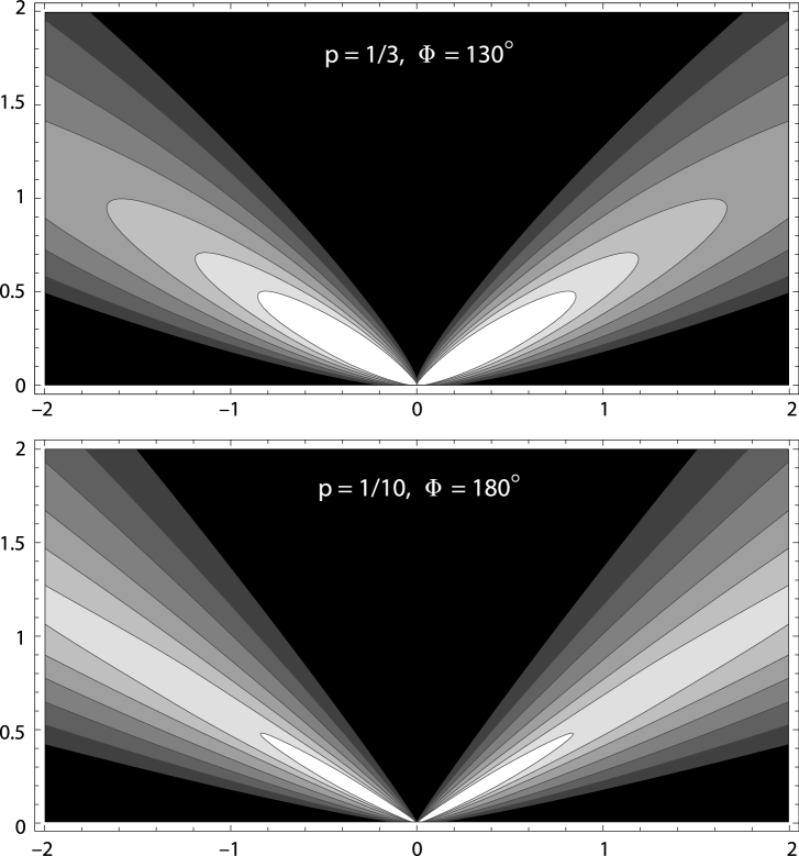
Figure 3.: Field lines splay out and reconnect at infinity after a twist of only $2\pi/\sqrt{3}$ rad $\approx 208\hbox{${}^{\circ}$}$ unless confined by an ambient pressure.

3. Better Estimates of the Field Structure

Consider the tube of force that intersects the accretion disk in the circle of radius $R_{1}$. Let the poloidal flux rising within this tube be $P$. Then we may label each field line by the value of $P$ and indeed $B_{z}=+[{1}/({2\pi R})]\partial P/\partial R$, $B_{R}={-[1}/({2\pi R})]{\partial P}/{\partial z}$. If this field line returns to the disk at some larger radius $R_{2}$ then there will be a differential twisting due to the fact that on the accretion disk $\Omega_{1}>\Omega_{2}$. We define $\Omega(P)=\Omega_{1}-\Omega_{2}$ so $\Omega(P)$ is the rate of twisting of the field line labeled $P$. Now suppose that at any given time $t$ when the twist angle will have accumulated to be $\Phi(P)=\Omega(P)t$ the field line labeled $P$ rises to a maximum height $Z(P)$. Then the total twist per unit height will be $\Phi(P)/Z(P)$. Now one turn (a twist of $2\pi$) will cause a toroidal flux between $P$ and $P+dP$ of just $dP$ so the toroidal flux per unit height between $P$ and $P+dP$ will be

$$\frac{\Phi(P)}{2\pi Z(P)}.$$

Now only those field lines with $P^{\prime}\leq P$ will reach to height $Z(P)$ so the total toroidal flux per unit height at $Z$ will be

$$\int^{R(P)}_{0}B_{\phi}dR=\int^{P}_{0}\frac{\Phi(P^{\prime})}{2\pi Z(P^{\prime})}dP^{\prime}$$

so

$$\bar{B}_{\phi}=\frac{1}{2\pi R(P)}\int^{P}_{0}\frac{\Phi(P^{\prime})}{Z(P^{\prime})}dP^{\prime},$$

where $P$ is the flux label of the line that just reaches height $Z(P)$ and no further. The radius of the area occupied by magnetic field at height $Z$ we call $R(Z(P))$, or $R(P)$ for short. This is not the radius at which the line labeled $P$ reaches height $Z$.

Now the flux $P$ is all the poloidal flux that crosses height $Z$ once on the way up and once on the way down, so the average $\langle|B_{z}|\rangle$ is $2P/\left\{\pi\left[R(P)\right]^{2}\right\}$. Since $B_{z}=(2\pi R)^{-1}\partial P/\partial R$ we may write

$${\Big{\langle}}B^{2}_{z}{\Big{\rangle}}=\int^{R(P)}_{0}\left(2\pi R\right)^{-1}\left(\partial P/\partial R\right)^{2}dR=\left(2P/\left\{\pi\left[R(P)\right]^{2}\right\}\right)^{2}I,$$

where $I$ is the dimensionless integral given by

$$I=\frac{\pi}{8}\int^{1}_{0}\left(\partial\tilde{P}/\partial\tilde{R}\right)^{2}\tilde{R}^{-1}d\tilde{R}$$

and

$$\tilde{P}=P^{\prime}(R^{\prime})/P,\ \tilde{R}=R^{\prime}/R(P).$$

By the theorem that the mean square is greater than or equal to the square of the mean modules $I\geq 1$.

Now in a self-similar distribution of field $I$ would be independent of $Z$ so we shall suppose that at heights well above the base at $z=0$, $I$ depends on $Z$ only weakly if at all. Using (13) for ${\Big{\langle}}B^{2}_{z}{\Big{\rangle}}$ in (10) we find

$$\pi\left[R(P)\right]^{2}=P\left[I/(2\pi p_{0})\right]^{1/2},$$

so neglecting the variation of $\log I$,

$$d\ln R(P)/d{\rm ln}P=1/2.$$

Now let ${\Big{\langle}}B^{2}_{\phi}{\Big{\rangle}}{\Big{/}}\bar{B}^{2}_{\phi}=J.$ Then from (10) and (12)

$$\int^{P}_{0}\frac{\Phi(P^{\prime})}{Z(P^{\prime})}dP^{\prime}=8\pi\left(\frac{\pi p_{0}}{J}\right)^{1/2}R(P).$$

Differentiating with respect to $P$ and using (17) and (16),

$$\Phi(P)/Z(P)=4\pi(\pi p_{0}/J)^{1/2}R(P)/P=(8I/J)^{1/2}/R(P),$$

where we have neglected the variation of $J$ with height. Hence

$$\frac{Z(P)}{R(P)}=\frac{\Phi(P)}{(8I/J)^{1/2}},$$

or, since $\Phi(P)=\Omega(P)t$,

$$Z(P)=(8I/J)^{1/2}\Omega(P)R(P)t,$$

so the maximum height of each field line grows linearly in time at a velocity related to the disk’s circular velocity, and the area occupied by the field at height $Z(P)$ is proportional to $P$ as given by (16).

To proceed further we need to determine $\Omega(P)$, which is one of the inputs of our model since it is determined by the distribution of the poloidal flux over the disk as well as the disk’s rotation.

We shall take our accretion disk to be Keplerian outside some radius $R_{0}$ so that the circular velocity

$$V=V_{0}(R_{0}/R_{1})^{1/2}\hskip 28.45274pt(R_{1}>R_{0})$$

however, such a law cannot continue down to $R_{1}=0$ as it would lead to infinite velocities. We shall therefore take circular velocities of the form

$$V=V_{0}{\Big{[}}1+\left(R_{1}/R_{0}\right)^{2}{\Big{]}}^{-1/4}.$$

My original accretion disk model of quasars (Lynden-Bell 1969) relied on shearing and reconnecting magnetic fields giving stresses to provide the torques which allowed the material to lose its angular momentum and be accreted. It gave magnetic fields $B\propto R^{-5/4}$, and more recent accretion disk models (e.g., Shakura & Sunyaev 1973, 1976; Tout & Pringle 1992), which rely on the less reliable $\alpha-$viscosity, give the same $R$ dependence for magnetic fields. However, again the field must reach some finite value as $R_{1}$ becomes small so we shall take on the disk $z=0$

$$B_{z}=B_{0}(1+(R_{1}/R_{0})^{2})^{-5/8}.$$

This gives a convenient flux function

$$P=F_{0}\frac{8}{3}\left\{\left[1+\left(R_{1}/R_{0}\right)^{2}\right]^{3/8}-1\right\}\hskip 28.45274pt{\rm for}\ P\geq F_{0}$$

where $F_{0}=\pi R^{2}_{0}B_{0}$. We shall assume there is a total poloidal flux $F$ so $P\leq F$. Eliminating $R_{1}/R_{0}$ we obtain

$$V=V_{0}\left[1+(3/8)P/F_{0}\right]^{-2/3}\hskip 28.45274pt({\rm for}\ P\leq F)$$

or writing $\Omega_{0}=V_{0}/R_{0}$ we have

$$V/R_{1}=\Omega=\Omega_{0}\left[1+(3/8)P/F_{0}\right]^{-2/3}\left\{\left[1+\frac{3P}{8F_{0}}\right]^{8/3}-1\right\}^{-1/2},$$

where the last factor is $R_{0}/R_{1}$ rewritten and we have neglected $\Omega(R_{2})$ compared with $\Omega(R_{1})$.

For small $P$, $\Omega=\Omega_{0}(P/F_{0})^{-1/2}.$

We are now in a position to determine the shape of the magnetic cavity occupied in the magnetic field. From (16) $P\propto\left[R(P)\right]^{2}$ so we get $\Omega$ in terms of $R(P)$ from (18). For $R(P)\leq b$

$$\Omega=\Omega_{0}\left[1+(3/8)\left(R(P)/a\right)^{2}\right]^{-2/3}\left\{\left[1+\frac{3}{8}\left(\frac{R(P)}{a}\right)^{2}\right]^{8/3}-1\right\}^{-1/2},$$

where $a^{2}=\pi^{-1}F_{0}\left[I/(2\pi p_{0})\right]^{1/2},$ which is constant and $b^{2}=(F/F_{0})a^{2}$. Thus from (18) writing $x=R(P)/a$ we have for $x\leq b/a$:

$$Z(P)=(8I/J)^{1/2}a\Omega_{0}t\left[1+(3/8)x^{2}\right]^{-2/3}\left\{\left[1+(3/8)x^{2}\right]^{8/3}-1\right\}^{-1/2}x.$$

The factors after the first bracket $\rightarrow 1$ for $x$ small. $Z(P)$ gives the height and $R(P)$ alias $x$ gives the radius of the cavity occupied by field so a plot of this equation gives the shape at each time. $R(P)$ has a maximum at $b$ and at lower $Z$ it remains at $b$ down to $Z\sim a$ where the field configuration becomes that of Figure 3. The shape of the cavity is plotted as Figure 4.

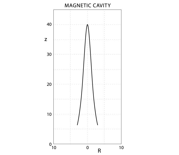
Figure 4.: The magnetic cavity occupied by the field becomes systematically taller with time but its lateral extent remains the same.

The stability of the towers is an interesting subject that cannot be treated here. However, some general guidance can be given. Long thin towers in compression are unstable to sideways buckling like an Euler strut. If by contrast they are in tension, they are stable to such buckling. However, even a liquid is stable under compression if it is surrounded by other liquid at the same pressure. Thus if we imagine a long thin tower of liquid it will only buckle if asked to support a pressure in excess of the ambient pressure of the surrounding liquid. From this example it is reasonable to expect our magnetic towers to buckle only if they experience a net compressive force greater than the ambient pressure. With $(\langle B^{2}_{\phi}\rangle-\langle B^{2}_{z}\rangle)/8\pi-p_{0}=0$ our towers are just stable by that criterion. However, we have neglected two other effects. Firstly, magnetic field is buoyant, so if $p_{0}$ decreases with height this should require a net tension from the magnetic stresses. Secondly, ram pressure at the head of any advancing jet will require some extra compression along the jet. As these two effects act in opposite directions we must leave the stability of the towers undecided. Finally, it is not clear that all real jets are stable to buckling; that of 3C273 appears bent on milliarcsecond scales.

4. Conclusions

In reality jets are dynamic whereas the towers we have calculated are static. In so far as the ram pressure and other inertial effects can be neglected, evolution through growing towers gives a realizable model. But such models which are very useful for guidance and understanding, should not be considered as giving the exact shapes to be expected from fully dynamic jets. However, they do supply an interesting and provocative answer to the question “Why are there jets at all?” Theories of jet models that fail to answer that question but assume an imposed flux of material from their base may be missing this point. Our picture also gives a good explanation of why jets advance at speeds directly related to the circular or escape velocity of the inner parts of the disks from which they emerge.

References

Aly, J. J. 1995, ApJ, 439, L63

Ambartsumian, V. A., & Shakbazian, R. K. 1958, Comm. Akad. Nunk. Armenin. SSR, 26, 277

Appl, S., & Camenzind, M. 1993, A&A, 270, 71

Bardeen, J. 1970, Nat, 226, 64

Beckwith, S. V. W., Sargent, A. L., Chin, R. S., & Gusten, R. 1990, AJ, 99, 924

Begelman, M. C., & Li, Z.-Y. 1994, ApJ, 426, 269

Bell, A. R., & Lucek, S. G. 1995, MNRAS, 277, 1327

Blandford, R. D., & Payne, D. G. 1982, MNRAS, 199, 883

Blandford, R. D., & Rees, M. J. 1974, MNRAS, 169, 395

Blandford, R. D., & Znajek, R. L. 1977, MNRAS, 179, 433

Bontemps, S., André, P., Terebey, S., & Cabrit, S. 1996, A&A, 311, 858

Bouvier, J. 1990, AJ, 99, 946

Burbidge, G. R. 1959, in IAU Symp. 9 & URSI Symp. 1, Paris Symposium on Radio Astronomy, ed. R. N. Bracewell (Stanford: Stanford University Press), p. 541

Burrows, C. J., et al. 1996, ApJ, 473, 437

Clarke, A. M. 1917–, in The Dictionary of National Biography, XIII, ed. L. Stephen & S. Lee (London: Oxford University Press), p. 333

Curtis, H. D. 1918, Publ. Lick Obs., 13, 31

Eddington, A. S. 1922, The Mathematical Theory of Relativity (Cambridge: Cambridge University Press), p. 162

Ekers, R. D., & Lynden-Bell, D. 1971, Astrophys. Letts., 9, 189

Gilham, S. 1981, MNRAS, 195, 753

Greenstein, J. L., & Schmidt, M. 1964, ApJ, 140, 796

Hargrave, P.J., & Ryle, M. 1974, MNRAS, 166, 305

Hazard, C., Mackay, M. B., & Shimmins, A. J. 1963, Nat, 197, 1037

Herschel, W. 1786, Phil. Trans., 76, 437

Heyvaerts, J., & Norman, C. A. 1989, ApJ, 347, 1055

Laplace, P. S. 1795, Système du Monde, Paris, p. 305

Laplace, P. S. 1809, System of the World, transl. J. Pond (London: Phillips)

Lery, T., Heyvaerts, J., Appl, S., & Norman, C. A. 1998, A&A, 337, 603

Li, H., Lovelace, R. V. E., Finn, J. H., & Colgate, S. A. 2001, preprint

Lovelace, R. V. E. 1976, Nat, 262, 649

Lucek, S. G., & Bell, A. R. 1996, MNRAS, 290, 327

Lynden-Bell, D. 1969, Nat, 223, 690

Lynden-Bell, D. 1971a, in Pontificiae Academiae Scientiarum Scripta Varia, Study Week on Nuclei of Galaxies, ed. D. J. K. O’Connell (New York: North-Holland Publishing)

Lynden-Bell, D. 1971b, MNRAS, 155, 95

Lynden-Bell, D. 1971c, MNRAS, 155, 119

Lynden-Bell, D. 1978, Phys. Scr., 17, 185

Lynden-Bell, D. 1986, in NATO Science Series B, vol. 186, Gravitation in Astrophysics, ed. B. Carter & J. B. Hartle (New York: Plenum), p.155

Lynden-Bell, D. 1996, MNRAS, 279, 389

Lynden-Bell, D., & Boily, C. 1994, MNRAS, 267, 146

Lynden-Bell, D., Priest, E. R., & Weiss, N. O. (eds.) 2000, Magnetic Activity in Stars, Disks & Quasars (Phil. Trans., 358, 635–867)

Lynden-Bell, D., & Rees, M. J. 1971, MNRAS, 152, 461

Margon, B. 1984, ARA&A, 22, 507

Mestel, L. 1968, MNRAS, 140, 177

Mestel, L. 1999, Stellar Magnetism (Oxford: Oxford University Press)

Mirabel, I. F., & Rodriguez, F. I. 1999, ARA&A, 37, 409

Michell, J. 1784, Phil. Trans., 74, 50

Miyoshi, M., Moran, J., Hernstein, J., Greenhill, I., Nakai, N., Diamond, P., & Inone, M. 1995, Nat, 373, 127

Narayan, R., & Yi, I. 1995, ApJ, 452, 710

Narayan, R., Barret, D., & McClintock, J. E. 1997, ApJ, 482, 448

Ne’eman, Y. 1965, ApJ, 141, 1303

Newton, I. 1704, Opticks (New York: Dover)

Novikov, I. D. 1964, A. Zh., 41, 1075

Okamoto, I. 1997, A&A, 326, 1277

Okamoto, I. 1999, MNRAS, 307, 253

Oke, J. B. 1963, Nat, 197, 1040

Ouyed, R., Pudritz, R. E., & Stone, J. E. 1997, Nat, 385, 409

Ouyed, R., & Pudritz, R. E. 1997, ApJ, 484, 794

Rees, M. J. 1971, Nat, 229, 312

Rosse, Earl of, 1850, Phil. Trans., 499

Ryle, M. 1968, Highlights of Astronomy, ed. L. Perek (Dordrecht: Reidel), p. 380

Sakurai, T. 1985, A&A, 152, 121

Sakurai, T. 1987, PASJ, 39, 821

Salpeter, E. E. 1964, ApJ, 140, 796

Sandage, A. R. 1965, ApJ, 141, 1586

Schmidt, M. 1963, Nat, 197, 1040

Schott, G. A. 1912, Electromagnetic Radiation and Reactions Arising from It, (Cambridge: Cambridge University Press)

Shakura, N. I., & Sunyaev, R. A. 1973, A&A, 24, 337

Shakura, N. I., & Sunyaev, R. A. 1976, MNRAS, 175, 613

Shibata, K., & Uchida, Y. 1985, PASJ, 37, 31

Shibata, K., & Uchida, Y. 1986, PASJ, 38, 631

Slipher, V. M. 1917, Lowell Obs. Bull., 3, 59

Tout, C. A., & Pringle, J. E. 1992, MNRAS, 259, 604

Vlahakis, N., & Tsinganos, K. 1998, MNRAS, 298, 777

Young, T. 1802, Phil. Trans., 92, 36