Time-resolved optical spectroscopy of the pulsating DA white dwarf HS 0507+0434B

We present a detailed analysis of time-resolved optical spectra of the ZZ Ceti white dwarf, HS 0507+0434B. Using the wavelength dependence of observed mode amplitudes, we deduce the spherical degree, $\ell$, of the modes, most of which have $\ell=1$. The presence of a large number of combination frequencies (linear sums or differences of the real modes) enabled us not only to test theoretical predictions but also to indirectly infer spherical and azimuthal degrees of real modes that had no observed splittings. In addition to the above, we measure line-of-sight velocities from our spectra. We find only marginal evidence for periodic modulation associated with the pulsation modes: at the frequency of the strongest mode in the lightcurve, we measure an amplitude of $2.6\pm 1.0$ kms^-1, which has a probability of 2% of being due to chance; for the other modes, we find lower values. Our velocity amplitudes and upper limits are smaller by a factor of two compared to the amplitudes found in ZZ Psc. We find that this is consistent with expectations based on the position of HS 0507+0434B in the instability strip. Combining all the available information from data such as ours is a first step towards constraining atmospheric properties in a convectionally unstable environment from an observational perspective.

1 Introduction

The apparent simplicity of white dwarfs belies more complex and ill-understood processes occurring in their interiors. Pulsations, however, offer the precious possibility of probing the interiors of these stars thereby yielding not only fundamental stellar parameters but also important clues of their prior history which can, in principle, be reconstructed from their present interior structure.

Along the white dwarf cooling track, there are three regions of instability: at $T_{\mathrm{eff}}\sim$ 110 kK, $T_{\mathrm{eff}}\sim$ 24 kK, and $T_{\mathrm{eff}}\sim$ 12 kK, populated by the GW Vir, V 777 Her (DBV), and ZZ Ceti (DAV) types, displaying strong lines in their optical spectra of He ii and C iv, He i, and H  respectively.

Given the relatively long pulsation periods of white dwarfs, the realisation that white dwarfs are non-radial gravity-mode pulsators (Chanmugam 1972; Warner & Robinson 1972) came soon after the discovery of the first variable white dwarf (Landolt 1968); that their photometric variations are primarily a manifestation of temperature perturbations rather than due to variations in geometry or surface gravity came only a decade later (Robinson et al. 1982).

In order to subject the ZZ Cetis to asteroseismological analysis and to provide constraints for pulsation models, it is crucial that the eigenmodes associated with the observed periodicities be identified. Observationally, this means determining the value of the spherical degree, $\ell$, and azimuthal order, $m$. A third quantity, not an observable, is the radial order $n$; it specifies the number of nodes in the radial direction and can only be inferred by detailed comparison of observed mode periods with those predicted by pulsation models.

Mode identification for the ZZ Cetis is fraught with difficulties. In part, the analysis has been hampered by an insufficient number of pulsation modes excited to observable levels and mode variability over several different time scales. For the vast majority of ZZ Cetis, results have remained somewhat ambiguous as the prerequisites for asteroseismological analysis were not met. Even the Whole Earth Telescope (WET) campaigns (Nather et al. 1990) on several objects (e.g. G 117-B15A, ZZ Psc, Kepler et al. 1995; Kleinman et al. 1998) were thwarted either by the small number of modes and lack of clear multiplet structure exhibited by these objects. Most efforts have focused on identifying similarities between the pulsational spectra of different stars to constrain the mode identification. This ultimately has a bearing not only on the determination of fundamental stellar properties but also on the mass of the superficial hydrogen layer (e.g. Bradley 1998). It is clear that there is an acute need for more direct and complementary methods of pinning down the identification of the eigenmodes.

To this end, Robinson et al. (1995) presented a method for inferring $\ell$ based on the the wavelength-dependence of limb darkening, due to which observed mode amplitudes vary with wavelength in a manner that depends on $\ell$, but not on any of the other properties of the pulsation mode, such as $m$ or amplitude. Thus, in a given star, modes having the same spherical degree will behave in the same manner. Robinson et al. (1995) acquired photometric data in the ultraviolet of the ZZ Ceti star G 117-B15A. Application of Bayes’ theorem and quantitative use of model wavelength-dependent pulsation amplitudes led them to infer that the largest amplitude mode of G 117-B15A had $\ell=1$.

More recently, van Kerkwijk et al. (2000) and Clemens et al. (2000) used a variant of the above method to identify the spherical degree of the pulsation modes observed in ZZ Psc (a.k.a. G 29-38) – a star that has been notoriously erratic in the pulsation modes that it excites. Their investigation, which was based on amplitude changes within the Balmer lines at visual wavelengths only, yielded empirical differences between the modes that were best interpreted as several $\ell=1$ modes and one $\ell=2$ mode; the presence of modes of differing $\ell$ obviated the need for quantitative model comparisons making their identification more secure than any previous attempt. A surprising by-product of their analysis was the detection of variations in the line-of-sight velocity associated with the pulsations. Given the instrumentation available at that time, these were thought to be too small to measure (Robinson et al. 1982).

The measurement of line-of-sight velocity variations associated with the pulsations can be used in two complementary ways: (i) they provide a means with which to verify and constrain the theories of mode driving and, (ii) under certain theoretical assumptions, velocity variations in conjunction with flux changes provide an important new tool with which to probe the outer layers of pulsating white dwarfs.

In this study, we will only attempt to interpret our observations within the context of theories of mode driving via convection (Brickhill 1983, 1991; Goldreich & Wu 1999a, b), as opposed to theories which purport mode driving by variants of the classical $\kappa$-mechanism (e.g. Dziembowski & Koester 1981; Dolez & Vauclair 1981; Winget et al. 1982). Unfortunately, as far as we are aware, testable predictions for these models are not, as yet, available.

Within the context of the “convective-driving” picture the convection zone responds to perturbations from the adiabatic interior on time scales very much shorter ($\sim\!1$ s) than the mode periods (hundreds of seconds). This allows the convection zone to absorb and release the flux perturbations cyclically, thus driving the pulsations. Combination frequencies (linear sums and differences of the real modes) arise naturally in the above picture and can, in principle, provide additional information. Furthermore, the relation between the flux and velocity variations allows one to estimate the total thermal capacity of the convection zone. Qualitative relations derived by Goldreich & Wu (1999a, b) show that these are also sensitive to $\ell$. We explore these issues in Sect. 7.

Based on the success of identifying the $\ell$ index of the modes of ZZ Psc using time-resolved spectroscopy, we present here, results from a similar analysis on HS 0507+0434B. Our primary aims are to attempt to determine the spherical degree ($\ell$) of the pulsations and to search for line-of-sight velocity variations associated with the pulsations. We also hope to constrain the properties of convection, a process which is poorly understood and therefore one of the main sources of uncertainty in the models.

We begin with a brief introduction to HS 0507+0434 in Sect. 2 followed by a description of the data in Sect. 3. In Sects. 4, 5, and 6, we attempt to extract the flux and velocity amplitudes and phases and the change in pulsation amplitudes with wavelength. From Sect. 7 onwards, we apply the constraints provided by all of the above to extricate quantities that allow us to both test and subsequently use the theory.

2 HS 0507+0434

HS 0507+0434, like many other white dwarfs, is the by-product of a survey for faint blue objects (the Hamburg Quasar Survey in this case). It comprises two DA white dwarfs in a common proper-motion pair which, as discussed by Jordan et al. (1998), is of particular interest for two reasons. First, the effective temperatures of 20 kK for HS 0507A and 11.7 kK for HS 0507B are such that the atmosphere of the former is completely radiative, while the latter has an outer convection zone. Thus, one can hope to use the parameters inferred from HS 0507A, which should be secure – since radiative atmospheres consisting of pure hydrogen are well understood – to calibrate models for HS 0507B, which have to rely on uncertain models for convection. Jordan et al. (1998) found that only with relatively inefficient versions of the Mixing Length Theory (MLT) were they able to find consistent solutions for both components in the system.

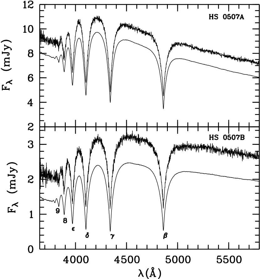
Figure 1: Sample and average spectra of HS 0507A and B in the 3650–5800 Å range with the Balmer lines indicated. The average spectra are offset from the sample spectra by 1 mJy and 0.65 mJy for the A and B components respectively.

The second reason that HS 0507+0434 is of interest is that the temperature of HS 0507B – as derived from its spectrum – placed it squarely within the ZZ Ceti instability strip; fast photometry on this object revealed it, as expected, to be variable (Jordan et al. 1998). A study of the temporal behaviour of HS 0507+0434B, based on photometric measurements collected over a total of seven consecutive nights, was recently carried out by Handler & Romero-Colmenero (2000). These authors were able to resolve a set of three equally spaced triplets. Under the assumption that the splitting was due to the effect of slow rotation on $\ell=1$ modes, the observed triplets yielded an estimate of the rotation rate ($\sim\!1.5\,$days) and the $m$ values of the multiplets. They also found that in all three triplets, the $m=0$ component was much weaker than the $m=-1$ and $m=+1$ components, which were of roughly similar strength. Assuming that the intrinsic amplitudes were the same for all $m$ components, they estimated the inclination of the rotation axis with respect to the line of sight to be $\sim\!79\degr$. The independent $\ell$ identifications afforded by clearly split multiplets are highly desirable as they can help to validate the identifications that rely on time-resolved spectroscopy only, given the differences between model spectra and observations.

As will become clear in the following sections, the advantage of having a flux and velocity reference in the same slit as the target greatly increases the accuracy of subsequent measurements by making it possible to not only divide out atmospheric fluctuations, but also to ensure that small random movements of the target in the slit are accounted for in the determination of the Doppler shifts of the Balmer-lines, thus making HS 0507+0434 an ideal system on which to test theoretical predictions.

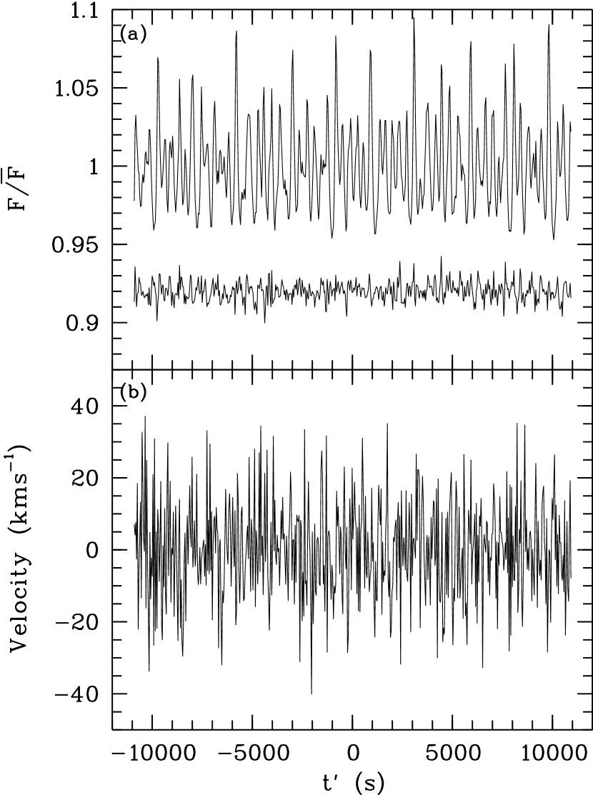
Figure 2: Light and velocity curves of HS 0507B, shown here for the first night only for the sake of clarity. t^′ = t$-$10:15:14 U.T. i.e. relative to the midpoint of the time series. (a) Fractional variations in the continuum region between $\sim$ 5300 – 5800 Å. The variations are with respect to the continuum of HS 0507A in the same wavelength region. Note that the maxima are stronger and sharper than the minima as is typical for ZZ Ceti type pulsators. The bottom curve shows the residuals (offset by $+$0.92) after fitting 26 sinusoids with amplitudes larger than 0.15% (see Table LABEL:hstab); (b) variations in the line-of-sight velocity also with respect to HS 0507A – as derived from fitting profiles to H$\beta$, H$\gamma$, and H$\delta$. No obvious variations are present and indeed we detect only marginal velocity variations associated with the pulsation modes (Sect. 5).

3 Observations and Data reduction

HS 0507+0434 was observed on the nights of $10^{\mathrm{th}}$ and $11^{\mathrm{th}}$ December 1997 using the Low Resolution Imaging Spectrometer (LRIS) on the Keck II telescope (Oke et al. 1995). An 8$\aas@@fstack{\prime\prime}$7-wide slit was used together with a 600 line mm^-1 grating covering the 3450-5960 Å range at 1.25 Å pixel^-1. On-chip binning by a factor of two was implemented in the spatial direction. The first night was photometric and the seeing of 1$\aas@@fstack{\prime\prime}$2 set the wavelength resolution to 7 Å. There were thin patches of cirrus on the second night; furthermore, there was a great deal of windshake, which resulted in a worse resolution (9 Å) although the situation improved towards the end of the run as the elevation decreased. A contiguous set of 560 24 s exposures were acquired from 7:13:35 to 13:17:17 U.T. on the first night and a further 280 exposures were obtained from 7:10:50 to 10:12:24 U.T. on the following night. For both nights, the series was preceded by exposures of the flux standard G 191-B2B (five and ten integrations of 4 s respectively), followed by HgKr arc spectra for wavelength calibration, and halogen flat-field frames. A total of 64 frames from the second night had to be discarded due to a malfunction of the guider, which resulted in the targets drifting off the slit. We decided to fix the slit at the position angle required to have both components of the system in the slit and deal with the effects of differential refraction during the reduction of the data. The decision to use a wide slit stemmed from the need to acquire ‘photometric’ measurements of HS 0507 A and B in addition to measurements of variations in the line-of-sight velocity (see Sect. 4).

The reduction of the data was carried out using MIDAS and using routines running in the MIDAS environment written specifically for the LRIS instrument and this data set. In detail, our reduction procedure entailed: (i) subtracting the CCD bias level of each amplifier separately using the overscan region; (ii) correcting for the (small) non-linearities that most CCDs are prone to, using linearity curves of the CCD derived from previous observations using the LRIS instrument; (iii) correcting for the gain difference between the 2 amplifiers as derived from halogen lamp frames; (iv) flat-fielding using an average of the halogen frames for the first night and an average of dome-flats for the second night (as these gave smoother results); (v) sky subtraction; (vi) correcting for the error introduced by dividing by a flat field taken through slightly non-parallel slits (described in more detail below); (vii) optimal extraction of the spectra using a method akin to that of Horne (1986); (viii) wavelength calibration using Hg/Kr frames (by tabulating wavelengths for each pixel rather than by rebinning the spectra), with an offset determined from star A, and including a correction for refraction (see below); and (ix) flux calibration with respect to the flux standard G 191-B2B, using the model fluxes of Bohlin et al. (1995) and using the extinction curve of Beland et al. (1988) to correct for small differences in airmass.

Among the usual preprocessing stages described above, two additional non-standard steps were required given our use of a wide slit, namely the need to correct for non-parallel slit-jaws and the need to account for the effects of random stellar wander in the slit due, for instance, to seeing-related changes, windshake, and tracking uncertainties.

Figure 3: (a) Fourier transform of the light curve (top) and residuals (bottom) offset by $-$0.2%. The maximum amplitude of peaks longward of 9000$\mu$Hz is $\sim$ 0.09%. (b) Fourier transform of the velocity curve. The frequencies inferred from the light curve are indicated. None of the frequencies present in the light curve have obviously significant associated velocity modulation. This is confirmed by our detailed analysis (Sect. 5), with the possible exception of F2, for which we find that associated signal has a probability of only 2% of being due to chance, constituting a marginal detection. (Note that without prior information from the light curve regarding which frequencies to expect, this peak would also be insignificant). Both (a) and (b) have been constructed using data from both nights.

The former correction is necessitated by the fact that while the flat-fields and sky background are influenced by the shape of the slit, the light from the targets is not, as no light falls outside the slit jaws. The sky background was determined by fitting first degree polynomials for each step along the dispersion direction excluding two regions of 26 and 30 binned pixels corresponding to HS 0507A and HS 0507B respectively, and multiplying the result by a function describing the shape of the slit. Finally, we divided the images by an average flat field frame that was normalised along the spatial direction in order to maintain the correct relative flux ratio between the two target objects.

A second non-standard correction is required to purge the data of any extraneous effect that introduces shifts in the positions of the Balmer lines, such as instrumental flexure, refraction, and wander. In principle, all these changes should affect HS 0507A and B in the same way, and one could simply measure wavelengths relative to HS 0507A only. However, we prefer the following methodology, as it not only permits us to assess the quality that one may expect in the absence of such a fortuitous local calibrator, but it also permits us to verify the stability of HS 0507A and provides insight into any systematic effects that may have crept into our analysis of other targets. We first correct the spectra of both stars for instrumental flexure and refraction and only then apply a correction for stellar wander, using the measured offsets of H$\gamma$ of HS 0507A as fiducial points. Having thus corrected each pixel in the spectrum for the effects of instrumental flexure, differential refraction, and random wander in the slit, we redid the wavelength and flux calibrations. Any remaining offsets of the Balmer lines from their respective laboratory wavelengths must now be due to intrinsic variations only.

An estimate of the remaining scatter due to wander in the derived velocities can be obtained from the shifts in the slit of the spatial profiles of both HS 0507A and HS 0507B and assuming that the scatter in these shifts is also representative of the scatter in the dispersion direction. Having fitted Gaussian functions to the spatial profiles, we take the standard deviation of the difference of the resulting centroid positions of HS 0507B with respect to those of HS 0507A as an indicator of the scatter and obtain a value of $\sim$2$\rm km\,s^{-1}$at H$\gamma$ as an average value for both nights. This is well below the measurement errors (see Sect. 5). Note that the root-mean-square scatter for ZZ Psc was 14 $\rm km\,s^{-1}$at H$\gamma$ (van Kerkwijk et al. 2000). The value of having a reference object in the slit thus cannot be overemphasized.

The final average spectra of HS 0507+0434 A and B, as well as sample individual spectra, are shown in Fig. 1.

Table 1: Pulsation frequencies and other derived quantities from the light and velocity curves of HS 0507B

	Mode	Period	Frequency	$\Phi_{L}$	$A_{L}$	$A_{V}$	$\Phi_{V}$	$R_{V}$	$\Delta\Phi_{V}$
		(s)	($\mu$Hz)	(°)	(%)	($\rm km\,s^{-1}$)	(°)	(Mm rad${}^{-1})$	$(\degr)$
Real Modes:
{	F1 ($f_{10}$) $m$ = $-$1	354.9 $\pm$ 0.03	2817.5 $\pm$ 0.3	0$-$27 $\pm$ 4	0.68 $\pm$ 0.11	2.0 $\pm$ 1.0	0$-$61 $\pm$ 29	17 $\pm$ 9	$-$088 $\pm$ 29
	F2 ($f_{8}$) 0$m=-1$	355.8 $\pm$ 0.02	2810.9 $\pm$ 0.2	0$-$57 $\pm$ 1	2.27 $\pm$ 0.06	2.6 $\pm$ 1.0	0$-$13 $\pm$ 23	06 $\pm$ 3	$-$044 $\pm$ 23
	F3 ($f_{2}$) 0$m=-1$	557.7 $\pm$ 0.03	1793.2 $\pm$ 0.1	00$-$6 $\pm$ 1	1.87 $\pm$ 0.04	0.8 $\pm$ 0.8	$-$$\cdots$	04 $\pm$ 4	$-$$\cdots$
	F4 ($f_{1}$)	743.0 $\pm$ 0.13	1346.1 $\pm$ 0.2	$-$153 $\pm$ 2	1.39 $\pm$ 0.04	0.3 $\pm$ 1.1	$-$$\cdots$	02 $\pm$ 9	$-$$\cdots$
{	F5 ($f_{5}$) 0$m=-1$	446.2 $\pm$ 0.05	2241.1 $\pm$ 0.2	0$-$0.2 $\pm$ 3	1.10 $\pm$ 0.09	1.6 $\pm$ 1.1	$-$$\cdots$	10 $\pm$ 7	$-$$\cdots$
	F6 ($f_{7}$) 0$m$ = $-$1	444.8 $\pm$ 0.06	2248.4 $\pm$ 0.3	0$-$74 $\pm$ 3	1.36 $\pm$ 0.07	2.3 $\pm$ 1.1	0$-$79 $\pm$ 26	12 $\pm$ 5	$-$004 $\pm$ 27
	F7	286.1 $\pm$ 0.04	3495.8 $\pm$ 0.5	$-$147 $\pm$ 6	0.36 $\pm$ 0.04	0.8 $\pm$ 0.8	$-$$\cdots$	09 $\pm$ 9	$-$$\cdots$
Combination Modes:
	Mode	Period	Frequency	$\Phi_{L}$	$A_{L}$	$A_{V}$	$\Phi_{V}$	$R_{C}$	$\Delta\Phi_{C}$
		(s)	($\mu$Hz)	(°)	(%)	($\rm km\,s^{-1}$)	(°)		(°)
	F4+F6	0278.2	3594.4	$-131\pm\phantom{0}4$	0.80 $\pm$ 0.05	0.9 $\pm$ 1.1	$-$$\cdots$	20.7 $\pm$ 1.8	0$-53\pm\phantom{0}5$
	F1+F3	0216.9	4610.7	0$-$32 $\pm$ 07	0.38 $\pm$ 0.04	0.2 $\pm$ 1.0	$-$$\cdots$	15.0 $\pm$ 3.0	00$-$1 $\pm$ 08
	F2+F3	0217.2	4604.2	0$-$73 $\pm$ 08	0.30 $\pm$ 0.05	1.1 $\pm$ 1.0	$-$$\cdots$	03.5 $\pm$ 0.6	0$-$10 $\pm$ 08
	F2+F4	0240.6	4156.8	$-$129 $\pm$ 11	0.20 $\pm$ 0.04	0.4 $\pm$ 0.8	$-$$\cdots$	03.0 $\pm$ 0.6	0$-$21 $\pm$ 12
	F3+F6	0247.4	4041.7	0$-$71 $\pm$ 08	0.33 $\pm$ 0.04	1.0 $\pm$ 1.0	$-$$\cdots$	06.4 $\pm$ 0.9	00$-$2 $\pm$ 08
	F3+F5	0247.9	4034.4	0$-$57 $\pm$ 17	0.16 $\pm$ 0.04	0.4 $\pm$ 1.1	$-$$\cdots$	03.9 $\pm$ 1.1	0$-$51 $\pm$ 17
	F1+F5 [F2+F6]	0197.7	5058.6	0$-$12 $\pm$ 04	0.50 $\pm$ 0.04	1.4 $\pm$ 0.8	$-$$\cdots$	32.8 $\pm$ 6.2	0$-$15 $\pm$ 07
	F2$-$F4	0682.6	1464.9	0$-$41 $\pm$ 06	0.37 $\pm$ 0.04	1.3 $\pm$ 0.8	$-$$\cdots$	05.9 $\pm$ 0.6	0$-$55 $\pm$ 06
	F5+F6	0222.7	4489.6	0$-$80 $\pm$ 08	0.27 $\pm$ 0.04	0.8 $\pm$ 0.8	$-$$\cdots$	09.0 $\pm$ 1.5	00$-$5 $\pm$ 09
	F1+F2	0177.7	5628.4	$-$140 $\pm$ 10	0.21 $\pm$ 0.04	0.5 $\pm$ 0.8	$-$$\cdots$	06.7 $\pm$ 1.6	0$-$57 $\pm$ 11
	F3$-$F4 [F5$-$F3]	2236.5	0447.3	$-$102 $\pm$ 09	0.23 $\pm$ 0.04	0.3 $\pm$ 0.8	$-$$\cdots$	04.3 $\pm$ 0.7	$-$111 $\pm$ 10
	F1$-$F5	1735.0	0576.4	$-$144 $\pm$ 10	0.22 $\pm$ 0.04	0.9 $\pm$ 0.8	$-$$\cdots$	14.4 $\pm$ 3.5	$-$170 $\pm$ 11
	F3+F4	0318.6	3139.2	$-$160 $\pm$ 11	0.19 $\pm$ 0.04	1.0 $\pm$ 0.8	$-$$\cdots$	03.6 $\pm$ 0.7	0$-$41 $\pm$ 11
	2F3 [F4+F5]	0278.8	3586.5	$-$128 $\pm$ 17	0.19 $\pm$ 0.05	1.4 $\pm$ 1.0	$-$$\cdots$	05.4 $\pm$ 1.5	$-$116 $\pm$ 17
	F1+F2+F3	0134.7	7421.6	$-$128 $\pm$ 14	0.16 $\pm$ 0.04	0.3 $\pm$ 0.8	$-$$\cdots$	090 $\pm$ 30	0$-$38 $\pm$ 14
	F2+F4+F6 [2F3+F1]	0156.1	6405.2	$-$151 $\pm$ 07	0.28 $\pm$ 0.04	0.7 $\pm$ 0.8	$-$$\cdots$	108 $\pm$ 16	0$-$74 $\pm$ 08
	F3+F4+F6	0185.6	5387.6	$-$152 $\pm$ 08	0.25 $\pm$ 0.04	0.7 $\pm$ 0.8	$-$$\cdots$	117 $\pm$ 19	$-$124 $\pm$ 09
	2F4+F6	0202.4	4940.3	0$-$14 $\pm$ 13	0.17 $\pm$ 0.04	1.8 $\pm$ 0.8	$-$$\cdots$	208 $\pm$ 50	$-$143 $\pm$ 14
	F4+F6$-$F5 [$m$=1, F4]	0739.0	1353.3	00$-$1 $\pm$ 18	0.24 $\pm$ 0.05	1.3 $\pm$ 1.0	$-$$\cdots$	190 $\pm$ 43	$-$079 $\pm$ 18

Notes. The frequencies listed in brackets next to the real modes refer to the nomenclature preferred by Handler & Romero-Colmenero (2000). The curly brackets next to two pairs of real modes indicate that these are multiplets sharing the same $\ell$ but differing $m$ values (see also Sect. 7.2). We have followed the convention that positive values of $m$ correspond to prograde modes. $R_{V}=A_{V}/(2\pi fA_{L})$, in units of Mm rad^-1, has the physically intuitive meaning of being the typical distance a fluid element travels on the surface for a pulsation with a fractional amplitude of unity. $\Phi_{L}$ and $\Phi_{V}$ are the phases of the sinusoids fit to the light and velocity curves respectively with $\Delta\Phi_{V}=\Phi_{V}-\Phi_{L}.$ For the combination frequencies, $R_{C}=A_{L}^{i\pm j}/(n_{ij}A_{L}^{i}A_{L}^{j})$ where $n_{ij}$ is unity for $i=j$, 2 for 2-mode combinations etc. and 3 for 3-mode combinations involving the first harmonic, e.g. 2F4+F6. $\Delta\Phi_{C}=\Phi_{L}^{i\pm j}-(\Phi_{L}^{i}\pm\Phi_{L}^{j}$). Potentially misidentified modes are listed in square brackets next to the combination modes. Note that this list is not an exhaustive one. The frequency of the combination F4+F6$-$F5 is at the location of the $m=1$ multiplet c.f. F4 (we infer in Sect. 6 that F4 has $\ell=1$ and in Sect. 7.2 that it probably has $m=-1$).

4 Periodicities in the Light Curve

Continuum light curves for each night were constructed by dividing the average flux in the 5300–5800 Å region of HS 0507B by that of HS 0507A (see Figs. 1, 2a). Note that the time axis has been computed relative to the middle of the time series in order to minimize any covariance between the frequencies and phases of the sinusoids we subsequently use to fit the light curve ($t^{\prime}=t-16:33:20$ U.T.). The Fourier transform of the light curve obtained by merging the data from both nights is shown in Fig. 3a and is typical of that of the ZZ Cetis.

We determined the periodicities consecutively in terms of decreasing amplitude by means of an iterative process: using an approximate value for the frequency of the highest peak, we fitted a function of the form $A\cos(2\pi ft^{\prime}-\phi)+C$ where $A$ is the amplitude, $f$ the frequency, $\phi$ the phase and $C$, a constant offset. The fit yielded $A$, $f$ and $\phi$. The process was repeated, adding a new sinusoid each time, and fitting for all parameters simultaneously until no peaks with amplitudes $\ga 0.15\%$ could be identified in the Fourier transform of the residuals.

Combination frequencies were identified by searching for linear combinations of the real modes and these were fitted by fixing the frequencies to those of the corresponding combination of the real mode frequencies. We imposed the requirement that the combination frequency in question have the smallest amplitude of the frequencies involved. Identification of combination frequencies was not always easy due to degenerate combinations (e.g. F3$-$F4 $\simeq$ F5$-$F3 given our resolution). In such cases, we opted for the largest amplitude of the combination frequency and the lowest possible error yielded by the fit. The light curve is not free of periodicities after having subtracted the frequencies listed in Table LABEL:hstab; although we continued to fit further combination modes, we found that the choice of combinations became rather arbitrary and hence we do not report these here.

Two statements can already be made on the basis of Table LABEL:hstab. First, as F1 and F2 have the same splitting as the F5 and F6 multiplet components, they therefore very probably also share the same $\ell$ value. From the analysis of Handler & Romero-Colmenero (2000), who detect triplets in each of these groups, they are likely to have $\ell=1$ and $m=\pm 1$. Second, the periods of the real modes are very similar to those observed by Kleinman et al. (1998) in a time series spanning 10 years for ZZ Psc, a similar, but slightly cooler white dwarf. In that star, these authors find real modes at periods ranging from 110 - 915 s. For $\ell=1$, these correspond to successive radial orders ($n$) from 1 to 18. The modes in common with HS 0507B are at 284, 355, and 730 s, which they identify as having radial orders of 4, 5, and 13 respectively. The $n$ = 7 mode in their model is the only mode (from $n$ = 1 - 18) not detected in the ZZ Psc data. Interestingly, a mode at the expected frequency is present in HS 0507B as the F5,F6 multiplet pair (445 s) at the expected separation for $\ell=1$ modes. It is tempting to conclude that, as for the hot ZZ Cetis (Clemens 1993), the cool ZZ Cetis have remarkably similar structure. One should bear in mind, however, that similar period structures may well be produced for a number of different combinations of mass and hydrogen-layer thickness (e.g. Bradley 1998).

We refrain from a detailed comparison with the study of Handler & Romero-Colmenero (2000) given our lower frequency resolution, but a few points are noteworthy. While the frequencies of the modes detected in our data are entirely consistent with those found by Handler & Romero-Colmenero (2000), our lower resolution does not permit us to confirm the presence of the $m=0$ multiplet components independently (see Fig. 4a); these were also the weakest modes in all triplets and thus should not greatly influence the amplitudes of the $m=\pm 1$ components. As a check, we attempted to recover the real modes identified by Handler & Romero-Colmenero (2000) that were not detected by us, by first imposing the amplitudes and frequencies listed by Handler & Romero-Colmenero (2000) and subsequently leaving the amplitudes free to vary. The residuals are shown in Fig. 4b. We find that our data are consistent with all but one of the components and have amplitudes consistent with those derived by Handler & Romero-Colmenero (2000). The only exception is the $m=1$ mode at 1800.7 $\mu$Hz (in the same multiplet as our F3), for which Handler & Romero-Colmenero (2000) found an amplitude of 1.7%, while it has an amplitude of only $\la\!0.5\%$ in our data and is not even required in the fit. For completeness, we note that the amplitudes and phases we derive using the frequencies of Handler & Romero-Colmenero (2000) are entirely consistent with those listed in Table LABEL:hstab.

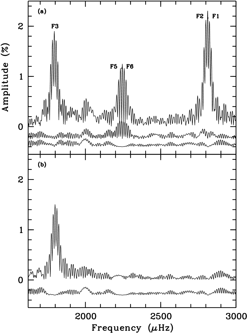
Figure 4: (a) The top curve shows the FT of the light curve in the $1600-3000\,\mu$Hz range. The middle curve shows the FT of the residuals after subtracting sinusoids with frequencies corresponding to all real modes except F1 and F6, which are multiplets in the same period group as F2 and F5 respectively, while the bottom curve shows the effect of including F1 and F6 in the fit. These two lower curves have been offset by $-$0.25% and $-$0.40% respectively. While there are some feeble signs of residual modulation around F1 and F2, this is clearly not the case for F5 and F6. Fitting an additional sinusoid near the F1,F2 pair in the hope of recovering the missing component is of no avail. (b) Top curve: residuals in the FT after subtracting three sets of triplets with frequencies and amplitudes fixed to those listed in Handler & Romero-Colmenero (2000). The large residual corresponds to the $m=1$ mode at 1800.7$\mu$Hz showing that the amplitude of this mode has changed considerably since our observations, from 1.7 to $\lesssim 0.5$%. The bottom curve (offset by $-$0.3%) shows the effect of leaving the amplitudes free to vary while leaving the frequencies fixed.

5 Periodicities in the line-of-sight velocities

Variations in the equivalent widths and profiles of the Balmer lines reflect temperature and line-of-sight velocity variations. The details of the complex interactions between flux and velocity that result in the observed spectral line are not well-understood, but are likely to be separable to first order.

In order to search for line-of-sight velocity variations, we determined Doppler shifts for the Balmer lines by fitting a combination of a Gaussian and a Lorentzian profile which provided a good fit to the lines; the continuum was approximated by a line. We chose the wavelength intervals 4660$-$5088 Å, 4214$-$4514 Å, and 4028$-$4192 Å for H$\beta$, H$\gamma$, and H$\delta$ respectively to carry out the fits and insisted that the central wavelengths of the Gaussian and Lorentzian functions be the same. We repeated the above process for H$\gamma$ only, fitting the logarithm of the flux instead as a check of our (additive) fitting method. The velocities thus derived were nearly identical with those obtained by fitting the flux only. Possible systematic effects arising from different methods of deriving these velocities are discussed in detail in van Kerkwijk et al. (2000). The resulting velocity curve is shown in Fig. 2b, while the associated Fourier transform is shown in Fig. 3b. The typical uncertainty in a single measurement for HS 0507B is 14 $\rm km\,s^{-1}$, much larger than those due to differential wander between HS 0507A and B which was estimated to be $\la$ 2 $\rm km\,s^{-1}$(Sect. 3).

Simple checks confirm that the errors in the measurement of the line-centroids of each of the three Balmer lines are uncorrelated. For instance, the standard deviation of the average velocity as computed from an average of all three lines decreases by a factor $(\sigma_{\beta}+\sigma_{\gamma}+\sigma_{\delta})^{\frac{1}{2}}$/3 compared to that associated with a single line, as would be expected if the errors were mutually independent (here, $\sigma_{\beta,\gamma,\delta}$ are the respective standard deviations in the velocities as derived from H$\beta$, H$\gamma$, and H$\delta$). The velocity differences between the lines also offer an independent estimate of the measurement uncertainty; e.g. one expects the ratio $(v_{\beta}-v_{\gamma})/(\sigma_{\beta}^{2}+\sigma_{\gamma}^{2})^{\frac{1}{2}}$ to have a mean of zero and a standard deviation of unity if the errors associated with each line are uncorrelated. Our values of the standard deviation of the above ratio for the two nights are 1.2 and 1.3, i.e., roughly consistent with unity. We deem our error estimates to be credible.

The Fourier Transform of the velocity curve (Fig. 3b) is striking in that it shows no strong peak at any frequency, not even at the frequencies corresponding to the dominant variation in the light curve. We will explore the possible cause of this result in later sections. We can, nevertheless, place interesting upper limits on the velocity to flux ratio of each observed mode. The motivation for doing so is that the velocity to flux ratios ($R_{V}$) have, to date, only been determined for one star (van Kerkwijk et al. 2000); yet, these are essential for comparison with theoretical predictions. While the noise level prevents the velocity curve from being used in the absence of external information, the light curve provides just such external, independent, information as to the periodicities we expect to find in the velocity curve. We can exploit this additional information by imposing the frequencies we find in the light curve on the velocity curve and measuring the velocity amplitudes at these pre-specified frequencies. We can subsequently ask if a velocity peak at a known frequency is signficant. We detail this procedure below.

As just described, we looked for modulations in the velocity curve by fitting the velocity curve with sinusoids, the frequencies of which were fixed at those obtained from the light curve. As with the light curve, the calibration relative to HS 0507A removed all slow variations and only a constant offset was additionally included in the fit. The resulting velocity amplitudes and phases are listed in Table LABEL:hstab. We find marginally significant velocity variations at F1, F2, and F6. If these are real, it is surprising that we do not find significant velocity variations at F3 and F4, in spite of these modes having stronger flux modulations than F1 and F6. For F4, this is due in part to the proximity of the combination mode F4+F6$-$F5. Excluding all combination modes from the fit (theoretically, these are not expected to have associated velocity variations) results in an increase of the velocity amplitude of F4 to 0.8 $\rm km\,s^{-1}$ ($R_{V}=7\pm 7$) while the amplitudes for the other real modes change by less than 0.2 $\rm km\,s^{-1}$.

We carried out Monte Carlo simulations in order to ascertain the likelihood that the peaks as large as those we detected might occur simply by chance. Our simulations were conducted thus: we randomly distributed the velocities with respect to the times and then fit these velocity curves in exactly the same way as the observations i.e., by fixing the frequency of the sinusoids to those derived from fits to the light curve as described above. This procedure was repeated 1000 times and the number of peaks with amplitudes larger than those measured at the frequencies corresponding to the real modes were counted. The results corroborated our error estimates: the modulation at F2 was most significant, having a probability of only 2% of being a random occurrence, while the modulations at F1 and F6 had probabilities of 9% and 4% respectively of being chance occurrences. In what follows, we treat these measurements as upper limits.

In summary, we find that at the frequency of F2, the mode with the largest photometric amplitude, there is evidence for an associated velocity signal with an amplitude of $2.6\pm 1.0{\rm\,km\,s^{-1}}$, which our Monte-Carlo simulation suggests has a probability of only 2% of being due to chance. If taken at face value, we have thus detected velocity variations in a second ZZ Ceti type pulsator. A more conservative conclusion is that the upper limit to the velocity variations is $3{\rm\,km\,s^{-1}}$ (at 99% confidence). Before addressing what one can infer from the (limits to) the amplitudes, we first present a discussion of the chromatic amplitudes, from which we attempt to infer the spherical degree of the real modes.

6 Chromatic Amplitudes

Figure 5: Chromatic amplitudes for the 7 real modes and 2 of the stronger combination modes. The period is indicated next to the name. From photometry, we know that F1 and F2 are modes having the same $\ell$ but different $m$ values; likewise for F5 and F6. Note the shape and curvature of the continuum between the line-cores. The chromatic amplitudes confirm that at least the stronger modes share the same $\ell$ value (see also Fig. 7).

As was noted by Robinson et al. (1995), the wavelength dependence of the fractional pulsational amplitude, $\Delta\,F_{\lambda}/F_{\lambda}$, can potentially provide a clean measurement of the spherical degree ($\ell$) of the modes as it is not only independent of the inclination and $m$ (and therefore also to unresolved modes having the same $\ell$ but different $m$, but is also insensitive to the details of flux calibration.

We have computed these fractional pulsation amplitudes at each wavelength (hence the name, ‘chromatic amplitudes’) by fitting the real and combination modes listed in Table LABEL:hstab in each 3 Å bin, where the choice of bin size reflects a compromise between adequate signal to noise and resolution. The frequencies of the modes were fixed at the values shown in Table LABEL:hstab while the amplitudes of the modes were left free to vary. At first, we also left the phases free, but found that these did not show any significant signal. Since Clemens et al. (2000) found from their high signal-to-noise ratio data that the phases show very little variation, we decided to determine the amplitudes with the phases fixed to the values listed in Table LABEL:hstab. The resulting chromatic amplitudes are shown in Fig. 5 (allowing the phases to vary produces a very similar figure).

Clemens et al. (2000) were able to see a clear contrast between the chromatic amplitudes for their $\ell=1$ modes and that for the one $\ell=2$ mode present in their data for ZZ Psc. We see no such clear contrasts for HS 0507B (Fig. 5). Mostly, this simply reflects the fact that HS 0507B is about 8 times fainter, and that our signal-to-noise ratios are correspondingly lower. In Fig. 6, we compare the observed chromatic amplitudes for the strongest modes in HS 0507B (F2) and ZZ Psc (F1, $\ell=1$). We overlay model chromatic amplitudes for comparison. These were computed using model atmospheres (kindly provided by D. Koester; earlier versions described in Finley et al. 1997). The similarity of the displayed chromatic amplitude of HS 0507B and ZZ Psc and the dissimilarity of either to the models is striking. Pending improvements to the models, we must invent other methods to distinguish between $\ell=1$ and $\ell=2$ modes.

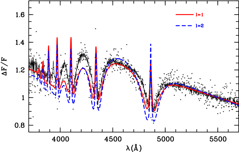
Figure 6: Comparison between observed and model chromatic amplitudes for the strongest mode of HS 0507B (F2, dots) and that of ZZ Psc (F1, full line) shown over a 2000 Å range only for clarity. F1 of ZZ Psc was identified as having $\ell=1$ by Clemens et al. (2000). The model chromatic amplitudes overlaid on the data are for T${}_{\rm{eff}}=12000$ kK, $\log g=8$ and ML2/$\alpha=0.6$. All amplitudes have been normalised such that they equal 1 at 5500 Å. The data for ZZ Psc are from Clemens et al. (2000).

A careful inspection of Fig. 5 reveals that F2, F3, F4, and F6 look qualitatively similar to each other while the continuum shape and curvature – especially between H$\beta$ and H$\gamma$ – are somewhat different for F7. Although the continuum between the line cores is not smooth for the weaker multiplets, the general shape of the line cores is not unlike that of the stronger modes. We focus upon these differences – the same ones found for ZZ Psc – in order to glean any clues on the spherical degree of the pulsation modes.

For ZZ Psc, two distinguishing features of the $\ell=1$ modes compared to the one $\ell=2$ mode were that the latter had a larger curvature in the continuum regions between the line cores and that the overall slope was steeper. In the hope of separating out modes having different $\ell$ values, we attempt to measure these two quantities by fitting a 2^nd-order polynomial between the lines cores as differences in these regions are readily apparent. We use ZZ Psc as a test case as at least one $\ell=2$ mode was identified by simple inspection.

In order to minimize the effect of local amplitude variations on the curvature and to minimize the covariance between the various parameters, we fit $y=y_{0}+y_{1}z+y_{2}z^{2}$, where $y=\ln a$ is the (natural) logarithm of the amplitude $a$ and $z=\ln\lambda-\langle\ln\lambda\rangle$, with $\langle\ln\lambda\rangle$ the average of $\ln\lambda$ in the wavelength region of interest. Here, we only show the results for the region between H$\beta$ and H$\gamma$ (4370–4820 Å). We also define $y_{0m}=(y_{0}-\langle\ln a\rangle_{5500})/(\langle\ln\lambda\rangle-\ln 5500)$. In this scheme, $y_{0m}$ can be seen to be a measure of the slope of the entire spectrum, while $y_{1}$ measures the local slope. Plotting $y_{2}$ against $y_{0m}$ should group together the modes that have similar shapes and curvatures.

Indeed Fig. 7 shows that F4 from the Clemens et al. (2000) data set clearly stands out from the cluster of $\ell=1$ modes. The situation is somewhat less clear-cut for HS 0507B: while F2, F3, F4, and F5 are consistent with each other and with F1 and F2 of ZZ Psc, the position of F6 is puzzling, although its value of $y_{0m}$ is consistent with that of the other strong modes. This, together with the general appearance of the chromatic amplitudes implies that F2, F3, F4, and F5 have $\ell=1$ and as F1 and F6 are members of known $\ell=1$ multiplets, they too must have $\ell=1$, even though this is not obvious from their respective locations in Fig. 7. The difference in appearance of F7 mentioned above is borne out by the measured slope and curvature. Given its low amplitude, we cannot unfortunately rule out the contribution of random noise. We note with interest that Handler (private communication) finds a peak of $\sim\,0.19$% at 3489.09 $\mu$Hz i.e. at approximately the same splitting as that observed for the 355 s and 445 s multiplets suggesting that F7 may be part of an $\ell=1$ triplet.

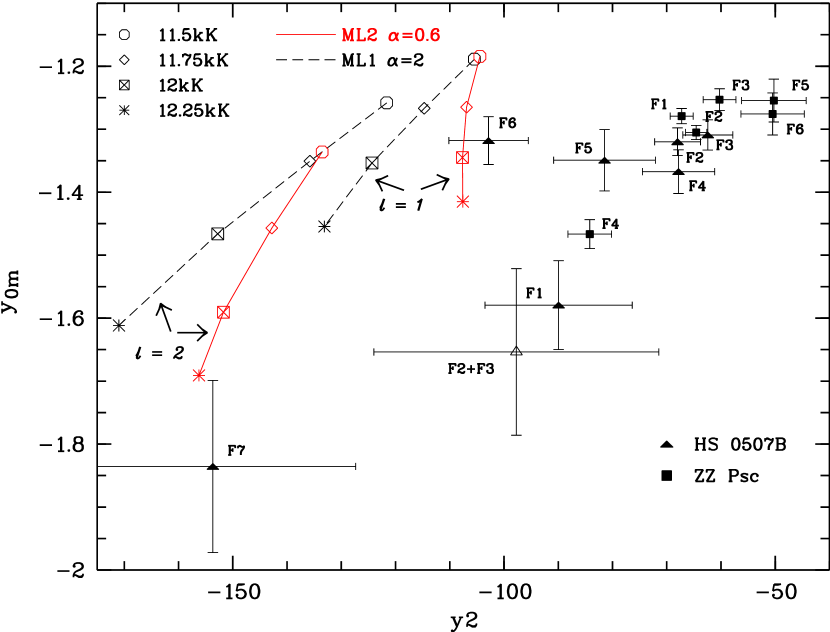
Figure 7: Measures of the observed (HS 0507, ZZ Psc) and model curvatures in the chromatic amplitudes between H$\beta$ and H$\gamma$. Energy transport by convection is comparable in the ML1/$\alpha$=2 and ML2/$\alpha$=0.6 versions. The model amplitudes were convolved with a Gaussian having a FWHM of 4.6 Å to match the seeing profile and extended over the 8$\aas@@fstack{\prime\prime}$7 slit.

We can check the reliability of the above method by repeating the procedure for those combination modes for which the $\ell$ character of the combination is known. The spherical harmonic character of combination modes can be deduced from selection rules whenever the $\ell$ and $m$ values of the constituent real modes is known. Thus for combinations involving two $m=1$ or $m=-1$ modes (for $\ell=1$), the resulting wavelength-dependent pulsation amplitude should have a surface distribution described by a $Y_{2}^{\pm 2}$ component and its position in Fig. 7 should coincide with F4 of ZZ Psc (which has $\ell=2$). Unfortunately, we do not have any independent knowledge of $m$ for any of the modes in ZZ Psc and cannot use its combination modes to verify the locations of the real modes in Fig. 7. Of our combination modes, F2+F3 is the largest amplitude one that satisfies the above $m$-requirement. Its location in Fig. 7 is roughly consistent with it having an $\ell=2$ component, although the uncertainties are too large for the measurement to be significant. In general, our conclusion from the above exercise is that although one obtains quantitative measures for the differences between modes having differing $\ell$ indices, it merely serves to corroborate the conclusions arrived at by visual inspection of the chromatic amplitudes.

As an aside, we note that using all the real modes listed in Table A1 in van Kerkwijk et al. (2000) results in one other mode, F8 ($920\pm 3$ s), being almost coincident with the position of the $\ell=2$ mode (F4, 776 s) in Fig. 7, while FA (500 s) is consistent with the position of F4 within the errors. Taken at face value, this implies that the 920 s mode also has $\ell=2$. Kleinman et al. (1998) assumed $\ell=1$ for their 918 s mode so it would be interesting to check the validity of this assumption by assigning a value of $\ell=2$ to this mode in the pulsation models and attempting to quantify the resulting changes, if any, to the derived properties of ZZ Psc. Given the relatively low amplitude of F8 (0.47%), other independent constraints would, of course, be desirable.

We repeated the above procedure on the model chromatic amplitudes for a range of temperatures and a number of different sets of mixing-length parameters. We show two examples in Fig. 7 one for ML2/$\alpha=0.6$, which was found to yield the best description of the average optical-to-ultraviolet spectra (Bergeron et al. 1995) and one for ML1/$\alpha=2.0$, which lies in the parameter space of models with which the observed magnitude difference between HS 0507A and B was best reproduced (Jordan et al. 1998); see Jordan et al. (1998) for a description of the terminology. We find that all models, like the two shown, have systematically higher curvature than the observations. Thus, we extend to all models the conclusion of Clemens et al. (2000) that while the salient features of the chromatic amplitudes are reproduced by the models, the details leave much to be desired. It may well be that better agreement will only be reached once a better description of convection becomes available.

7 Comparison with Pulsation Theory

In this section, we attempt to place our observations within a theoretical framework by comparing various quantities derived from our observations to those derived from theoretical considerations by Wu & Goldreich (1999), Goldreich & Wu (1999a), and Wu (2001). Our primary aim in this section is to check whether theoretical expectations are borne out by the observations for both real and combination modes. Our secondary aim is to use our observations to perform consistency checks on some of the theoretical parameters used in the above studies. Specifically, these parameters are the thermal time constant of the convection zone ($\tau_{c_{0}}$), and the parameter ($|2\beta+\gamma|$) that depends on the depth of the convection zone. We additionally check whether the inclination angle derived by Handler & Romero-Colmenero (2000) is consistent with our data. Before proceeding, we stress that any comparison with the theory is rendered difficult by a number of factors, in particular, by unresolved multiplets and by the presence of real and combination modes of low amplitude.

7.1 Real Modes

Following van Kerkwijk et al. (2000), we measure the relative flux and velocity amplitudes and phases of the real modes with $R_{V}=A_{V}/(2\pi fA_{L})$ and $\Delta\Phi_{V}=\Phi_{V}-\Phi_{L}$, respectively. In Table LABEL:hstab, we list the values of $R_{V}$ for all real modes. Here, one should bear in mind that the detection of even the strongest mode is only marginal. For the weaker modes, the $R_{V}$ values represent upper limits.

As a ZZ Ceti type white dwarf cools, the depth of the convection zone increases and longer period modes are excited. However, the flux perturbations are also more effectively attenuated so the emergent flux variations at the photosphere for a mode of fixed internal pulsation amplitude are reduced. Now turbulent viscosity in the convection zone ensures negligible vertical velocity gradients, making the horizontal velocities effectively independent of depth within the convection zone (Brickhill 1990; Goldreich & Wu 1999b). Thus at a fixed frequency, $R_{V}$ should be smaller in white dwarfs with thinner convection zones, i.e. the hotter pulsators. Similarly, for different modes within the same object, the flux attenuation increases with increasing mode frequency, while velocity variations pass undiminished through the convection zone. Thus $R_{V}$ is expected to increase with increasing mode frequency. $\Delta\Phi_{V}$ is expected to be equal to 90$\degr$ for the adiabatic case (flux leads maximum positive velocity by $\pi/2$) and to tend towards 0$\degr$ with increasing frequency, as the flux variations are increasingly delayed.

In Fig. 8, we show the observed values of $R_{V}$ and $\Delta\Phi_{V}$ for both HS 0507B and ZZ Psc. The observations are broadly consistent with expectations, in that the average values of $R_{V}$ are reasonable, and values of $\Delta\Phi_{V}$ are between 0 and 90$\degr$. We find no clear evidence, however, for the expected trends with frequency as the uncertainties are too large.

The longest period observed mode can be used to deduce a rough lower limit to the value of $\tau_{c_{0}}$, the thermal time constant of the convection zone, as the overstability criterion $\omega\tau_{c_{0}}\ga 1$ must be satisfied for driving to exceed damping (Goldreich & Wu 1999a). Using F4 from Table LABEL:hstab yields a value for $\tau_{c_{0}}$ of $\ga$118 s.

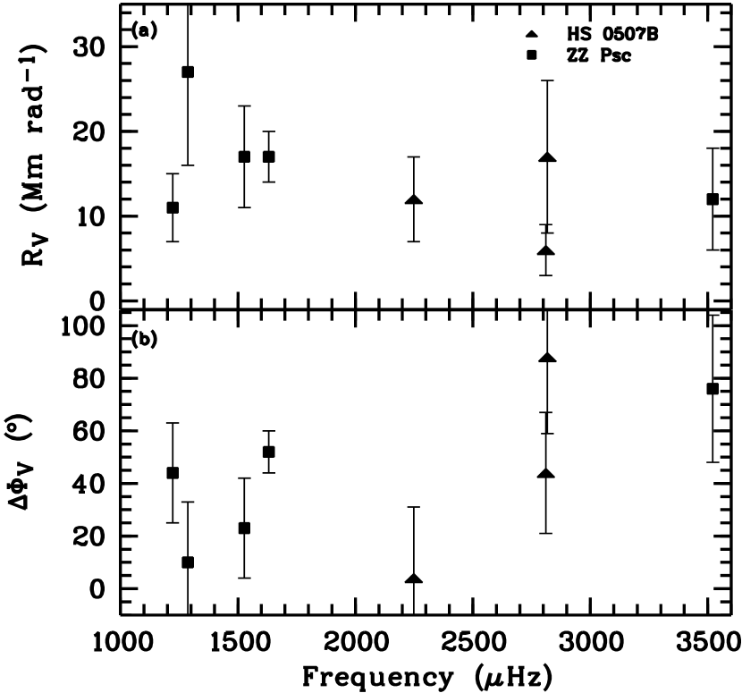
Figure 8: The relative velocity to flux amplitudes (a) and phases (b) for HS 0507B and ZZ Psc. The values for ZZ Psc are taken from Table 1 in van Kerkwijk et al. (2000).

7.2 Combination Frequencies

In models, the sharp maxima and shallower minima that typify the light curve are the result of the variation in the depth of the convection zone in response to the perturbations; this variation distorts the flux variation and gives rise to linear combinations of frequencies when transformed into frequency space (Brickhill 1992; Wu 2001). Thus, combination modes are not expected to have associated physical motion.

The relative photometric amplitudes and phases of the combination modes with respect to their constituent real modes can be expressed as $R_{C}=A_{L}^{i\pm j}/(n_{ij}A_{L}^{i}A_{L}^{j})$ where $n_{ij}$ is the factorial of the number of different modes in the combination for 2-mode combinations and $\Delta\Phi_{C}=\Phi_{L}^{i\pm j}-(\Phi_{L}^{i}\pm\Phi_{L}^{j}$) respectively. Relations linking theoretical quantities to observed ones are provided by Eq. (15) and (20) in Wu (2001). We quote these here for convenience:

$$\Delta\Phi_{C}=\tan^{-1}\left({1\over{(\omega_{i}\pm\omega_{j})\tau_{c_{0}}}}\right)$$ (1)

$$R_{C}={{|2\beta+\gamma|(\omega_{i}\pm\omega_{j})\tau_{c_{0}}}\over{4\alpha_{V}\sqrt{1+((\omega_{i}\pm\omega_{j})\tau_{c_{0}})^{2}}}}{{G_{\ell_{i}\,\,\ell_{j}}^{m_{i}\pm m_{j}}}\over{g_{\ell_{i}}^{m_{i}}g_{\ell_{j}}^{m_{j}}}}$$ (2)

Here, $\omega$ is the angular frequency of the (real) mode, $\beta$ and $\gamma$ are related to the entropy variation, the response of the superadiabatic layer to the pulsation, and to the thermal relaxation time at a given depth in the convection zone. ${{G_{\ell_{i}\,\,\ell_{j}}^{m_{i}\pm m_{j}}}/{g_{\ell_{i}}^{m_{i}}g_{\ell_{j}}^{m_{j}}}}$ is the geometrical multiplication factor which depends on the inclination, $\Theta_{0}$ between the pulsation axis and the line of sight and $\alpha_{V}\sim 0.4$ is a factor relating photometric amplitudes in the V band to bolometric ones.

In what follows, we take the inclination angle between the pulsation axis and the line-of-sight to be 79$\degr$ as inferred by Handler & Romero-Colmenero (2000). We caution, though, that its derivation assumed not only that the pulsation axis is closely aligned to the rotation axis of the star, but also that multiplets have the same intrinsic amplitude. While the former assumption is probably justified, the latter is not self-evident as the amplitude of the modes may depend highly non-monotonically on frequency (especially if they are determined by parametric instability e.g. Wu & Goldreich 2001). Observationally, if the intrinsic amplitudes of the multiplet components are identical, one would expect the $m=\pm 1$ components of the triplets to have the same amplitude, and the ratio of the $m=0$ to the $m=\pm 1$ to be the same for different multiplets. While the observations are generally consistent with the above, there is a glaring exception: the $m=\pm 1$ components of the 355 s triplet, which includes the strongest mode, have very different amplitudes – both in our data (F1, F2), and in those of Handler & Romero-Colmenero (2000). The derived value of $\Theta_{0}$ should therefore only be considered as approximate.

Figure 9: Measure of strength of two-mode combinations, $R_{C}=A_{L}^{i\pm j}/(n_{ij}A_{L}^{i}A_{L}^{j})$, as a function of frequency. Filled and open squares denote those combinations for which values of $m$ are known (from Handler & Romero-Colmenero 2000) and unknown respectively. Theoretically expected values of $R_{C}$ for $\ell_{i}=\ell_{j}=1$ are calculated using Eq. (2) with an inclination angle of 79$\degr$ and $\tau_{c_{0}}=118$ s. The assumed value for $|2\beta+\gamma|$ is indicated. The upper and lower arrows denote the asymptotic value of $m_{i}=-m_{j}=\pm 1$ combinations with $\Theta_{0}=50$° in Eq. (2), with $|2\beta+\gamma|=12.6$ and 9 respectively. It is an example of how other values of $\Theta_{0}$ would shift the theoretical curves. (As indicated in the text, the $m_{i}\pm m_{j}=\pm 2,\pm 1$ curve is independent of $\Theta_{0}$). The dashed line ending in the open triangle shows where the F1+F5 combination would be shifted to if it has been misidentified (see text and Table LABEL:hstab).

Figure 10: Observed (filled squares) values of $\Delta\Phi_{C}$ and the theoretically expected values as a function of frequency, as obtained from Eq. (1), assuming a value of 118s for $\tau_{c_{0}}$. As in Fig. 9, the dashed line ending in an open triangle, shows the position of F2+F6.

Figure 9 shows the observed and theoretically expected values of $R_{C}$. For the latter, we used $\Theta_{0}=79\degr$, $\tau_{c_{0}}=118$ s (as derived from the longest period overstable mode) and $|2\beta+\gamma|=12.6$, as estimated from theoretical arguments by Wu (2001). Given the numerous assumptions that have to be made in deriving theoretical values of $R_{C}$ and the uncertainty in the measured mode amplitudes, especially at lower frequencies, the agreement is adequate: values of $R_{C}$ are expected to be lower for lower frequency combinations ($\omega\tau_{c_{0}}\simeq 1$) and almost constant for higher frequency combinations ($\omega\tau_{c_{0}}\gg 1$) as can be seen from Eq. (2). The best agreement with expected values of $R_{C}$ is shown by combinations involving two $m=-1$ modes, these are also the largest amplitude modes in general.

For combinations having $m_{i}\pm m_{j}=\pm 2;\pm 1$, the theoretical value of $R_{C}$ is independent of the inclination of the pulsation axis to the line-of-sight ($\Theta_{0}$) and depends only on the assumed value of $|2\beta+\gamma|$, while for $m_{i}=-m_{j}=\pm 1$ combinations, $R_{C}$ is dependent on $|2\beta+\gamma|$ and $\Theta_{0}$, but is independent of $\tau_{c_{0}}$ for higher frequency combinations ($\omega\tau_{c_{0}}\gg 1$). Taken together, $\beta$ and $\gamma$ represent a measure of the depth of the convection zone as a function of effective temperature of the white dwarf and thus relate directly to the width of the instability strip: the lower $|2\beta+\gamma|$ is, the wider the instability strip (Wu 2001). Figure 9 shows that better agreement with the observed values of $R_{C}$ is obtained using a somewhat lower value of 9 for $|2\beta+\gamma|$. For this value, the $m_{i}=-m_{j}=\pm 1$ modes are also better reproduced. This supports a high value for the inclination angle: for smaller $\Theta_{0}$, the theoretically expected $R_{C}$ values for $m_{i}=-m_{j}=\pm 1$ would shift upwards and away from the observations.

The relative phases are shown in Fig. 10. These are expected to be in phase with their corresponding real modes i.e. $\Delta\Phi_{C}\sim 0$. While many combinations follow the expected trend, there are some large deviations; we discuss this further below.

In the above, we used $\tau_{c_{0}}=118\,$s, as derived from the longest period overstable mode. In principle, one might improve on this by fitting the whole set of combination modes for $\tau_{c_{0}}$, $|2\beta+\gamma|$ and $\Theta_{0}$ simultaneously. However, Wu (2001) showed that for pairs of sum and difference combination frequencies arising from the same real modes (e.g. F1$\pm$F5), the ratio of the amplitudes does not depend on $|2\beta+\gamma|$ and thus one could derive $\tau_{c_{0}}$ directly. We quote Eq. (21) from the above-cited paper:

$${A_{L}^{i+j}\over A_{L}^{i-j}}={{(\omega_{i}+\omega_{j})}\over{(\omega_{i}-\omega_{j})}}{{\sqrt{1+(\omega_{i}-\omega_{j})^{2}\tau_{c_{0}}^{2}}}\over{\sqrt{1+(\omega_{i}+\omega_{j})^{2}\tau_{c_{0}}^{2}}}}{{G_{\ell_{i}\,\,\ell_{j}}^{m_{i}+m_{j}}}\over{G_{\ell_{i}\,\,\ell_{j}}^{m_{i}-m_{j}}}}$$ (3)

Note that the geometrical factor and hence the dependence on $\Theta_{0}$ cancels out if at least one constituent real mode has $m=0$.

From the list of combination frequencies in Table LABEL:hstab, there are three pairs that may be used, viz., F1$\pm$F5, F3$\pm$F4, and F2$\pm$F4. None of these have an $m=0$ component, but we can still solve Eq. (2) for $\tau_{c_{0}}$ using the estimate of $\Theta_{0}=79\degr$ of Handler & Romero-Colmenero (2000). The results are listed in Table 2; we see that the values of $\tau_{c_{0}}$ thus derived are compatible with the value ($\sim\!118$ s) derived from the longest period real mode excited. Using $\Theta_{0}=79\degr$ together with Eq. (2) and 3 yields a value of $\tau_{c_{0}}$ that is entirely consistent with the value found from the longest period real mode. This agreement lends some confidence to Eqs. (2) and (3). We therefore point out that only the choice of $m=-1$ for F4 resulted in physically acceptable solutions; this is consistent with all observed multiplet components in our data having $m\neq 0$ and with the indication from the chromatic amplitudes (Sect. 6) that all modes that give rise to combinations have $\ell=1$. As we point out below, the F1+F5 combination may in fact be F2+F6. In view of this, it is hardly surprising that the F1$\pm$F5 pair came to naught.

Table 2: Values of $\tau_{c_{0}}$ derived from combination pairs

Combination pair		$\tau_{c_{0}}$ (s)
F1$\pm$F5		$\cdots$
F2$\pm$F4		112 ($m=-1$)
F3$\pm$F4		122 ($m=-1$)

Notes. For the F2,3$\pm$F4 pairs, $\ell_{j}=1,m=1,0$ resulted in unphysical solutions. Likewise for the F1$\pm$F5 pair. All possible permutations of $\ell_{i}=1,m_{i}=-1,\ell_{j}=2,m_{j}=\pm 2,\pm 1,0$ gave unphysical solutions for the F2$\pm$F4 pair. Likewise for F3$\pm$F4 except for $\ell_{j}=2,m_{j}=-1$, for which $\tau_{c_{0}}$=19 s.

In Figs. 9 and 10, there are a number of combinations for which $R_{C}$ and $\Delta\Phi_{C}$ are rather discrepant from the theoretically expected values. These discrepancies might simply be due to unresolved, low amplitude modes, to which the measured phases in particular are rather sensitive. However, some of the anomalies can be explained more easily, as (i) resulting from degenerate combinations that are an inevitable consequence of equal frequency splittings, and (ii) the possibility for low amplitude real modes to have high amplitude combinations. We discuss each of these possibilities below, using our observed combination modes as examples.

A case in point is our F1$+$F5 combination that lies very close in frequency to the F2$+$F6 combination. In hindsight, the anomalous value of $R_{C}$ points to a misidentification, but only because we now have an $\ell$ value for the F1 and F5 modes, bolstered by an estimate of the inclination angle. Including F2+F6 in the fit of the Fourier Transform of the light curve (Sect. 4) instead of F1+F5 results in a value of $R_{C}$ (8 $\pm$ 1) that is more compatible not only with the theoretically expected value, but one that is also more in line with other combinations involving $m_{i}=1,m_{j}=-1$ (see Fig. 9). The value of $\Delta\Phi_{C}$, $-28\pm 5\degr$, is also in better agreement (see Fig. 10).

More problematic are combinations that are degenerate with $m_{i}=m_{j}=0$ combinations, as with $\Theta_{0}=79\degr$ these combinations have very high $R_{C}$ values (see Fig. 9), as a result of strong cancellation for the real mode and little cancellation for the combination (which has an $\ell=0$ component). This means that even real modes with weak observed amplitudes can give rise to relative strong combinations. As an example, consider our F1+F3 ($m_{i}=1,m_{j}=-1$). This combination has the same frequency as f3+f9 i.e. $1796.70+2814.02\,\mu\mathrm{Hz}$, $m_{i}=m_{j}=0$ – of Handler & Romero-Colmenero (2000). Fitting our Fourier Transform using the frequencies of Handler & Romero-Colmenero (2000) (Sect. 4), we find that the sums of the phases of the two combinations of real modes are almost the same: $-29\degr$ for f3+f9 and $-32\degr$ for F1+F3. Hence, these combinations will add coherently. If the real modes in the different multiplets have the same intrinsic amplitude, one would expect both combinations to have roughly the same observed amplitude, and hence this could plausibly lead to an anomalously high value of $R_{C}$ for F1+F3.

Another such combination is F$4_{m=-1}$+F$6_{m=1}$ (1346.1+2248.4 $\mu$Hz) identified by Handler (private communication) as $f_{2_{m=-1}}+f_{4_{m=1}}$ (1793.29+1800.7 $\mu$Hz). It has an amplitude that is not only the largest among the combination modes but is also larger than that of 2 of our real modes (F1 and F7). Another combination that also adds up to $\sim$3594 $\mu$Hz is the first harmonic of the $m=-1$ component of the 556 s multiplet i.e. $2\times 1796.7$ or $2f_{3}$ in Handler & Romero-Colmenero (2000). As mentioned earlier, even though the $m=0$ components are weak, their harmonics are not. This, coupled with the integer frequency ratios for the modes involved means that different combinations can (and do) have degenerate frequencies. In this respect, it may be interesting that the one mode from the study of Handler & Romero-Colmenero (2000) that changed in amplitude is $f_{4_{m=1}}$ (Fig. 4): perhaps this is the result of a resonance between these modes. This could explain the anomalously high value of $R_{C}$ for the F4+F6 combination.

In summary, therefore, we find that most of the apparently discrepant values of $R_{C}$ and $\Delta\Phi_{C}$ can be explained by the contribution of combinations of unresolved or low-amplitude modes, degenerate combinations, and low frequency noise.

8 Squaring the circle

We have used high signal-to-noise, time-resolved spectra in an attempt to identify the spherical degree of the pulsation modes and to infer some of the properties of the outer layers of a pulsating white dwarf. In the process of doing so, we have tested several aspects of the very theory that was used in the analysis. Real and combination modes were used in conjunction with wavelength-dependent fractional amplitudes and velocity amplitudes in order to piece together a consistent picture. At almost every step, our results were compared with those of ZZ Psc, a brighter and better-studied white dwarf.

Our measured frequencies and amplitudes (see Table LABEL:hstab) for all modes except one are in agreement with those reported by Handler & Romero-Colmenero (2000).

We measured the line-of-sight velocities associated with the pulsations and found a marginally significant modulation at the frequency of the strongest mode. This can be taken as a detection of surface motion in a second ZZ Ceti type pulsator, or, more conservatively, as a stringent upper limit to such motion. From all modes, we find that the average value of (or upper limit to) the ratio of the velocity to flux amplitudes, $R_{V}$, is just over half of that observed in ZZ Psc. The difference in the thermal time constant of the convection zone, $\tau_{c_{0}}$, for the two white dwarfs of about a factor of two (118 s c.f. 250 s, Wu 2001) translates into a factor of two in $R_{V}$ as the latter roughly scales with $\tau_{c_{0}}$ (Goldreich & Wu 1999a, b). Our measured values of $R_{V}$ are therefore consistent with expectations.

Based on the general appearance and shape of the continuum between the line cores of the chromatic amplitudes, we deduced that modes F1 - F6 were consistent with having $\ell=1$. This adds some confidence to the pulsation models of Kleinman et al. (1998) that assign $\ell=1$ identifications to modes having periods of 284 s, 355 s, 445 s, and 555 s.

The chromatic amplitudes of these $\ell=1$ modes were found to be more similar to the $\ell=1$ modes in ZZ Psc than to those expected from the models, supporting the conclusions of Clemens et al. (2000). In order to make our results more quantitative, we devised a measure of the curvature and slope of the chromatic amplitudes and used this in an attempt to separate $\ell=1$ and $\ell=2$ modes for both the observations and the models (Fig. 7). Although this procedure did not alter our mode identifcation based on simple inspection for HS 0507B, it did serve to quantify differences between the models and observations. Furthermore, we found that it worked very well for ZZ Psc and that it yielded two additional potential $\ell=2$ modes, at 920 and 500 s.

The relative amplitudes of the combination modes proved to be a useful tool, as these in general follow expected trends for given $\ell$ and $m$. Exploiting this, we attempted to redetermine $\tau_{c_{0}}$ using combination frequency pairs, and obtained good agreement with the value derived using the longest period real mode. A by-product of this exercise was an indication that F4 has $m=-1$ as no other $m$ value – including those combinations arising from $\ell_{i}=1,\ell_{j}=2$ combinations – yielded physically acceptable values of $\tau_{c_{0}}$, thereby supporting our $\ell$ identification for F4. Thus, combination frequencies can potentially provide indirect constraints on $\ell$ and $m$ values even when no splittings are observed. Taking $\tau_{c_{0}}$ at face-value, we infer that HS 0507B has a shallower convection zone than ZZ Psc, consistent with HS 0507B being slightly hotter.

The phases of the real and combination modes were slightly more difficult to reconcile with theoretical expectations. For combination modes this is likely to be due to unresolved modes that plague a relatively short time series. Data from longer, uninterrupted time series, for instance, from the Whole Earth Telescope is probably better suited to such analysis. We showed that weak, unresolved modes are probably being manifested in the amplitudes and phases of the combination modes. For the real modes, although our measured values of $\Delta\Phi_{V}$ are less than 90$\degr$, the trend with frequency is opposite to that expected; this is also true for ZZ Psc (van Kerkwijk et al. 2000).

Potential future work could involve focusing on using the observed chromatic amplitudes to calibrate the temperature stratification in current white dwarf atmosphere models and may provide insight into areas where these models fail to reproduce the observations, while attempts to match the stringent constraints of the observed period structure and $\ell$ and $m$ identifications using pulsation models may yield a unique asteroseismological solution for HS 0507B.

Appendix A Corrections for instrumental flexure and differential refraction

We were especially fastidious in correcting the wavelength scale for the effects of flexure and differential atmospheric refraction. We measured the instrumental flexure from the positions of the O i $\lambda$5577 Å sky line which were derived by cross-correlating the flux-calibrated spectra using an average of all spectra as a template. We found the positions to be adequately represented by a third-order polynomial fit (Fig. 11a).

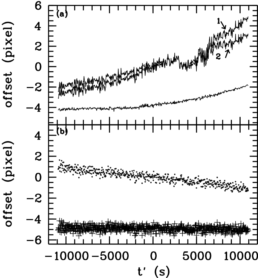
Figure 11: (a) The lowest curve (offset by 3.5 pixels) shows the pixel positions of the O i $\lambda$ 5577 Å line as a function of time. The upper curve (1) shows the variations in the position of H$\beta$ while (2) shows the variations in H$\beta$ after correcting for instrumental flexure. (b) The dots show the resulting positions of H$\beta$ after shifting with respect to H$\gamma$ and the pluses the final positions of H$\beta$ after correcting for both flexure and refraction (offset by 5 pixels). (a) and (b) together show the various stages in the processing that lead to the final positions of the lines. Note that although the above figure is for the first night only, it is representative of the procedure for both nights.

The effect of differential refraction on line and continuum intensities is non-negligible even at modest airmasses and increases rapidly with decreasing wavelength. Having corrected for instrumental flexure, the resulting positions of the Balmer lines vary linearly with $\sin\alpha\tan\zeta$ where $\alpha$ is the difference between the parallactic and position angles and $\zeta$ is the zenith distance. This is indicative of the remaining shifts being dominated by refraction. (Upper curve Fig. 11b). We computed a value for the refractive index relative to that at H$\gamma$ using the standard prescription of Stone (1996) and use this value to correct all pixels in the spectrum. As the position of the stars in the slit was altered after a correction for a guider malfunction (on the second night) compared to that at the beginning of the observing run, we applied a 5.1 Å shift to the spectra of both components. This shift was computed by measuring the wavelength of H$\gamma$ of HS 0507A in a narrow-slit (0$\aas@@fstack{\prime\prime}$7) frame and insisting that the average wavelength of H$\gamma$ – as obtained from line-profile fitting – be the same. For complete consistency, we applied a 1.74 Å shift to the spectra of the previous night.

Appendix B HS 0507A

As was mentioned in Sect. 3, the non-variability of HS 0507A is crucial to the velocity measurements and the continuum variations of HS 0507B as these are carried out with respect to HS 0507A. The measurements of HS 0507A are, of course, not carried out relative to any other star, this is further elaborated in Fig. 12.

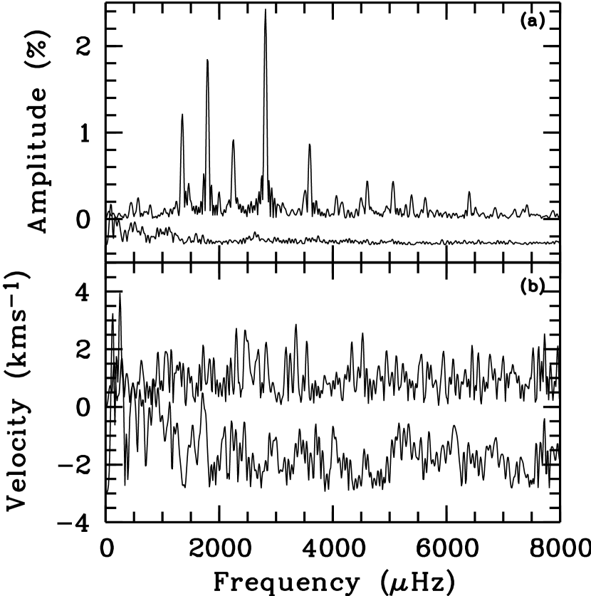
Figure 12: (a) Fourier transforms of the light curves of HS 0507B (top) and HS 0507A (offset by $-$0.3%) (b) Fourier transforms of the velocity curves of HS 0507B (top) and HS 0507A (offset by $-3$ kms^-1). The average velocity curve of HS 0507A, as used here, was constructed from the flexure and refraction-corrected positions of the three strongest Balmer lines. Polynomial fits were used to describe wandering in the slit for HS 0507A whereas H$\gamma$ of HS 0507A was used to correct for wander of HS 0507B as described in Sect. 3. The error in a single measurement of the velocities for HS 0507A is $\sim$ 9 kms^-1. Note the lack of significant velocity signal in HS 0507A at the frequency of the strongest mode as obtained from the flux variations of HS 0507B. The Fourier transforms shown here are for the first night only.