Measuring $\alpha$ in the Early Universe:
CMB Temperature, Large-Scale Structure and Fisher Matrix Analysis

Abstract

We extend our recent work on the effects of a time-varying fine-structure constant $\alpha$ in the cosmic microwave background, by providing a thorough analysis of the degeneracies between $\alpha$ and the other cosmological parameters, and discussing ways to break these with both existing and/or forthcoming data. In particular, we present the state-of-the-art CMB constraints on $\alpha$, through a combined analysis of the BOOMERanG, MAXIMA and DASI datasets. We also present a novel discussion of the constraints on $\alpha$ coming from large-scale structure observations, focusing in particular on the power spectrum from the 2dF survey. Our results are consistent with no variation in $\alpha$ from the epoch of recombination to the present day, and restrict any such variation to be less than about $4\%$. We show that the forthcoming MAP and Planck experiments will be able to break most of the currently existing degeneracies between $\alpha$ and other parameters, and measure $\alpha$ to better than percent accuracy.

I Introduction

The search for observational evidence for time or space variations of the ‘fundamental’ constants that can be measured in our four-dimensional world is an extremely exciting area of current research, with several independent claims of detections in different contexts emerging in the past year or so, together with other improved constraints Murphy et al. (2001a); Webb et al. (2001); Murphy et al. (2001b, c); Avelino et al. (2001); Fujii (2002); Ivanchik et al. (2001). We will review these in Sect. II.

Most of the current efforts have been concentrating on the fine-structure constant, $\alpha$, both due to its obviously fundamental role and due to the availability of a series of independent methods of measurement. Noteworthy among these is the Cosmic Microwave Background (CMB) Avelino et al. (2000a, b); Battye et al. (2001); Avelino et al. (2001). The latest available CMB results Avelino et al. (2001) yield a one-sigma indication of a smaller $\alpha$ in the past, but are consistent with no variation at the two-sigma level. However, these results are somewhat weakened by the existence of various important degeneracies in the data, and furthermore not everybody agrees on which and how strong these degeneracies are Avelino et al. (2000b); Battye et al. (2001); Huey et al. (2002).

Here we aim to clarify this issue by analyzing these possible degeneracies in some detail, mainly by means of a Fisher Matrix Analysis (FMA), see Sect. IV. We will emphasize that there are crucial differences between ‘theoretical’ degeneracies (due to simple physical mechanisms) and ‘experimental’ degeneracies (due to the fact that each CMB experiment only probes a limited range of scales, and that the experimental errors are scale-dependent). We will also show how such degeneracies can be eliminated either by using complementary data sets (such as large-scale structure constraints, see Sect. III) or by acquiring better data (such as that to be obtained by MAP and Planck). We present our conclusions in Sect. V.

In a companion paper Rocha et al. (2002) we will discuss a further way in which these degeneracies can be broken, namely by including information from CMB polarization.

II The Present Observational Status

The recent explosion of interest in the study of varying constants is mostly due to the results of Webb and collaborators Murphy et al. (2001a); Webb et al. (2001); Murphy et al. (2001b, c) of a $4\sigma$ detection of a fine-structure constant that was smaller in the past,

$$\frac{\Delta\alpha}{\alpha}=(-0.72\pm 0.18)\times 10^{-5}\,,\quad z\sim 0.5-3.5\,;$$ (1)

indeed, more recent work Webb (2001) provides an even stronger detection. These results are obtained through comparisons of various transitions (involving various different atoms) in the laboratory and in quasar absorption systems, using the fact that the size of the relativistic corrections goes as $(\alpha Z)^{2}$. A number of tests for possible systematic effects have been carried out, all of which have been found either not to affect the results or to make the detection even stronger if corrected for.

A somewhat analogous (though simpler) technique uses molecular hydrogen transitions in damped Lyman-$\alpha$ systems to measure the ratio of the proton and electron masses, $\mu=m_{p}/m_{e}$ (using the fact that electron vibro-rotational lines depend on the reduced mass of the molecule, and this dependence is different for different transitions). The latest results Ivanchik et al. (2001) using two systems at redshifts $z\sim 2.3$ and $z\sim 3.0$ are

$$\frac{\Delta\mu}{\mu}=(5.7\pm 3.8)\times 10^{-5}\$$ (2)

or

$$\frac{\Delta\mu}{\mu}=(12.5\pm 4.5)\times 10^{-5}\,,$$ (3)

depending on which of the (two) available tables of ‘standard’ laboratory wavelengths is used. This implies a $1.5\sigma$ detection in the more conservative case, though it also casts some doubts on the accuracy of the laboratory results, and on the influence of systematic effects in general.

We should also mention a recent re-analysis Fujii (2002) of the well-known Oklo bound Damour and Dyson (1996). Using new Samarium samples collected deeper underground (aiming to minimize contamination), these authors again provide two possible results for both $\alpha$ and the analogous coupling for the strong nuclear force, $\alpha_{s}$,

$$\frac{\dot{\alpha}}{\alpha}\sim\frac{\dot{\alpha}_{s}}{\alpha_{s}}=(0.4\pm 0.5)\times 10^{-17}yr^{-1}$$ (4)

or

$$\frac{\dot{\alpha}}{\alpha}\sim\frac{\dot{\alpha}_{s}}{\alpha_{s}}=-(4.4\pm 0.4)\times 10^{-17}yr^{-1}\,.$$ (5)

Note that these are given as rates of variation, and effectively probe timescales corresponding to a cosmological redshift of about $z\sim 0.1$. Unlike the case above, these two values correspond to two possible physical branches of the solution. See Fujii (2002) for a discussion of why this method yields two solutions (and also note that these results have opposite signs relative to previously published ones Fujii et al. (2000)). While the first of these branches provides a null result, (5) is a strong detection of an $\alpha$ that was larger at $z\sim 0.1$, that is a relative variation that is opposite to Webb’s result (1). Even though there are some hints (coming from the analysis of other Gadolinium samples) that the first branch is preferred, this is by no means settled and further analysis is required to verify it.

Still we can speculate about the possibility that the second branch turns out to be the correct one. Indeed this would definitely be the most exciting possibility. While in itself this wouldn’t contradict Webb’s results (since Oklo probes much smaller redshift and the suggested magnitude of the variation is smaller than that suggested by the quasar data), it would have striking effects on the theoretical modelling of such variations. In fact, proof that $\alpha$ was once larger than today’s value would sound the death knell for any theory which models the varying $\alpha$ through a scalar field whose behaviour is akin to that of a dilaton. Examples include Bekenstein’s theory Bekenstein (1982) or simple variations thereof Sandvik et al. (2002); Olive and Pospelov (2002). Indeed, one can quite easily see Damour and Nordtvedt (1993); Santiago et al. (1998) that in any such model having sensible cosmological parameters and obeying other standard constraints $\alpha$ must be a monotonically increasing function of time. Since these dilatonic-type models are arguably the simplest and best-motivated models for varying alpha from a particle physics point of view, any evidence against them would be extremely exciting, since it would point towards the presence of significantly different, yet undiscovered physical mechanisms.

Finally, we also mention that there have been recent proposals Braxmaier et al. (2001) of more accurate laboratory tests of the time independence of $\alpha$ and the ratio of the proton and electron masses $\mu$ using monolithic resonators, which could improve current bounds by an order of magnitude or more.

However, given that there are both theoretical and experimental reasons to expect that any recent variations will be small, it is important to develop tools allowing us to measure $\alpha$ in the early universe, as variations with respect to the present value could be much larger then.

In what follows we focus on the analysis of CMB data allowing for possible variations of the fine-structure constant. In our previous work Avelino et al. (2001), we have carried out a joint analysis using the most recent CMB (BOOMERanG and DASI) and big-bang nucleosynthesis (BBN) data, finding evidence at the one sigma level for a smaller alpha in the past (at the level of $10^{-2}$ or $10^{-3}$), though at the two sigma level the results were consistent with no variation. However, as can be seen by comparing with earlier work Avelino et al. (2000b); Battye et al. (2001) (and has also been discussed explicitly in these papers), these results are quite strongly dependent on both the observational datasets and the priors one uses.

Regarding this latter issue, we point out that a recent Coc et al. (2002) improved analysis of standard BBN (focusing mostly on nuclear physics aspects) suggests that ${}^{7}Li$ could lead to more stringent constraints on the baryonic density of the universe ($\Omega_{b}$) than deuterium. The point made by the authors is that ${}^{7}Li$ is effectively a better baryometer than $D$, because of difficulties in obtaining (extrapolated) primordial abundances of the latter. They then obtain values for $w_{b}\equiv\Omega_{b}h^{2}$ that are considerably lower than the standard ones. These results are also corroborated by Cyburt et al. (2001). Using these results as a prior would transform our previous result Avelino et al. (2001) into a detection of a varying $\alpha$ at more than two sigma.

In any case, previous analyses of CMB data allowing for a varying $\alpha$ Avelino et al. (2000b); Battye et al. (2001); Avelino et al. (2001) have revealed some interesting degeneracies between $\alpha$ and other cosmological parameters, such as $\Omega_{b}$ or $H_{0}$. On the other hand, a recent ‘brute-force’ exploration of a particular sector of parameter space (including quintessence models) Huey et al. (2002) seems to claim results on degeneracies between the various parameters Avelino et al. (2000b); Battye et al. (2001); Avelino et al. (2001).

While the two approaches are not really comparable (Huey et al. (2002) being rather more simplistic, as it uses no actual data and has somewhat unclear criteria for the presence of a degeneracy), this discrepancy begs the question of whether the degeneracies found in Avelino et al. (2000b); Battye et al. (2001); Avelino et al. (2001) are real ‘physical’ and fundamental degeneracies, which will remain at some level, no matter how much more accurate data one can get, or if they are simply degeneracies in the data, which won’t necessarily be there in other (better) datasets. And a related question is, of course, assuming that the degeneracies are significant, how can one get around them. We will address these issues in the following sections.

III Current CMB and Large-Scale Structure Constraints

Here we present an up-to-date analysis of the Cosmic Microwave Background constraints on varying $\alpha$ as well as, for the first time, an analysis of its effects on the large-scale structure (LSS) power spectrum.

Even though this may not be entirely obvious, a varying $\alpha$ will have an effect on the matter power spectrum. The simplest way to understand this is to interpret the variation in $\alpha$ as being due to a variation in the speed of light $c$ (which one is always free to do Avelino and Martins (1999)).

A variation in $\alpha$ affects the matter power spectrum to the extent that it changes the horizon size, hence the turnover scale in the matter power spectrum. Allowing for a variation in $\alpha$, this is not only a function of $\Omega_{m}$, $\Omega_{B}$ and $h$ but of $\alpha$ as well, through the dependence of the recombination epoch on $\alpha$. Therefore varying alpha will produce a change in the turnover point position $k_{rec}$ of the matter power spectrum, hence a shift of the curve sideways, and therefore a change on the value of $\sigma_{8}$. For example a decrease in $\alpha$ shifts this turnover scale to smaller $k$, hence allowing for a decrease in $\sigma_{8}$.

By plotting the transfer functions (generated with a modified Avelino et al. (2000b) version of the CMBFAST Seljak and Zaldarriaga (1996) code which includes the effects of a varying $\alpha$) we find that this effect is fairly small. For $\Omega_{m}=0.3$ and $\Omega_{B}=0.05$ and keeping all other cosmological parameters fixed a variation of $\alpha$ by say $10\%$ from its standard value produces variations in the transfer function which are at most $5\%$ in restricted regions of $k$ (the effect on the value of $\sigma_{8}$ is even smaller).

On the other hand a change in $\alpha$ will modify the height of the first peak of the CMB power spectrum through the (early) ISW effect. This effect also depends on $\Omega_{m}h^{2}$. This illustrates the interplay between a varying $\alpha$, $\Omega_{m}$ and the value of $\sigma_{8}$. Further effects of a varying $\alpha$ in the CMB are a slight change in the position of the first peak due to the aforementioned change in the horizon size, plus a variation in the high-$\ell$ damping (due to the finite thickness of the last-scattering surface) which are also dependent on a number of cosmological parameters other than $\alpha$.

It should be emphasized that although these CMB and LSS constraints are in some sense complementary, and can help break degeneracies by determining other cosmological parameters, they certainly can not be blindly combined together, since the range of cosmological epochs (or redshifts) to which they are sensitive is somewhat different.

III.1 CMB data analysis

We compare the recent CMB observations with a set of flat models with parameters sampled as follows (the value in brackets is the step size):

$$\Omega_{m}=0.1\ldots(0.1)\ldots 1.0$$ (6)

$$\Omega_{b}=\Omega_{m}-\Omega_{cdm}=0.009\ldots(0.003)\ldots 0.036$$ (7)

$$\frac{\Delta\alpha}{\alpha}=0.80\ldots(0.01)\ldots 1.10$$ (8)

$$h=0.40\ldots(0.05)\ldots 0.90$$ (9)

$$n_{s}=0.70\ldots(0.05)\ldots 1.30\,.$$ (10)

We rescale the amplitude of fluctuations by a pre-factor $C_{10}$, in units of $C_{10}^{COBE}$, with $0.50<C_{10}<1.40$. Finally, we assumed a negligible re-ionization and an optical depth $\tau_{c}\sim 0$. This is in agreement with recent estimates on the redshift of re-ionization $z_{re}\sim 6\pm 1$ (see e.g. Gnedin (2001)).

The theoretical models are computed using a modified version of the publicly available CMBFAST program Seljak and Zaldarriaga (1996), accounting for the effects of a varying $\alpha$, and are compared with the recent BOOMERanG-98, DASI and MAXIMA-1 results. The power spectra from these experiments were estimated in $19$, $9$ and $13$ bins respectively, spanning the range $25\leq\ell\leq 1150$.

For the DASI and MAXIMA-I experiment we use the publicly available correlation matrices and window functions. For the BOOMERanG experiment we assign a constant value for the spectrum in each bin $\ell(\ell+1)C_{\ell}/2\pi=C_{B}$, we approximate the signal $C_{B}$ inside the bin to be a Gaussian variable and we consider $\sim 10\%$ correlations between contiguous bins. The likelihood for a given cosmological model is then defined by

$$-2{\rm ln}{\cal L}=(C_{B}^{th}-C_{B}^{ex})M_{BB^{\prime}}(C_{B^{\prime}}^{th}-C_{B^{\prime}}^{ex})\,,$$ (11)

where $M_{BB^{\prime}}$ is the Gaussian curvature of the likelihood matrix at the peak. We consider $10\%$, $4\%$ and $5\%$ Gaussian distributed calibration errors for the BOOMERanG-98, DASI and MAXIMA-1 experiments respectively and we included the beam uncertainties by the analytical marginalization method presented in Bridle et al. (2001). We also include the COBE data using Lloyd Knox’s RADPack packages.

III.2 LSS data analysis

In what follows, we will add to the CMB data the real-space power spectrum of galaxies in the 2dF 100k galaxy redshift survey using the data and window functions of the analysis of Tegmark et al. (2001).

To compute ${\cal L}^{2dF}$ we, evaluate $p_{i}=P(k_{i})$, where $P(k)$ is the theoretical matter power spectrum and $k_{i}$ are the $49$ k-values of the measurements in Tegmark et al. (2001). Therefore we have

$$-2ln{\cal L}^{2dF}=\sum_{i}[P_{i}-(Wp)_{i}]^{2}/dP_{i}^{2}\,,$$ (12)

where $P_{i}$ and $dP_{i}$ are the measurements and error bars in Tegmark et al. (2001) and $W$ is the reported $27\times 49$ window matrix. We restricted the analysis to a range of scales where the fluctuations are assumed to be in the linear regime ($k<0.02h^{-1}Mpc$). When combining with the CMB data, we marginalize over a bias $b$ considered as additional free parameter.

We will also include information on $\sigma_{8}$, the RMS mass fluctuation in spheres of $8h^{-1}Mpc$, obtained from local cluster number counts. There is presently no consensus on the correct value of this observable, mainly because of systematics in the calibration between cluster virial mass and temperature. For convenience of analysis, we consider $2$ values: an high value $\sim\Omega_{m}^{0.6}\sigma_{8}=0.50\pm 0.05$ in agreement with the results of Pierpaoli et al. (2001); Eke et al. (1996) and a lower one, $\sim\Omega_{m}^{0.6}\sigma_{8}=0.40\pm 0.05$ following the analysis of Seljak (2001); Viana et al. (2001).

We attribute a likelihood to each value of $\delta\alpha/\alpha$ by marginalizing over the nuisance parameters. We then define our $68\%$ ($95\%$), confidence levels to be where the integral of the likelihood is $0.16$ ($0.025$) and $0.84$ ($0.975$) of the total value (see e.g. Melchiorri et al. (2000)).

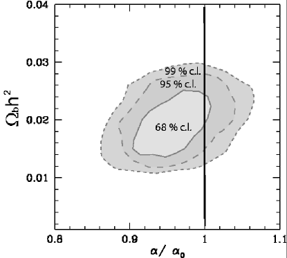
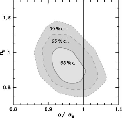
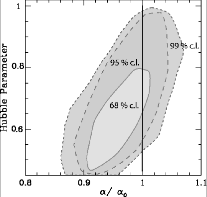
Figure 1: The current combined CMB constraints on the $\omega_{b}-\alpha/\alpha_{0}$, $n_{s}-\alpha/\alpha_{0}$ and $h-\alpha/\alpha_{0}$ planes.

Table 1: Current cosmological constraints on the variation of the fine-structure constant (marginalizing over other parameters) for various different priors.

Prior	$\alpha/\alpha_{0}$ (95 % c.l.)
$h=0.65\pm 0.2$	$0.95_{-0.06}^{+0.07}$
BBN $\omega_{b}=0.02\pm 0.002$	$0.96_{-0.05}^{+0.06}$
HST $h=0.71\pm 0.08$	$0.98_{-0.05}^{+0.05}$
SN-Ia	$0.95_{-0.06}^{+0.07}$
$\Omega_{m}^{0.6}\sigma_{8}=0.50\pm 0.05$	$1.01_{-0.04}^{+0.04}$
$\Omega_{m}^{0.6}\sigma_{8}=0.40\pm 0.05$	$0.99_{-0.05}^{+0.05}$
2dF	$0.98_{-0.05}^{+0.04}$

III.3 Results

In a previous work Avelino et al. (2001) we produced likelihood contours in the $\Omega_{b}h^{2}-\alpha/\alpha_{0}$ plane by analyzing the recent BOOMERanG and DASI CMB datasets and by including two priors to the analysis: flatness and $h=0.65\pm 0.2$. Our results were consistent with the baryon abundance obtained from big-bang nucleosynthesis (BBN) and we constrained variations in $\alpha$ at $z\sim 1000$ at level of about $10\%$. In Fig. 1 we plot constraints on this plane, as well as on the $n_{s}-\alpha/\alpha_{0}$ and $h-\alpha/\alpha_{0}$ planes with a similar analysis, but including this time the MAXIMA-I dataset.

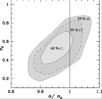
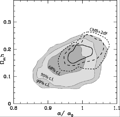
Figure 2: The current combined CMB constraints on the $\sigma_{8}-\alpha/\alpha_{0}$ and $\Omega_{m}h-\alpha/\alpha_{0}$ planes. The latter panel also shows the results of combining the CMB and 2dF datasets.

From these results we can see that the inclusion of the MAXIMA-I data doesn’t significantly change our previous constraints. In fact, even if the analysis of the MAXIMA-I data alone suggests a higher value of the baryon fraction ($\Omega_{b}h^{2}\sim 0.030\pm 0.005$ Stompor (2001)), the combined analysis with DASI and BOOMERanG still suggests a low value of $\Omega_{b}h^{2}\sim 0.023$. This result is in agreement with previous analysis, e.g. Tegmark et al. (2001).

From last two panels of Fig. 1 we also see that, in the set of models we are considering, there is a clear correlation between variations in $\alpha$ and changes in the scalar spectral index $n_{s}$ and the Hubble parameter $h$. We will see in the next section that this degeneracy can be broken by the future and more accurate measurements from satellite experiments like MAP MAP (2002) or the Planck Surveyor Planck (2002).

However, since variations in $n_{s}$ and $h$ affect the shape, position and amplitude of the matter power spectrum (irrespective of changes in $\alpha$), we can in principle use the data from galaxy clustering and local cluster abundances in order to break these degeneracies and infer stronger constraints on $\alpha$. Regarding the RMS amplitude of mass fluctuations on scales of $8h^{-1}Mpc$, the two effects are competitive: an increase in $n_{S}$ will increase $\sigma_{8}$, while lowering $h$ decreases it. As we can see from the first panel of Fig. 2, the effect from $h$ is stronger and the final result is that a decrease in $\alpha$ generally allows for lower amplitudes of $\sigma_{8}$.

Furthermore, as we can see from Fig. 2, a certain degree of degeneracy is present in the CMB data between $\alpha$ and the shape parameter $\Omega_{m}h$. This degeneracy can be optimally broken by incorporating the data from the 2dF galaxy survey. As we can see in the bottom panel, including the 2dF data shrinks the contours around $\alpha/\alpha_{0}\sim 1$ and $\Omega_{m}h\sim 0.2$, In other words, there is a clear distinction between the CMB and LSS data: while for the CMB data a negative variation of $\alpha$ is preferred, the opposite happens for the LSS data. When the two datasets are combined, the best-fit model, in the $\Omega_{m}h-\alpha/\alpha_{0}$ plane, is quite close to the standard one.

We should emphasize at this point that in doing this we are not combining direct constraints on the parameter $\alpha$ itself, obtained through both methods, to obtain a tighter constraint. As mentioned above this can not be done, since the CMB and LSS analyses are sensitive to the values of $\alpha$ at different redshift ranges, so there is no reason why these values should be the same. Additionally, there is no well-motivated theory that could relate such variations at different cosmological epochs. All that one could do at this stage would be to assume some toy model where a certain behaviour would occur, but this would mean introducing various additional parameters, thus weakening the analysis. Hence we chose not to pursue this path and leave the analysis as model-independent as possible.

What we are doing is using additional information (which is also sensitive to $\alpha$) to better constrain other parameters in the underlying cosmological model, such as $n_{s}$, $h$ and the densities of various matter components, which we can reliably assume are unchanged throughout the cosmological epochs in question. In other words, we are simply selecting more stringent priors for our analysis, in a self-consistent way.

The constraints obtained by combined analysis are reported in Table 1. Our main result from this table is that, as one would expect, when constraints from other and independent cosmological datasets are included in the CMB analysis, the constraints on variations on $\alpha$ become significantly stronger.

IV Fisher Matrix Analysis

The precision with which the forthcoming satellite experiments MAP MAP (2002) and Planck Planck (2002) will be able to determine variations in $\alpha$ can be readily estimated with a Fisher Matrix Analysis (FMA). Some authors have already performed such an analysis in the past Hannestad (1999); Kaplinghat et al. (1999): however, their analysis was based on a different set of cosmological parameters and assumed cosmic variance limited measurements. In our FMA we also take into account the expected performance of the MAP and Planck satellites and we make use of a cosmological parameters set which is well adapted for limiting numerical inaccuracies. Furthermore, the FMA can provide useful insight into the degeneracies among different parameters, with minimal computational effort.

IV.1 Analysis Setup

We characterize the cosmological model by a 7 dimensional parameter set, given by

$${\bf\Theta}=(\alpha,\omega_{b},\omega_{m},\omega_{\Lambda},{\mathcal{R}},n_{s},Q),$$ (13)

where $\omega_{b}\equiv\Omega_{b}h^{2}$ is the physical baryonic density, $\omega_{m}\equiv(\Omega_{\rm cdm}+\Omega_{b})h^{2}$ the energy density in matter and $\omega_{\Lambda}$ the energy density due to a cosmological constant. Here $h$ denotes the Hubble parameter today, $H_{0}\equiv 100h$ km s^-1 Mpc^-1. The quantity ${\mathcal{R}}\equiv\ell_{\rm ref}/\ell$ is the ‘shift’ parameter (see Melchiorri and Griffiths (2001); Bowen et al. (2001) and references therein), which gives the position of the acoustic peaks with respect to a flat, $\Omega_{\Lambda}=0$ reference model, $n_{s}$ is the scalar spectral index and $Q=<\ell(\ell+1)C_{\ell}>^{1/2}$ denotes the overall normalization, where the mean is taken over the multipole range $2\leq\ell\leq 2000$.

The shift parameter ${\mathcal{R}}$ depends on $\Omega_{m}$, on the curvature $\Omega_{\kappa}\equiv 1-\Omega_{\Lambda}-\Omega_{m}-\Omega_{\rm rad}$ through

$${\mathcal{R}} = 2\left(1-\frac{1}{\sqrt{1+z_{\rm dec}}}\right)$$ (14)

$$\times\frac{\sqrt{|\Omega_{\kappa}|}}{\Omega_{m}}\frac{1}{\chi(y)}\left[\sqrt{\Omega_{\rm rad}+\frac{\Omega_{m}}{1+z_{\rm dec}}}-\sqrt{\Omega_{\rm rad}}\right],$$

where $z_{\rm dec}$ is the redshift of decoupling, $\Omega_{\rm rad}$ is the energy parameter due to radiation ($\Omega_{\rm rad}=4.13\cdot 10^{-5}/h^{2}$ for photons and 3 neutrinos) and

$$y = \sqrt{|\Omega_{\kappa}|}\int_{0}^{z_{\rm dec}}\,dz$$

$${[\Omega_{\rm rad}(1+z)^{4}+\Omega_{m}(1+z)^{3}+\Omega_{\kappa}(1+z)^{2}+\Omega_{\Lambda}]^{-1/2}}.$$

The function $\chi(y)$ depends on the curvature of the universe and is $y$, $\sin(y)$ or $\sinh(y)$ for flat, closed or open models, respectively. Inclusion of the shift parameter ${\mathcal{R}}$ into our set of parameters takes into account the geometrical degeneracy between $\omega_{\Lambda}$ and $\omega_{m}$ Efstathiou (2001). With our choice of the parameter set, ${\mathcal{R}}$ is an independent variable, while the Hubble parameter $h$ becomes a dependent one.

We assume throughout purely adiabatic initial conditions and we do not allow for a tensor contribution. In the FM approach, the likelihood distribution for the parameters $\bf\Theta$ is expanded to quadratic order around its maximum. We denote this maximum likelihood (ML) point by $\bf\Theta_{0}$ and call the corresponding model our “ML model”, with parameters $\omega_{b}=0.0200$ (hence $\Omega_{b}=0.0473$), $\omega_{m}=0.1267$ (hence $\Omega_{m}=0.3000$), $\omega_{\Lambda}=0.2957$ (hence $\Omega_{\Lambda}=0.7000$ and $h=0.65$), ${\mathcal{R}}=0.9628$, $n_{s}=1.00$, $Q=1.00$. For the value of $z_{\rm dec}$ in eq. (IV.1)(which is weakly dependent on $\omega_{b}$ and $\omega_{\rm tot}$) we have used the fitting formula from Hu and Sugiyama (1995). For the ML model we have $z_{\rm dec}=1115.52$.

Table 2: Experimental parameters for MAP and Planck (nominal mission). Note that the sensitivities are here expressed in $\mu$K.

	MAP			Planck
$\nu$ (GHz)	$41$	$61$	$95$	$100$	$143$	$217$
$\theta_{c}$ (arcmin)	$31.8$	$21.0$	$13.8$	$10.7$	$8.0$	$5.5$
$\sigma_{c}$ ($\mu$K)	$19.8$	$30.0$	$45.6$	$4.6$	$5.4$	$11.7$
$w^{-1}_{c}\cdot 10^{15}$ (K2 ster)	$33.6$	$33.6$	$33.6$	$0.215$	$0.158$	$0.350$
$\ell_{c}$	$254$	$385$	$586$	$757$	$1012$	$1472$
$\ell_{\rm max}$	$1000$			$2000$
$f_{\rm sky}$	$0.80$			$0.80$

Proceeding as described in Bowen et al. (2001), we then calculate the Fisher information matrix

$$F_{ij}=\sum_{\ell=2}^{\ell_{\rm max}}\frac{1}{\Delta C_{\ell}^{2}}\frac{\partial C_{\ell}}{\partial\Theta_{i}}\frac{\partial C_{\ell}}{\partial\Theta_{j}}|_{\bf\Theta_{0}}$$ (16)

The quantity $\Delta C_{\ell}$ is the standard deviation on the estimate of $C_{\ell}$:

$$\Delta C_{\ell}^{2}=\frac{2}{(2\ell+1)f_{\rm sky}}(C_{\ell}+{B}_{\ell}^{-2})^{2}.$$ (17)

The first term is the cosmic variance, arising from the fact that we exchange ensemble average with a spatial average. The second term takes into account the expected error of the experimental apparatus Knox (1995); Efstathiou (2001):

$${B}_{\ell}^{2}=\sum_{c}w_{c}e^{-\ell(\ell+1)/\ell_{c}^{2}}\,.$$ (18)

The sum runs over all channels of the experiment, with the inverse weight per solid angle $w_{c}^{-1}\equiv(\sigma_{c}\theta_{c})^{-2}$ and $\ell_{c}\equiv\sqrt{8\ln 2}/\theta_{c}$, where $\sigma_{c}$ is the sensitivity (in $\mu$K) and $\theta_{c}$ is the FWHM of the beam (assuming a Gaussian profile) for each channel. Furthermore we can neglect the issues arising from point sources, foreground removal and galactic plane contamination assuming that once they have been taken into account we are left with a “clean” fraction of the sky given by $f_{\rm sky}$.

The experimental parameters are summarized in Table 2. We use the 3 higher frequency MAP channels and the first 3 channels of the Planck High Frequency Instrument (HFI). Adding the 3 higher frequency channels of the HFI and the 3 channels of Planck’s Low Frequency Instrument leaves the expected errors unchanged: therefore they can be used for foreground removal, consistency checks, etc, leaving the HFI channels for cosmological use.

For Gaussian fluctuations, the covariance matrix is then given by the inverse of the Fisher matrix, $C=F^{-1}$ Bond et al. (1999). The $1\sigma$ error on the parameter $\Theta_{i}$ with all other parameters marginalised is then given by $\sqrt{C_{ii}}$. If all other parameters are held fixed to their ML values, the standard deviation on parameter $\Theta_{i}$ reduces to $\sqrt{1/F_{ii}}$ (conditional value). Other cases, in which some of the parameters are held fixed and others are being marginalized over can easily be worked out.

A case of interest is the one in which all parameters are being estimated jointly: then the joint error on parameter $i$ is given by the projection on the $i$-th coordinate axis of the 7-dimensional hyper-ellipse which contains a fraction $\gamma$ of the joint likelihood. The equation of the hyper-ellipse is

$$({\bf\Theta-\Theta_{0}}){\bf F}({\bf\Theta-\Theta_{0}})^{t}=q_{1-\gamma},$$ (19)

where $q_{1-\gamma}$ is the quantile for the probability $1-\gamma$ for a $\chi^{2}$ distribution with 7 degrees of freedom. For $\gamma=0.683$ ($1\sigma$ c.l.) we have $q_{1-\gamma}=8.18$.

The FMA assumes that we are expanding the likelihood function at the right point, ie that the parameters values of the true model are in the vicinity of ${\bf\Theta_{0}}$. The validity of the results depends on this assumption, as well as on the assumption that the $a_{\ell m}$’s are independent Gaussian random variables. If the FM predicted errors are small enough, the method is self-consistent and we can expect the FM prediction to reproduce in a correct way the exact behaviour. This is indeed the case for the present analysis, with the notable exception of $\omega_{\Lambda}$, which suffers from the geometrical degeneracy (see next section).

Special care must be taken in computing the derivatives of the power spectrum with respect to the cosmological parameters. Numerical errors in the spectra can lead to larger derivatives, which would artificially break degeneracies among parameters. In the present work we implement double–sided derivatives, which diminish the truncation error from second order to third order terms. The choice of the step size is a trade-off between truncation error and numerical inaccuracy dominated cases. For an estimated numerical precision of the computed models of order $10^{-4}$, the step size should be approximately 5% of the parameter value Press et al. (1992). It turns out that for derivatives in direction $\alpha$ and $n_{s}$ the step size can be chosen to be as small as $0.1\%$. As for the other parameters, the accuracy is limited by the fact that differentiating around a flat model requires computing open and closed models, which are calculated using different numerical techniques. The relative numerical noise is therefore much larger. After several tests, we chose step sizes varying from $1\%$ to $5\%$ for $\omega_{b},\omega_{m},\omega_{\Lambda}$, and ${\mathcal{R}}$. This choice gives derivatives with an accuracy of about $0.5\%$. The derivatives with respect to $Q$ are exact, being the power spectrum itself.

IV.2 Analysis results

IV.2.1 FMA forecast

Table 3 summarizes the results of our FMA. MAP will be able to constrain variations in $\alpha$ at the time of last scattering to within $2\%$ ($1\sigma$, all others marginalised). This corresponds to an improvement of a factor of 3 relative to the limits presented in the previous section. Planck will narrow it down to about half a percent. If all other parameters are supposed to be known and fixed to their ML value, then a factor of 10 is to be gained in the accuracy of $\alpha$ (compare the columns labelled “fixed” in table 3). However, if all parameters are being estimated jointly, the accuracy on variations in $\alpha$ will not go beyond $1\%$, even for Planck (column “joint”).

The parameters $\omega_{b},{\mathcal{R}}$ and $n_{s}$ suffer from partial degeneracies with $\alpha$, which are discussed in more detail in the next section. This is only partially reflected in the marginalized errors of table 3. Correlations among the parameters play an important role: within the limit of the quadratic order approximation, they are fully described by the FM.

The geometrical degeneracy limits the accuracy on $\omega_{m}$ and $\omega_{\Lambda}$. The degeneracy is so severe that the error on $\omega_{\Lambda}$ is very unsensitive to the experimental details. From the FMA point of view, this happens because the derivative of the spectrum with respect to $\omega_{\Lambda}$ vanishes for $\ell\gtrsim 50$. Therefore probing higher multipoles does not help for the purpose of better constraining the cosmological constant. We emphasize once more that such a large error cannot be trusted to be accurate in any respect: it just signals a very large inaccuracy in $\omega_{\Lambda}$. The errors on all other parameters, however, are small enough to justify the self-consistency of the FMA approach.

Table 3: Fisher matrix analysis results: expected $1\sigma$ errors for the MAP and Planck satellites. The column marg. gives the error with all other parameters being marginalized over; in the column fixed the other parameters are held fixed at their ML value; in the column joint all parameters are being estimated jointly.

Quantity	$1\sigma$ errors (%)
	MAP			Planck HFI
	marg.	fixed	joint	marg.	fixed	joint
$\alpha$	2.24	0.13	6.39	0.41	0.02	1.16
$\omega_{b}$	5.11	1.12	14.61	0.98	0.31	2.79
$\omega_{m}$	5.26	1.97	15.04	2.30	0.44	6.59
$\omega_{\Lambda}$	97.81	89.62	279.74	95.17	89.55	272.18
${\mathcal{R}}$	3.73	0.20	10.67	0.57	0.03	1.64
$n_{s}$	1.79	0.52	5.12	1.19	0.13	3.42
$Q$	1.19	0.36	3.41	0.19	0.10	0.54

The power of an experiment can be roughly assessed by looking at the eigenvalues $\lambda_{i}$ and eigenvectors ${\bf u^{(i)}}$ of its FM: the error along the direction in parameter space defined by ${\bf u^{(i)}}$ (principal direction) is proportional to $\lambda_{i}^{-1/2}$. But we are interested in determining the errors on the physical parameters rather then on their linear combinations along the principal directions. Therefore in the ideal case we want the principal directions to be as much aligned as possible to the coordinate system defined by the physical parameters. We display in Table 4 eigenvalues and eigenvectors of the FM for MAP and Planck. Planck’s errors, as measured by the inverse square root of the eigenvalues, are smaller by a factor of about 4 on average. For 6 of the 7 eigenvectors Planck also obtains a better alignment of the principal directions with the axis of the physical parameters. This is established by comparing the ratios between the largest (marked with an asterisk in Table 4) and the second largest (marked with a dagger) cosmological parameters’ contribution to the principal directions. This is of course in a slightly different form the statement that Planck will measure the cosmological parameters with less correlations among them.

Table 4: In the lines we display the components of the eigenvectors of the FM for MAP and Planck. The quantity $1/\sqrt{\lambda_{i}}$ is proportional to the error along the principal direction ${\bf u^{(i)}}$. For each principal direction, an asterisk marks the largest cosmological parameters contribution, a dagger the second largest. Not only Planck has errors smaller by a factor of about 4 on average, but also the alignment of the principal directions with the axis defined by the physical parameter is better than MAP in 6 cases out of 7.

MAP
Direction $i$	$1/\sqrt{\lambda_{i}}$	$\omega_{b}$	$\omega_{m}$	$\omega_{\Lambda}$	$n_{s}$	$Q$	${\mathcal{R}}$	$\alpha$
1	2.23E-04	9.9540E-01*	-9.7492E-03	-1.8938E-05	-1.6970E-02	-4.2258E-03	-6.8163E-02${\dagger}$	6.4257E-02
2	1.12E-03	-7.8215E-02	2.8225E-01	1.6168E-05	1.6425E-01	-1.4652E-01	-4.4305E-01${\dagger}$	8.1822E-01*
3	2.43E-03	4.0471E-02	7.2825E-01*	2.0996E-04	1.4674E-01	-5.6711E-01${\dagger}$	2.6310E-01	-2.3590E-01
4	8.63E-03	3.9968E-03	6.1138E-01${\dagger}$	8.1457E-03	-3.7196E-01	6.4228E-01*	-2.3162E-01	-1.4702E-01
5	4.45E-02	-1.9844E-02	-6.8856E-02	-1.6683E-02	2.5892E-01	-1.8786E-01	-8.0247E-01*	-4.9829E-01${\dagger}$
6	1.38E-02	3.1792E-02	1.0650E-01	-1.5423E-02	8.6336E-01*	4.5726E-01${\dagger}$	1.7932E-01	-2.8026E-02
7	2.89E-01	2.0351E-04	-4.6453E-03	9.9971E-01*	2.0638E-02${\dagger}$	-1.1925E-03	-8.7876E-03	-7.5125E-03
Planck
Direction $i$	$1/\sqrt{\lambda_{i}}$	$\omega_{b}$	$\omega_{m}$	$\omega_{\Lambda}$	$n_{s}$	$Q$	${\mathcal{R}}$	$\alpha$
1	5.81E-05	9.3678E-01*	8.2153E-03	-1.2417E-06	9.2222E-03	3.0060E-03	-1.8611E-01	2.9604E-01${\dagger}$
2	2.87E-04	-3.2830E-01	2.5649E-01	9.3971E-06	1.5805E-01	2.0156E-01	-3.8542E-01${\dagger}$	7.8248E-01*
3	5.46E-04	1.1323E-01	8.4059E-01*	4.5325E-06	2.7521E-01	2.5135E-01	3.2628E-01${\dagger}$	-1.8765E-01
4	1.94E-03	3.8999E-02	-3.1741E-01${\dagger}$	-9.3635E-05	-3.8346E-02	9.4091E-01*	6.4234E-02	-8.2576E-02
5	2.86E-03	-1.5404E-02	2.9918E-01	7.3411E-04	-3.9324E-01	9.9942E-02	-7.5339E-01*	-4.2194E-01${\dagger}$
6	1.30E-02	8.7278E-03	-1.9309E-01	-1.6271E-02	8.6190E-01*	-2.9783E-02	-3.7230E-01${\dagger}$	-2.8285E-01
7	2.81E-01	1.6073E-04	-3.3978E-03	9.9987E-01*	1.4308E-02${\dagger}$	-4.7295E-04	-5.4974E-03	-4.3069E-03

IV.2.2 Degeneracies with other parameters

In previous work Avelino et al. (2000b) some of the present authors observed a degeneracy in the Boomerang-98 and Maxima-1 data between $\alpha$ and $\omega_{b}$. This degeneracy also shows up in the present analysis (see Fig. 1, top panel). The question we ask is: is this a fundamental degeneracy, or is it only in the data?

Figure 3: Ellipses containing $68\%$ ($1\sigma$) of joint confidence (all other parameters marginalized) in the $\alpha/\alpha_{0}-\omega_{b}$, $\alpha/\alpha_{0}-n_{s}$ and $\alpha/\alpha_{0}-{\mathcal{R}}$ planes for the FM simulated Boomerang, MAP and Planck.

We have performed a FMA with experimental parameters chosen as to mimic a Boomerang-type experiment ($f_{\rm sky}=0.02,\sigma=15\quad\mu\rm{K},\theta=9.2^{\prime},\ell_{\rm max}=1000$). If the degeneracy is due to the limited precision of the present-day experimental data, we expect the degeneracy to disappear as we move from Boomerang, to MAP, to Planck. Fig. 3 (top panel) shows $1\sigma$ joint confidence curves (all other parameters marginalized) in the $\alpha/\alpha_{0}-\omega_{b}$ plane for the FM simulated Boomerang, MAP and Planck (from the outside to the center, respectively). The curve for Boomerang is to be compared with the $1\sigma$ contour of the data analysis (Figure 1, top panel). Although the FM ellipse is centred by construction at the ML model value, it is in qualitative agreement with the result of the data analysis. As we move to MAP, the degeneracy shrinks but is still there: only higher multipole measurements from Planck can break it.

The same behaviour is observed in the $\alpha/\alpha_{0}-n_{s}$ plane (Fig. 3, middle panel; compare with Fig. 1, middle panel). Again, the observed degeneracy between $\alpha$ and $n_{s}$ is clearly revealed by the FMA for Boomerang.

In the bottom panel of Fig. 3 we investigate the important degeneracy between ${\mathcal{R}}$ and $\alpha/\alpha_{0}$. These two parameters are very highly correlated (correlation $\approx 0.99$ for all experiments), because an increase of $\alpha$ displaces the acoustic peaks to higher multipoles. This effect is mainly due to the increased redshift of last scattering Kaplinghat et al. (1999); Avelino et al. (2000b). On the contrary, an increase of ${\mathcal{R}}$ shifts the peaks toward smaller $\ell$ values, because of the change in the angular diameter distance relation. However, an increase in $\alpha$ also produces a decrease in the damping at high multipoles, which can be used to break the degeneracy, as it is the case for Planck. This is reflected in the different amplitude for the two derivatives, which are otherwise perfectly in phase, as can be seen in Fig. 4. This degeneracy can clearly be identified because of our choice of the parameter set ${\bf\Theta}$, which includes the shift parameter rather than the Hubble or curvature parameters. This emphasizes the importance of a correct choice of the parameter set in the context of a FMA.

Comparison to previous works is only partially possible, because of the differences in the analysis discussed above. Our detailed analysis confirms however the conclusions in refs. Hannestad (1999); Kaplinghat et al. (1999), which found that a cosmic variance limited experiment could obtain a precision on $\alpha$ of order $10^{-3}-10^{-2}$. We have also shown that there is much to be gained from using prior knowledge about the other parameters in the determination of $\alpha$ via CMB measurements. The improvement in accuracy is about a factor $50$ for both MAP and Planck.

Figure 4: Derivatives with respect to $\alpha$ and ${\mathcal{R}}$. We plot $-\partial C_{\ell}/\partial\alpha$ to facilitate the comparison with $\partial C_{\ell}/\partial{\mathcal{R}}$. The two derivatives are perfectly in phase: this is responsible for the degeneracy between the corresponding parameters. Only the different amplitudes allow an experiment which maps sufficiently high multipoles with high accuracy to distinguish between them.

V Conclusions

We have provided an up-to-date analysis of the effects of a varying fine-structure constant $\alpha$ in the CMB, focusing on the issue of the degeneracies with other cosmological parameters, and of how these can be broken.

We have shown that the currently available data is consistent with no variation of $\alpha$ from the epoch of recombination to the present day, though interestingly enough the CMB and LSS datasets seem to prefer, on their own, variations of $\alpha$ with opposite signs. Whether or not this statement has any physical relevance (beyond the results of the statistical analysis) is something that remains to be investigated in more detail. In any case, any such (relative) variation is constrained to be less than about $4\%$, so a best-fit or ‘concordance’ model with $\alpha$ exactly constant will require, at most, some slight deviations of other cosmological parameters from the ‘standard’ values obtained from analyses which don’t allow for $\alpha$ variation.

On the other hand, the prospects for the future are definitely bright. In the short term, the imminent VSA and CBI data should be able to provide some improvement on the current results. The dataset we have used (BOOMERanG, MAXIMA and DASI) all have the common feature that their error bars are smallest for data points around the first Doppler peak and larger for smallest angular scales. Now, as we have explicitly shown above (and was already suggested in Avelino et al. (2000b)), the first Doppler peak is not a vary accurate ‘$\alpha$-meter’, due to the degeneracy with the shift parameter. Thus datasets in which points around the first peak will somewhat dominate the statistical analysis are not optimal for $\alpha$ estimation. In this regard, VSA and CBI should be useful because they can provide a significant number of data points on small angular scales with relatively small error bars, hence minimizing this problem.

In the longer term, the forthcoming satellite experiments will provide a dramatic improvement on these results. We have performed a Fisher Matrix Analysis using a well adapted parameter set and realistic experimental characteristics for the upcoming MAP and Planck satellite missions. The results of our forecast are that MAP and Planck will be able to constrain variations in $\alpha$ within $2.2\%$ and $0.4\%$, respectively ($1\sigma$ c.l., all other parameters marginalized). If all parameters are being estimated simultaneously, then this limits increase to about $6.4\%$ and $1.1\%$, respectively. The analysis of the presently observed degeneracies between $\alpha$ and $\omega_{b}$, $n_{s}$ comes to the conclusion that measurement of higher multipoles will allow to break it. We have also identified an important degeneracy between $\alpha$ and the shift parameter.

To conclude, we have provided a thorough analysis of the effects of cosmological parameter degeneracies in CMB measurements of the fine-structure constant $\alpha$, and quantified the importance of these degeneracies. We have also explicitly discussed two ways in which these degeneracies can be circumvented, namely acquiring better data (the easy solution, at least from the theorists’ point of view) or combining the CMB data with other cosmological datasets which can provide constraints on other cosmological parameters (the ‘brute-force’ solution)

In a follow-up paper, we will discuss a third way in which these degeneracies can be lifted, namely including CMB polarization data Rocha et al. (2002) (the more elegant solution in principle, though it’s yet to be realized in practice). These tools, together with other measurements coming from BBN Avelino et al. (2000b) and quasar and related data Murphy et al. (2001a); Webb et al. (2001) offer the exciting prospect of being able to map the value of $\alpha$ at very many different cosmological epochs, which would allow us to impose very tight constraints on higher-dimensional models where these variations are ubiquitous.