Mass Composition of Cosmic Rays in the Range
$2\times 10^{17}-3\times 10^{18}$ eV Measured with the Haverah Park Array

Abstract

At the Haverah Park Array a number of air shower observables were measured that are relevant to the determination of the mass composition of cosmic rays. In this paper we discuss measurements of the risetime of signals in large area water-Cherenkov detectors and of the lateral distribution function of the water-Cherenkov signal. The former are used to demonstrate that the CORSIKA code, using the QGSJET98 model, gives an adequate description of the data with a low sensitivity, in this energy range, to assumptions about primary mass. By contrast the lateral distribution is sufficiently well measured that there is mass sensitivity. We argue that in the range 0.2–1.0 EeV the data are well represented with a bi-modal composition of $(34\pm 2)$% protons and the rest iron. We also discuss the systematic errors induced by the choice of hadronic model.

1 Introduction

High-energy cosmic rays are measured via extensive air showers of secondary particles they produce in the Earth’s atmosphere. Specific observables depend in a complex way on primary mass and energy, which must be understood to interpret air shower data. Some measurable parameters at ground can be used to obtain the primary energy of the incoming cosmic rays without large systematic uncertainties due to the unknown composition [1]. The main effect of a variable mass on showers with the same initial energy, $E$, is a characteristic shift of the position of the maximum of shower development in the atmosphere, $X_{\rm m}$. Cosmic ray nuclei share their energy amongst $A$ nucleons and, therefore, their showers can, to a first approximation, be described as a superposition of $A$ nucleon-induced subshowers with an energy of $E/A$ each. Thus, showers of heavy primaries are less penetrating, and tend to develop higher up in the atmosphere, than nucleon showers of the same energy. Therefore, $X_{\rm m}$ is an observable with a strong connection to the primary mass. However, additionally, the depth of maximum also depends on energy. The higher the energy the longer the shower and the deeper is $X_{\rm m}$. This is described by the elongation rate, d$X_{\rm m}$/d$\log E$, which is usually quoted as the shift in $X_{\rm m}$ per change of energy by a factor 10. In practice, apart from the unique case of fluorescence detectors, there is no way to measure $X_{\rm m}$ directly. Mostly other quantities are recorded that can be shown to have a correlation to the height of the shower development.

Here we report an analysis of mass composition in the energy range 0.2–1.0 EeV that has been performed with data from the Haverah Park extensive air shower array. The Haverah Park array was a 12 km² air shower array consisting of water tanks that acted as Cherenkov detectors. It was operational from 1967 to 1987.

At Haverah Park a number of observables were measured which are relevant to the determination of the mass composition of cosmic rays above $2\times 10^{17}$ eV. In particular, the two parameters, $\eta$ and t_1/2, which are sensitive to the longitudinal development of showers, have been studied in detail. $\eta$ describes the steepness of the lateral distribution function of the signal observed in the water-Cherenkov detectors. $\eta$ was measured with high precision using a portion of the array with a much denser detector arrangement, the so-called infill array [2]. For 1425 events in the energy range $2\times 10^{17}$ to $3\times 10^{18}$ eV information from infill detectors was available and $\eta$ could be determined. These were recorded between 1977 and 1981.

Figure 1: The inner part of the Haverah Park array, the so called infill array.

The second mass-sensitive parameter, the risetime t_1/2, is a measure characterising the spread of the arrival times of individual particles at a given detector. It is evaluated from the integrated signal of all particles belonging to a shower and defines the time interval in which the integrated signal rises from 10% to 50%. Risetimes can be sensibly determined only in large-area detectors. Therefore they are obtained from the four 34 m² detectors, A1–A4 (Fig. 1). Risetime data were obtained from $>7000$ events and a total of 13000 detector signals at core distances of more than 300 m. The events used here span a range of energies from $2\times 10^{17}$ to $2\times 10^{19}$ eV.

The analysis of risetimes of events with known core position, arrival direction and energy established the first evidence of shower-to-shower fluctuations at high energies [3]. This was supported by the demonstration of a correlation of t_1/2 with the steepness of the lateral distribution, which could be understood as a consequence of both variables being dependent on $X_{\rm m}$. In the 1970s and 1980s it was not possible to make accurate predictions of the t_1/2 expected for different primary masses because the problem could not be solved analytically and a full 4-dimensional numerical simulation was beyond the capabilities of the computing power accessible at that time.

The analysis of $\eta$ data also showed evidence of fluctuations very much larger than could be attributed to the experimental uncertainties [4]. The dependence of $\eta$ on the depth of the shower development in the atmosphere could not be established directly from the data. Furthermore, a comparison of the measured average value of $\eta$ with a highly regarded model calculation of the time [5] showed strikingly poor agreement: a mean cosmic-ray mass very much heavier than iron was required to fit the data (see Fig. 2).

Figure 2: A comparison of Haverah Park data and the calculations for p and Fe induced showers from [5]. $\rho$ is the water-Cherenkov signal.

The situation is now very different and a model can be found that describes the data rather well. To interpret the data detailed simulations with the CORSIKA and GEANT programs have been performed. CORSIKA [6] is a modern air shower model that simulates particle production and propagation in the atmosphere fully. It employs various models of high-energy hadronic interactions, of which the most tested is QGSJET98 (Quark-Gluon-String model with jets) [7]. The GEANT program [8] is used to account for the detector response to particles of different type, energy and impact angle.

2 The Haverah Park Array

The Haverah Park array has been described in detail elsewhere [9]. The central part of the array is composed of four 34 m² water-Cherenkov detectors, A1–A4, spaced 500 m apart. Six groups of satellite arrays each of 4 $\times$ 14 m² lie near to a circumference of radius 2 km around the centre so that density information is available from all sites for showers that trigger the 500 m array. The 500 m array is sensitive to showers with primary energies above $\approx 6\times 10^{16}$ eV. Another set of three detectors (9 m² each) surrounding the central detector (A1) form a 150 m array. The so-called infill array consists of 23 small-area water-Cherenkov detectors located in the central region of the 500 m array with an irregular spacing of $\approx 150$ m. For the arrangement of detectors, see Fig. 1. Further small-area detectors were placed right next to the 9 m² detectors and A1 for calibration purposes.

There were two kind of detectors: (i) 2.29 m² area galvanized rectangular iron tanks with aluminum lids, identical to those used in the 4 $\times$ 34 m² detectors: these detectors were placed inside wooden huts with light roofs, and (ii) 1 m² area water tanks, made of light-weight polyurethane foam and covered with fibre glass: these tanks of hexagonal cross section, stood outdoors. All tanks were filled with water to a depth of 1.2 m and viewed by one photomultiplier with 100 cm² photocathode. Detector areas larger than 2.29 m² were achieved by grouping several of the 2.29 m² detectors together. Sixteen of the modules form each of the detectors A1–A4. The signals from 15 of the 16 tanks were summed to provide the signal used for triggering and for the density estimate. The 16^th tank in each group was used to provide a low gain signal. 4 modules make up the 9 m² detectors and 6 modules form the 13 m² detectors.

The densities of Cherenkov photons per unit detector area (Cherenkov densities) were recorded in terms of the average signal from a vertical muon (1 vertical equivalent muon = 1 vem) per square metre. This signal corresponds to approximately 14 photoelectrons (pe) for Haverah Park tanks. A trigger for all detectors is generated when the central detector (A1) and at least two out of the three other A-sites (A2, A3, A4) detect a particle density of $>0.3$ vem/m². However, infill signals had to be above 7 vem/m² to be recorded. Trigger rates were monitored daily over the life of the experiment. After correction for atmospheric pressure variations, the trigger rates were found to be stable to better than 5%.

A feature of the Haverah Park array, which is particularly important for the shower front measurements, is the area of the detectors A1–A4. These detectors allow large samples of the shower front to be taken at widely separated points, thus minimizing the chance of observing effects due only to local density fluctuations. The temporal response of the recording system to a step function was determined by measuring the response to small showers that fell nearby and thus produced short risetimes. The risetime of bandwidth limited pulses was 45 ns [10].

Cross-calibration of the detectors of the infilled array with the other detectors could have been achieved using vertical muons, as for the large-area detectors, so that they yield the same response to a purely muonic signal. However with such a cross-calibration one would have had to correct for the different response of the detectors to the soft component and for differences in optical and geometrical properties of the detectors and so an alternative approach was adopted. Signals from individual 2.29 m² and 1 m² detectors, next to A1, were compared with corresponding densities from the 34 m² detector, and an appropriate conversion factor was obtained. Similar calibration procedures were used on simulated data for consistency.

3 Model calculations

At present the CORSIKA program is effectively the standard tool for air shower simulations, and it is successfully used by a variety of different experiments over the energy range from 1–10¹² GeV. CORSIKA uses EGS4 (Electron Gamma Shower code) [11] for the simulation of the electromagnetic interactions, and features a detailed simulation of particle propagation and decay. However, most important for the development of air showers in the atmosphere are soft hadronic interactions. At present the only available theoretical approach to model these is Gribov-Regge theory of multi-Pomeron exchange. Several interaction models based on this theory are available in CORSIKA, the most successful being QGSJET [7]. The QGSJET model also contains the treatment of hard collisions and the production of mini-jets, which become dominant at very high energy collisions, and includes a realistic simulations of nucleus-nucleus collisions. Its parameters were tuned to fit a wide range of accelerator results and to provide a secure extrapolation to the highest energies. The combination of CORSIKA with QGSJET seems to be able to describe experimental cosmic ray results from Cherenkov telescopes at $10^{12}$ eV [12], over measurements of the hadronic, muonic and electromagnetic shower components in the knee region [13], to lateral distributions and arrival times as will be shown in this work, up to air showers at $10^{20}$ eV [14].

Using the CORSIKA code with QGSJET98 we have generated a library of proton and iron showers with zenith angles: $0^{\circ}$, $15^{\circ}$, $26^{\circ}$, $40^{\circ}$ and $45^{\circ}$ at a primary energy of $4~{}\times~{}10^{17}$ eV, and for a zenith angle of $26^{\circ}$ at energies of 0.2, 0.4, 0.8, 1.6, and 3.2 EeV. For each set 100 showers with the same parameters have been simulated. Additionally we have generated sets of 100 showers with oxygen and helium primaries at zenith angle 26^∘ and energy 0.4 EeV. In total 3600 showers were produced. Statistical thinning of shower particles was applied at the level of 10${}^{-6}\times$ E with a maximum particle weight limit of 10${}^{-13}\times$ E/eV.

Predictions of the risetimes were deduced from the time information of each individual particle contained in the simulated shower library. The time distribution of the signals produced by electromagnetic particles for different core distances ($r$) was obtained for each simulated shower. The integral over the distribution was normalized to the expected signal from electromagnetic particles at the given distance for a 34 m² detector. The arrival time distribution of muons has been obtained for different $r$. The expected number of muons at a given $r$ for a 34 m² detector has been computed and Poisson fluctuations added. The muons are sampled from the arrival time distribution to obtain the time distribution of the muon signal in the detector. The time distributions of the muon signal and the soft component were then added and convoluted with the known system response to an instantaneous pulse. The risetime is then inferred from the result of the convolution. This procedure was repeated 100 times for each shower to get the mean risetime as a function of $r$ and the expected spread of the risetimes arising from Poisson fluctuations in the number of muons. To increase the statistics further each CORSIKA shower was thrown 100 times onto the array with random core positions ranging out to 300 m from the centre of the array. The risetime at each of the four 34 m² detectors is calculated from the parameterisations obtained above. The risetime at each detector is smeared according to an error that contains contributions from Poisson fluctuations in the number of muons and from the experimental measurement error ($\approx$ 3 ns). The core distance of each detector was varied according to the error in the core position described in [1]. To reproduce the multiplicity of measured risetimes per event in the data, we keep only the core position and the risetime of some of the detectors. We repeated this procedure for each of the 100 CORSIKA showers in a set and the mean risetime versus $r$ is obtained (Fig. 3).

To obtain a value of $\eta$ for each simulated shower we have convoluted the CORSIKA output with the detector response and fitted the resulting lateral distribution function for muons and electromagnetic particles. Again, each shower was used 100 times with core positions randomly scattered over the infilled area, obtaining the densities at each detector with the parameterisations described above. The densities are modified according to Poisson fluctuations in the number of particles. We tested whether an event meets the array trigger conditions and, if so, the densities were fluctuated according to measurement errors and recorded in the same format as real data. The calibration of the infilled array is reproduced with simulations to obtain the conversion factor described in the previous section. To obtain the energy of the showers, either simulated or real, we need its relation to the water-Cherenkov signal density at a core distance of 600 m, $\rho(600)$, and the attenuation length $\lambda$. The procedure to calculate these is described in ref. [1]. Here we have followed the same procedure. The uncertainty in the core position, for the $\eta$ analysis, is $\approx 5$ m for all energies and primary masses tested. The energy resolution for proton primaries falls from 15% at 0.4 EeV to 10% at 6.4 EeV, while for iron primaries it is 10% and 7%, respectively. These uncertainties include physical fluctuations in $\rho(600)$ and measurement errors.

4 Risetime analysis

Figure 3: Risetime versus distance to shower core as obtained in data and in simulations for proton and iron primaries.

The dependence of the risetime of the signal in a detector on shower development arises largely because of geometry. Particle scattering, velocity differences and geomagnetic deflections are second order effects: the geometrical sensitivity is enhanced at large distances. The set of nuclear interactions that produce particles observed at an off-axis detector may be regarded as lying on a line source. There are two important properties of this line source that relate to mass composition and affect the observed risetime. These are its position in the atmosphere and its length.

Previous studies of t_1/2 have revealed its dependence on $\theta$, energy and core distance, and used deviations from mean values as measures of the variations of $X_{\rm m}$ with energy to get results on mass composition. The variations deduced [15] were in good accord with measurements made subsequently and directly by the Fly’s Eye group [16].

The strategy for the present analysis is different: the risetime as a function of core distance for different bins of $\theta$ and $E$ are compared directly with predictions from Monte Carlo simulations for different primary masses. In the energy and distance ranges ($250<r<500$ m) of interest here, where $\eta$ has been obtained with high accuracy, the sensitivity of the risetime technique for the extraction of mass information is rather limited. The technique is, however, expected to be very effective for mass separation at greater distances and in larger showers where the mean risetime difference predicted between proton and iron showers is large and easy to measure. The results of such a study will be described elsewhere. At small distances limitations of bandwidth mean that relatively large samples of showers were required to establish the dependence of risetime on energy and zenith angle and to demonstrate shower-to-shower fluctuations [15, 3]. However this relative insensitivity to mass can be turned to advantage by using the data to test whether a shower model is able to predict average risetimes accurately over the distance range discussed here. In Fig. 3 we compare the mean risetime with distance, for two zenith angle bands, with model predictions. The data lie between the predictions for protons and iron: it is not wise to deduce any mass information from these plots because of known systematic uncertainties in the data and the models at the few nanosecond level. The flattening-off evident at the smaller core distances is a consequence of the low bandwidth of the 1970s recording system.

Two cuts were applied to the data and to the simulation results to obtain Fig. 3: the density in a particular detector had to be greater that 1 vem/m² (to reduce sampling fluctuations), and the position of the core had to be closer than 300 m from the central triggering detector (to avoid large core errors).

We infer from this analysis that the CORSIKA code, using QGSJET98 physics, gives a very adequate description of the mean shower risetime as a function of distance from 200–800 m and over the zenith angle range 15^∘–40^∘. This is the first time that such agreement has been demonstrated. While the comparisons of Fig. 3 do not provide proof that the QGSJET98 model is correct they do give us reasonable confidence in using this model to attempt to interpret other data that are expected to show mass sensitivity.

5 Lateral distribution analysis

5.1 Event reconstruction

First the shower direction was determined using the arrival time information of the four central triggering detectors. The particle density information was then analysed to find the shower core. The lateral distribution, parameterised with respect to the known core position and the primary energy, is estimated from the particle densities and the form of the lateral distribution using the correlation between $\rho(600)$ and energy. At a given energy the lateral distribution was found to be well described experimentally by the modified power law:

$$\rho(r)=k~{}r^{-(\eta+r/4000~{}{\rm m})}\\$$ (1)

and fits well to the average data in the distance range 80–800 m. $\eta$ was shown to vary with zenith angle as $\eta=3.78-1.44~{}\sec\theta$.

Due to the small number of densities usually available without the infill array, it was not possible to fit reliably values of $\eta$ for each individual shower. Therefore, the dependence of $\eta$ on zenith angle was obtained by calculating the average water-Cherenkov lateral distribution function for different zenith angle bins. However, the great number of densities available with the infill array allows study of the fluctuations of the lateral distribution on a shower-by-shower basis.

The original algorithm used to determine the shower parameters is described as follows. For a given lateral distribution function geometrical reconstruction provides a unique core location using only a small number of density measurements. For each selected event the core was found using 3 or 4 detectors surrounding the probable core position. The geometrical mean distance of the shower core from these “ringing” detectors was in the range $50<r_{\rm n}<200$ m. Only densities at distances $>r_{\rm n}$ were used to determine the lateral distribution function using a $\chi^{2}$ minimisation technique. An iterative procedure was used to find the best value of $\eta$ for each event using as a starting point the energy independent approximation of $\eta$ given above. A multiple linear regression was used to determine the dependence of $\eta$ [17] on zenith angle and energy. The result was

$$\eta=a-b\,(\sec\theta-1)+c\log(E/10^{17}{\rm eV})$$

with $a=2.20\pm 0.01$, $b=1.29\pm 0.05$, and $c=0.165\pm 0.022$. The difficulty of the ringing analysis is the implementation of the algorithm. The optimum set of ringing detectors was chosen subjectively. Several factors were considered in the choice of ringing analysis but the experience of the observer was also important. For the purposes of this analysis, in which a large statistical sample of simulated events is generated to compare with data, another technique described below was adopted to find the optimum shower parameters, so that the role of the observer was removed.

The algorithm used here is a grid search over many different core position. For a given core position the best value of $\eta$ and $k$ are found through an analytical fit and the $\chi^{2}$ function is computed. We used only detector densities above threshold and below saturation in the range 80–800 m. Densities above saturation and below threshold do not improve the fit because of the large number of recorded densities available in this data set. Fig. 4 shows an example of a reconstructed event using this method and the ringing analysis. The difference in the value of $\eta$ between the two analyses were found to be $\approx 0.08$, which agrees with the measurement error reconstruction in $\eta$ for the two techniques ($\approx 0.08$).

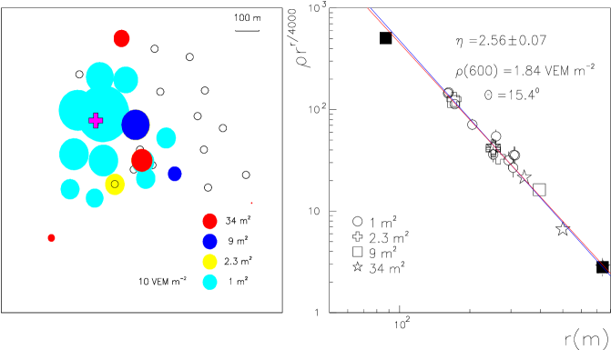
Figure 4: Example of the reconstruction of an infill event. Left panel: Projection of the array into the shower plane with recorded densities shown as circles with radius proportional to the logarithm of the density. The detector areas are indicated by grey scales. The detectors are displayed in the plane perpendicular to the shower axis. Right panel: Fitted lateral distribution function. The two lines correspond to the lateral distribution function as obtained with ringing analysis and with the method described in the text. The difference in the value of $\eta$ for this particular event is 0.04. The abscissa shows a quantity that linearises the lateral distribution function given in Eq. 1. Filled symbols indicate detectors with signals above saturation or below threshold.

The selection criteria applied to the data are the following:

• Zenith angles in the range 0^∘–45^∘.

• In every shower the core must be located within the infilled area.

• Showers in which the largest density is at one of the boundary detectors are excluded.

• The value of $\chi^{2}$ from the $\eta$ fitting procedure should correspond to the “goodness of the fit” having a probability greater than 1%.

After the application of these criteria 1351 showers remain from the initial number of 1450. This is the data set we use to compare with model calculations.

5.2 Model comparison

We use two independent methods to extract information about mass composition from the lateral distribution function. The first one is based on the $\chi^{2}$ method and the second one on the likelihood approach. The first technique is more direct and allows a visual check of the procedure, but requires the use of zenith angle cuts in our data set, reducing thus the statistics. The second method allows us to combine all the zenith angles to predict the mass composition in different energy ranges. We will show that the two methods are consistent but we will give our final results in terms of the second method.

5.2.1 Method 1

The simulated events generated from CORSIKA showers are analysed with the same algorithms as real data and the same cuts are applied. In Fig. 5(a) the variation of $\eta$ with zenith angle is shown for events with energies in the range 0.3–0.5 EeV. It is evident that, if the mean mass lies between the limits of proton and iron, the lower energy data are well described by the QGSJET98 model.

In Fig. 5(b) and 6 we show the variation of $\eta$ with energy. In Fig. 5(b) data in three zenith angle ranges are displayed. The model calculations shown for the four mass species are for the boundary between the two most vertical zenith angle bands. In Fig. 6 the data have been normalised to $26^{\circ}$ for comparison with calculations at the same angle. The agreement between the normalised data and a smaller data set in the range $1.06<\sec\theta<1.16$ is good and gives confidence in the normalisation procedure. A linear fit to the normalised data is shown: the reduced $\chi^{2}$ is 1.1. The data might be described with a single mass component, independent of energy, or by a mixture of several mass components. To distinguish between these possibilities we use data on the spread of $\eta$.

Figure 5: Right panel: evolution of $\eta$ with zenith angle; the simulation results correspond to a zenith angle of 26^∘, the data is binned in zenith angle bands. Left panel: evolution of $\eta$ with zenith angle for data and simulations.

Figure 6: Evolution of $\eta$ with energy for data and simulation results.

Figure 7: Distributions of $\eta$ for experimental data, and model predictions with different primary masses.

Although the average properties of showers do not vary strongly with primary mass, fluctuations in the longitudinal development are substantially larger for proton than for iron-initiated showers. The smaller fluctuations for nucleus-induced showers is a direct consequence of the superposition of A nucleonic showers, produced after the initial nucleus fragments, which tends to average out extreme fluctuations that might occur in individual subshowers. To study fluctuations in $\eta$, two $\eta$ distribution were constructed: (i) showers with 1.06$<\sec\theta<1.16$ and 0.2 EeV$<E<0.6$ EeV (292 events), and (ii) showers with $1.04<\sec\theta<1.18$ and 0.6 EeV$<E<1.0$ EeV (46 events).

To compare with simulations, we account for all sources that could contribute to the spread of $\eta$, namely fluctuations in the longitudinal development of the shower and reconstruction errors. These are automatically taken into account, since fluctuations are contained in the simulated event sample, and the same reconstruction methods are used for simulated events as for real ones. The typically root mean square spread from “shower-to-shower fluctuations” is 0.12 for proton showers and 0.05 for iron showers, and from the measurement error in $\eta$ is $\approx$ 0.08.

In Fig. 7(a) and (b) the experimental data in the energy band 0.2–0.6 EeV are compared with predictions for proton and iron beams. The reduced $\chi^{2}$ for the fits are 31 and 6.4, respectively. The tail at large $\eta$ in the comparison with iron indicates that some light nuclei are required to fit the measurements. For helium and oxygen the corresponding $\chi^{2}$ values are 20.0 and 7.0. A fit to a dual component mixture is shown in Fig. 7(c). A mixture with ($29\pm 4$)% of protons and a corresponding amount of iron is a very good fit ($\chi^{2}/{\rm dof}=1.04$): the addition of small amounts of helium and oxygen ($<2$%) gives $\chi^{2}/{\rm dof}=0.8$. In Fig. 7(d) we show 46 events in the energy range 0.6–1.0 EeV and zenith angle range $1.04<\sec\theta<1.18$: a two component fit gives ($30\pm 10$)% protons.

We thus conclude that there is no evidence for any change of mass with energy in the range studied and that Fe is the dominant component. The data of Fig. 6 do not exclude the possibility of the Fe component getting larger as the energy reaches 1 EeV and then smaller beyond.

5.2.2 Method 2

The zenith angle cuts used in the procedure described above do not allow us to use all the data available in a given energy range to extract mass composition. For this reason we have developed an additional technique, using the likelihood method, that exploits the data more effectively.

For each set of CORSIKA showers at a given energy and zenith angle we have generated an $\eta$ distribution. Each set consists of 100 CORSIKA showers, and each shower was thrown randomly onto the array. We have reconstructed it with the same procedure as for the data, obtaining an $\eta$ distribution that includes the effect of shower-to-shower fluctuations and experimental reconstruction. We have fitted each resulting $\eta$ distribution to a Gaussian obtaining the mean $\mu_{\eta}$ and width $\sigma_{\eta}$.

We can parameterise the values of $\mu_{\eta}$ and $\sigma_{\eta}$ as a function of zenith angle at a fixed energy (0.4 EeV), and as a function of the energy at a fixed zenith angle (26^∘), for proton and iron primaries. Fig. 8 and 9 show these fits, which are very satisfactory. Therefore we can predict the values of these parameters for any energy and zenith angle.

The values of $\mu_{\eta}$ and $\sigma_{\eta}$ are given by:

$$\mu_{\eta}(\theta,E) = a_{1}+a_{2}~{}\Delta_{\theta}+a_{3}~{}\Delta_{\theta}^{2}+a_{4}~{}\log_{10}(E/0.4{\rm EeV})$$ (2)

$$\sigma_{\eta}(\theta,E,p) = b_{1}+b_{2}~{}\Delta_{\theta}+b_{3}~{}\log_{10}(E/0.4{\rm EeV})$$ (3)

$$\sigma_{\eta}(\theta,E,Fe) = b_{1}+b_{2}~{}\Delta_{\theta}+b_{3}~{}\exp(b_{4}~{}\log_{10}(E/0.4{\rm EeV}))$$ (4)

with $\Delta_{\theta}=\sec\theta-\sec 26^{\circ}$, and the constants obtained from the fits shown in Figs. 8 and 9 for proton and iron primaries are given in Table 1. It should be noticed that we use a different functional form for $\sigma_{\eta}$ depending on the primary. $\sigma_{\eta}$ is decreasing with increasing energy as the shower-to-shower fluctuations are reduced, but it cannot have a value smaller than the reconstruction error of $\eta$ ($\approx 0.08$), which is constant with energy. This is the reason for the flattening of the value of $\sigma_{\eta}$ for iron primaries at high energies in Fig. 9.

$\mu_{\eta}$	$a_{1}$	$a_{2}$	$a_{3}$	$a_{4}$
p	2.38 $\pm$ 0.01	-1.00 $\pm$ 0.10	-2.8 $\pm$ 0.6	0.12 $\pm$ 0.02
Fe	2.10 $\pm$ 0.01	-1.33 $\pm$ 0.06	-1.2 $\pm$ 0.3	0.19 $\pm$ 0.01
$\sigma_{\eta}$	$b_{1}$	$b_{2}$	$b_{3}$	$b_{4}$
p	0.16$\pm$ 0.01	0.25 $\pm$ 0.07	-0.03 $\pm$ 0.02	—
Fe	0.06$\pm$ 0.01	0.08 $\pm$ 0.04	0.03 $\pm$ 0.01	-2.4 $\pm$ 1.1

Table 1: Parameters obtained in the fits of Eqs. 2–4 to simulation results.

Figure 8: Variation of $\mu_{\eta}$ and $\sigma_{\eta}$ with zenith angle for proton and iron primaries at an energy of 0.4 EeV. The lines have the form of Eqs. 2–4, and are fitted to the results obtained from simulations. The top lines correspond to proton primaries and the bottom lines to iron primaries.

Figure 9: Variation of $\mu_{\eta}$ and $\sigma_{\eta}$ with primary energy for proton and iron primaries at a zenith angle of 26^∘. The lines have the form of Eqs. 2–4, and are fitted to the results obtained from simulations.

The probability density of an event to belong to a proton or iron $\eta$ distribution is given by the appropriate Gaussians:

$$G=\frac{1}{\sqrt{2\pi}\sigma_{\eta}(\theta_{i},E_{i})}\exp(-\frac{(\eta_{i}-\mu_{\eta}(\theta_{i},E_{i}))^{2}}{2\sigma_{\eta}(\theta_{i},E_{i})^{2}})\\$$ (5)

where $\theta_{i}$, $E_{i}$ and $\eta_{i}$ are the zenith angle, the energy and the reconstructed values of $\eta$ of each event.

To fit the composition, assuming only two components as seems reasonable from the discussion in 5.2.1, we use the the maximum likelihood method. The quantity to maximise in this method is:

$$\ln~{}P(F_{\rm p})=\ln(P_{1}~{}P_{2}~{}....~{}P_{n})=\sum_{i=1}^{n}~{}\ln~{}P_{i}\,,$$ (6)

where $P_{i}$ is given by:

$$P_{i}=F_{\rm p}G_{\rm p}+(1-F_{\rm p})G_{\rm Fe}$$ (7)

where $F_{\rm p}$ is the fraction of protons and $G_{\rm p}$ ($G_{\rm Fe}$) is the probability of the event to be proton (iron), as given in Eq. 5.

With this procedure we can use events at all zenith angles to fit $F_{\rm p}$ in a given energy range. As a demonstration of reliability of the method, we have divided our set of data into bins of zenith angle, selecting events between 0.3–0.5 EeV. For each angular bin we fitted the composition using the method described above. Fig. 10 shows the results. As expected, the values derived of $F_{\rm p}$ obtained do not depend on zenith angle. The average value is in agreement with the value obtained in the previous section (F${}_{\rm p}=0.30\pm 0.04$).

Figure 10: Predicted value of $F_{\rm p}$ in the energy range 0.3–0.5 EeV for different zenith angle bins. The predicted value of $F_{\rm p}$ does not depend on zenith angle.

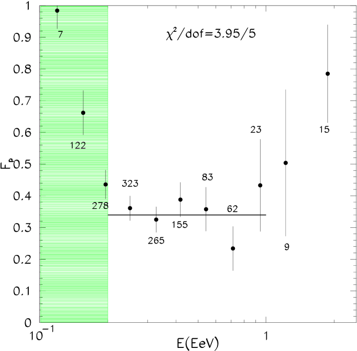
Figure 11: Predicted value of $F_{\rm p}$ as a function of the energy. A fit to a constant composition in the energy range 0.2–1.0 EeV is also shown with its corresponding $\chi^{2}$. The number of events in each energy bin is shown. The shadow region corresponds to the energy range in which the analysis is affected by trigger biases (see text).

Figure 12: Likelihood curves in two energy bands of Fig. 11. The horizontal lines correspond to a value of the maximum of the log-likelihood function minus 0.5 (1 $\sigma$ level).

We have also investigated the possibility of having oxygen and helium in the cosmic ray beam. For this purpose we have selected events in the energy range 0.3–0.5 EeV and with 1.1 $<\sec~{}\theta<1.14$ , and, using a modification of Eq. 6, fitted the fraction of oxygen (helium) assuming a three component mixture of primaries: proton, iron, and oxygen (helium). The fitted fraction of oxygen or helium are less than 1%. At 68% confidence level the fraction of oxygen (helium) should be less than 15% (25%). Therefore, as in the previous section, we will assume a dual component mixture of proton and iron for our final discussion.

Fig. 11 shows the predicted fraction of protons in the cosmic ray beam as a function of the energy. In this case we have used the events from all zenith angles. It is apparent that in the energy range 0.2–1.0 EeV the composition does not change within the limits of measurement. The rapid increase of $F_{\rm p}$ at energies below 0.2 EeV is an artificial effect. It was established very early [18] that below 0.2 EeV steep showers have a higher probability to trigger the array, and as the average proton shower is steeper than the average iron shower, $F_{\rm p}$ increases rapidly at lower energies. A fit to a constant composition in the energy range 0.2–1.0 EeV gives a predicted value of $F_{\rm p}=0.34\pm 0.02$. Examples of the likelihood curves used to extract mass composition are shown in Fig. 12 for two energy bins of Fig. 11.

We thus conclude that there is no evidence for any change of mass with energy in the range studied and that Fe is the dominant component in this energy range. The data of Fig. 11 do not exclude the possibility of the proton component being enhanced at energies larger than 1.0 EeV.

5.3 Sensitivity to hadronic model

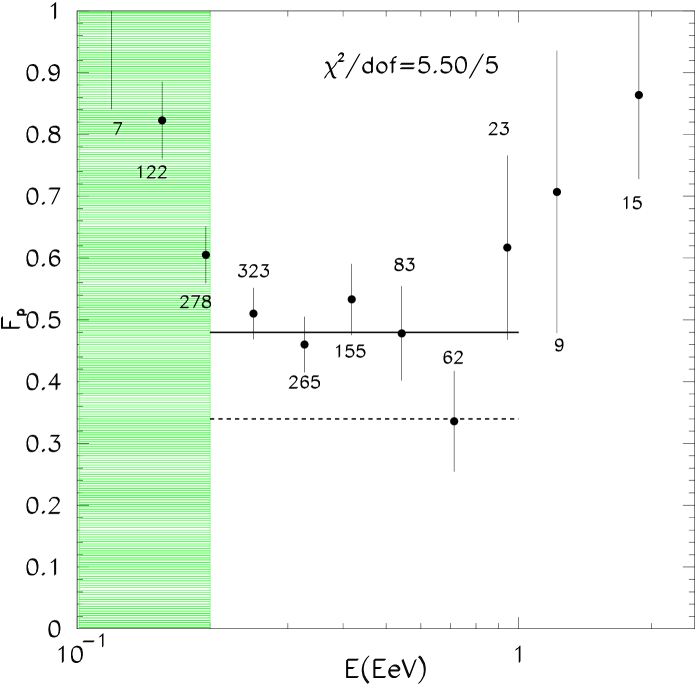
Figure 13: Predicted value of $F_{\rm p}$ as a function of the energy for QGSJET01 (solid line) and QGSJET98 (dashed line). The shadow region corresponds to the energy range in which the analysis is affected by trigger biases (see text).

The simulations presented in this work were obtained using CORSIKA and QGSJET98 as high energy interaction model. Recently QGSJET98 has been replaced by QGSJET01. The major change was a modification in the treatment of diffractive processes [19]. This change reduced the value of the position of the shower maximum $X_{\rm m}$ by $\approx$ 10 g/cm², that is showers develop higher in the atmosphere.

To establish the sensitivity of our results to this change in the hadronic model we simulated 4 sets of 100 CORSIKA showers with the new model for proton and iron primaries at a zenith angle of $26^{\circ}$ and with primary energies of 0.4, and 0.8 EeV. We found that the spread of $\eta$ ($\sigma_{\eta}$) does not change, but the value $\mu_{\eta}$ is reduced by 0.04 for both proton and iron. Therefore, we can calculate the predicted value of $F_{\rm p}$ as a function of the energy using the likelihood method, but reducing the value of $\mu_{\eta}$ in Eq. 2 by 0.04. Fig. 13 shows the results compared with the expectation obtained in the previous subsection. The value of $F_{\rm p}$ is increased from 0.34 to 0.48.

The QGSJET01 model has been shown to have the smallest value of $X_{\rm m}$ when compared to a variety of hadronic models (neXus 2, SIBYLL 2.1, DPMJET II.5) [19]. Some of these models have the mean value of $X_{\rm m}$ increased by $\approx$ 10 g/cm² compared to QGSJET98. Assuming that the ratio of electromagnetic to muonic particles in the shower for these models is the same than QGSJET98, we can estimate the changes in our results in the manner used for the QGSJET01 model. The value $\mu_{\eta}$ is now increased by 0.04 and the value of $F_{\rm p}$ is reduced from 0.34 (QGSJET98) to 0.23.

We can also estimate the changes in the risetime analysis when using another hadronic model. Using the relationship between X_m and t_1/2 in [15], a shift of $X_{\rm m}$ by $\approx$ 10 g/cm² corresponds to a change in t_1/2 at 400 m from the shower core of less than 1 ns. Hence, the agreement between data and simulations exemplified by Fig. 3 still holds.

As a final result, we state that the data on lateral distributions in the energy range 0.2–1.0 EeV is well fitted by a dual p/Fe composition with about (34 $\pm$ 2)% of the signal being protons constant in this energy range. The error in this quantity comes from the statistics of the data available. The systematic uncertainty, introduced by the choice of hadronic models, is $\approx$ 14%, larger than the statistical error. Clearly, further calculations, using a range of models, are highly desirable.

6 Comparison with other experiments and conclusions

The Haverah Park data, in the light of new hadronic models have provided a new estimation on the mass composition in the energy range 0.2–1.0 EeV. Efforts to understand the origin of cosmic rays at any energy are greatly hampered by our lack of knowledge of the mass distribution in the incoming cosmic ray beam. We have obtained here a prediction for the mass composition in the energy range 0.2–1.0 EeV. We can compare only with one experiment operating in the same energy range: the HiRes prototype, operated with the MIA detector. Using the QGSJET98 model they find a rapid change towards a light composition between 0.1–1.0 EeV [20], which is in contradiction with our results. The question of mass composition is thus far from being resolved and there is clearly scope for alternative approaches.

Some years ago an analysis of the Fly’s Eye data [21] pointed to a change from an iron dominated composition at $3\times 10^{17}$ eV to a proton-dominated composition near 10¹⁹ eV. This conclusion was drawn from a study of the variation of depth of maximum with energy (the elongation rate) and from an analysis of the spread in depth of maximum at a given energy. The conclusions on mass composition from the study of the spread in depth of maximum were confirmed by [22] but none of these analyses extended to energies above 10¹⁹ eV. A different conclusion has been reached by the AGASA group based on the variation of the muon content of showers with energy [14]. Their analysis favours a composition that remains “mixed” over the 10¹⁸ to 10¹⁹ eV decade. The statistics in this energy range from this data set are too small to be able to claim any agreement with either of the two experiments. We are starting to work on a risetime analysis in this energy range which could provide some relevant information.

We can also compare our results with the mass composition obtained by KASCADE. The mean value of the mass at their highest accessible energy ($\approx 10^{17}$ eV) was estimated to be $\langle\ln~{}A\rangle=3.5\pm 0.5$ [23], which should be compared with the result obtained in this work which corresponds to $\langle\ln~{}A\rangle=2.65\pm 0.08\pm 0.6$ in the energy range 2–10 $\times 10^{17}$ eV. In contrast to our results KASCADE also claims that protons have largely disappeared at $10^{16}$ eV.

Acknowledgments:

Thanks are given to members of the Haverah Park group who helped to get the data discussed here over 20 years ago. In particular the major contributions made by R.J.O. Reid, R.N. Coy and C.D. England are gratefully acknowledged. We are grateful to the staff of the Computing Centre of IN2P3 in Lyon and to M. Risse for the help in producing the simulated showers for this analysis.

References

- [1] Ave M. et al., The Energy Spectrum of Cosmic Rays Above eV as Measured with the Haverah Park Array, Astrop. Phys., this volume
- [2] Coy R.N. et al., Astrop. Phys. 6 (1997) 263.
- [3] Watson A.A., Wilson J.G., J. Physics A 7 (1974) 1199.
- [4] Coy R.N. et al., Proc. Int. Cosmic Ray Conf., Paris 6 (1981) 43.
- [5] Gaisser T.K. et al., Rev. Mod. Phys. 4 (1978) 50.
- [6] Heck D. et al., FZKA 6019, Forschungszentrum Karlsruhe, 1998.
-
[7]
Kalmykov N, Ostapchenko S, Phys. At. Nucl. 56 (1993) 346.
Kalmykov N, Ostapchenko S, Pavlov A I, Nucl. Phys. 52B (1997) 17.
The latest version of QGSJET is available within the CORSIKA code. - [8] Brun R. et al., GEANT, Detector Description and Simulation Tool, CERN, Program Library CERN (1993).
- [9] Lawrence M.A. et al., J. Phys. G 17 (1991) 733.
- [10] Walker R., PhD Thesis (1981), University of Leeds.
- [11] Nelson W. R. et al., Report SLAC-265 (1985).
- [12] Haungs A., et al., Proc. ICRC, Hamburg, HE 1.3 (2001) 315.
-
[13]
Antoni, T., et al., (KASCADE Collaboration), J. Phys. G: Nucl. Part. Phys. 25 (1999) 1.
Antoni, T., et al., (KASCADE Collaboration), J. Phys. G: Nucl. Part. Phys. 27 (2001) 1785. - [14] Nagano M., et al., Astrop. Phys. 13 (2000) 277.
- [15] Walker R., and Watson A.A, J. Phys.G. 7 (1981) 1297.
- [16] Cassiday G.L. et al., Ap. J. 351 (1990) 454.
- [17] England C.D., PhD Thesis (1981), University of Leeds.
- [18] England C.D. et al., Proc. Int. Cosmic Ray Conf., Kyoto 8 (1979) 88.
- [19] Heck D. et al., Proc. Int. Cosmic Ray Conf., Hamburg (2001) 233.
- [20] Abu-Zayyad T. et al., Ap. J. 557 (2001) 686, astro-ph/0010652.
- [21] Gaisser T.K et al., Phys. Rev. D 47 (1993) 1919.
- [22] T. Wibig and A. Wolfendale, J.Phys. G. 26 (2000) 825.
- [23] Ulrich H. (KASCADE collaboration), Proc. ICRC, Hamburg, HE 1.2 (2001) 97.