Spatial distribution of galactic halos and their merger histories

We use a novel statistical tool, the mark correlation functions (MCFs), to study clustering of galaxy-size halos as a function of their properties and environment in a high-resolution numerical simulation of the $\Lambda$CDM cosmology. We applied MCFs using several types of continuous and discrete marks: maximum circular velocity of halos, merger mark indicating whether halos experienced or not a major merger in their evolution history (the marks for halo with mergers are further split according to the epoch of the last major merger), and a stripping mark indicating whether the halo underwent a tidal stripping (i.e., mass loss). We find that halos which experienced a relatively early ($z>1$) major merger or mass loss (due to tidal stripping) in their evolution histories are over-abundant in halo pairs with separations $\lesssim 3$$h^{-1}$Mpc. This result can be interpreted as spatial segregation of halos with different merger histories, qualitatively similar to the morphological segregation in the observed galaxy distribution. In addition, we find that at $z=0$ the mean circular velocity of halos in pairs of halos with separations $\lesssim 10$$h^{-1}$Mpc is larger than the mean circular velocity $\overline{v}_{\rm circ}$ of the parent halo sample. This mean circular velocity enhancement increases steadily during the evolution of halos from $z=3$ to $z=0$, and indicates that the luminosity dependence of galaxy clustering may be due to the mass segregation of galactic dark matter halos. The analysis presented in this paper demonstrate that MCFs provide powerful, yet algorithmically simple, quantitative measures of segregation in the spatial distribution of objects with respect to their various properties (marks). This should make MCFs very useful for analysis of spatial clustering and segregation in current and future large redshift surveys.

1 Introduction

The advent of large wide-field redshift surveys of galaxies, such as the Two-Degree Field (2dF, Colless et al., 2001) and the Sloan Digital Sky Survey (SDSS, York et al., 2000), will allow detailed studies of clustering of galaxies as a function of their environment and internal properties. Indeed, hierarchical growth of structure via gravitational instability is thought to play a dominant role in shaping both the large-scale galaxy clustering and internal properties of galaxies such as luminosity, colors, and morphology. This close connection implies that studies of the spatial distribution of galaxies as a function of their internal properties and environment should provide us valuable insights into the process of galaxy formation. Previous observational studies and the first results from the 2dF and SDSS have shown that clustering strength depends on morphology (e.g., Hermit et al., 1996; Guzzo et al., 1997), luminosity (see, e.g., Hamilton 1988; Benoist et al. 1996; Norberg 2001), and colors (e.g., Zehavi, 2002) of galaxies. Greatly enhanced clustering of super-luminous IR-galaxies (Bouchet et al., 1993) and morphological (Dressler, 1980; Postman & Geller, 1984; Whitmore et al., 1993; Biviano et al., 2002) and color (e.g., Butcher & Oemler, 1978; Margoniner et al., 2001) segregation in clusters of galaxies indicate dependence of clustering on the merging history and large-scale environment.

In this paper we use a novel statistical tool, the mark correlation functions (hereafter MCFs), to study clustering of galactic halos as a function of their properties and environment in a high-resolution numerical simulation of the $\Lambda$CDM cosmology. Mark correlation functions (Stoyan, 1984; Stoyan & Stoyan, 1994) have been introduced into astrophysics only recently (Beisbart & Kerscher, 2000), although some aspects of marked point processes were discussed by Peebles (1980). The mark statistics can be used to quantify the differences in the spatial distributions of various galaxy samples (similarly to the usual two-point correlation function) and, at the same time, to study the interplay between the spatial clustering and the distribution of galaxy properties (marks). In this respect, the MCFs are the natural extension of the spatial correlation functions for studies where it is advantageous to consider mark and spatial distributions simultaneously. Variants of the MCFs can be used to study both continuous (e.g., luminosity or angular momentum) and discrete distributions (e.g., color classes or morphological types) of galactic properties. This makes them valuable for quantitative studies of luminosity and morphological segregation of galaxies as well as dependence of spatial distribution of galaxies on various events in their evolutionary history (e.g., time since the last major merger), which can be used as marks. Indeed, the mark correlation statistics quickly proved to be a very useful tool for identification of physical processes that shape the observed spatial distribution of galaxies (Szapudi et al. 2000, see Beisbart et al. 2002 for a recent review).

The first step towards the use of clustering as a probe of processes shaping properties of galaxies is a good theoretical understanding of how these processes affect spatial distribution of galaxies. During the last several years, thanks to continuously improving spatial and mass resolutions of numerical simulations and development of semi-analytic models of galaxy formation, there was a significant progress in the theoretical understanding of galaxy clustering evolution and bias (e.g., Bagla, 1998; Jing, 1998; Kauffmann et al., 1999; Katz et al., 1999; Colín et al., 1999; Kravtsov & Klypin, 1999; Pearce et al., 1999; Schmalzing et al., 1999). The complete information about the internal properties and evolution of galactic halos, usually available in theoretical analysis, allows one to study in detail the interplay between different evolutionary processes and spatial distribution of objects. In the present paper we use mark correlation functions to study clustering of galaxy-size dark matter halos and its dependence on the halo properties (e.g., circular velocity) and evolution history in a high-resolution simulation of the currently favored flat Cold Dark Matter (CDM) model with cosmological constant (see § 2).

The paper is organized as follows. We discuss briefly the numerical simulation in Sect. 2. In Sect. 3 we introduce and explain the properties of mark correlation functions. In Sect. 4 we present analysis of the spatial distribution of dark matter halos using mark correlation functions. In Sect. 5 we discuss results and their implications and summarize our conclusions.

2 Numerical simulations

We used the Adaptive Refinement Tree (ART) code (Kravtsov et al., 1997) to simulate the evolution of collisionless DM in the currently favored $\Lambda$CDM model ($\Omega_{\rm m}=1-\Omega_{\Lambda}=0.3$; $H_{0}=h\times 100$km s^-1 Mpc${}^{-1}=70$km s^-1 Mpc^-1; $\sigma_{8}=1.0$). The age of the Universe in this cosmology is 13.5 Gyrs and normalization is in accordance with the four year COBE DMR observations (Bunn & White, 1997) as well as the observed abundance of galaxy clusters (e.g., Pierpaoli et al., 2001; Ikebe et al., 2002).

The numerical simulation of the $\Lambda$CDM model followed the evolution of $256^{3}\approx 1.67\times 10^{7}$ particles in a periodic $60{{h^{-1}{\rm Mpc}}}$ box. The particle mass is thus $\approx 1.1\times 10^{9}h^{-1}{\rm M_{\odot}}$. The ART code reaches high force resolution by refining all high-density regions with an automated refinement algorithm. The refinements are recursive: the refined regions can also be refined, each subsequent refinement having half of the previous level’s cell size. This creates an hierarchy of refinement meshes of different resolution covering regions of interest. The criterion for refinement is local overdensity of particles: in the simulation presented in this paper the code refined an individual cell only if the density of particles (smoothed with the cloud-in-cell scheme) was higher than $n_{th}=5$ particles. Therefore, all regions with overdensity higher than $\delta=n_{th}{\ }2^{3L}/\bar{n}$, where $\bar{n}$ is the average number density of particles in the cube, were refined to the refinement level $L$. For the simulation presented here, $\bar{n}$ is $1/8$. The peak formal dynamic range reached by the code on the highest refinement level is $32,768$, which corresponds to the smallest grid cell of $1.83h^{-1}{\rm\ kpc}$; the actual force resolution is approximately a factor of two lower. The simulation that we analyze here has been used in Colín et al. (1999), and we refer the reader to this paper for further numerical details.

Identification of DM halos in the very high-density environments (e.g., inside groups and clusters) is a challenging problem. The goal of this study is to investigate spatial correlations of halo populations as closely related to the observed galaxy population as possible. This requires identification of both isolated halos and satellite halos orbiting within the virial radii of larger systems. The problems associated with halo identification within high-density regions are discussed in Klypin et al. (1999). In this study we use a halo finding algorithm called Bound Density Maxima (BDM). The main idea of the BDM algorithm is to find positions of local maxima in the density field smoothed at a certain scale and to apply physically motivated criteria to test whether the identified site corresponds to a gravitationally bound halo. It is based on the ideas of the DENMAX halo finder (Bertschinger & Gelb, 1991), in the sense that the BDM makes sure that the density peaks are gravitationally bound and estimates parameters of the halos after removing unbound particles. The algorithm identifies both isolated halos and subhalos located in the virial regions of more massive halos. The distribution of halos identified in this way can be compared to the distribution of galaxies directly, because the halo and galaxy catalogs include both isolated systems and objects within clusters and groups.

Even with algorithms tailored for identification of sub-halos, additional problems exist. Interacting halos exchange and loose mass; the total mass of a halo depends on its radius, which is difficult to define in a dense environment within virialized regions. We alleviate the latter problem by using the maximum circular velocity instead of the mass. In practice, maximum circular velocity is a rather stable quantity which changes little even when halos looses most of its mass and can serve therefore as a useful mass-related “tag” of a halo. Numerically, the maximum “circular velocity” ($\sqrt{GM/R}$), $v_{\rm circ}$ can be measured more accurately then mass. In addition, the maximum circular velocity can be more readily compared to observations than, for example, virial mass or mass within the tidal radius of the halo.

3 Mark correlation functions

In studying galaxy clustering with the mark correlation functions, we view galaxies as discrete points in space with marks describing their intrinsic physical properties. Thus, we consider a point set $\{{\mathbf{x}}_{i}\}_{i=1}^{N}$ and attach a mark $m_{i}$ to each point ${\mathbf{x}}_{i}\in{\mathbb{R}}^{3}$ resulting in the marked point set $\{({\mathbf{x}}_{i},m_{i})\}_{i=1}^{N}$ (Stoyan, 1984; Stoyan & Stoyan, 1994). The marks, in turn, can be either continuous or discrete. In the following, we use the circular velocity as a continuous mark and merging/stripping events of halos as discrete marks. In a subsequent paper, we will apply MCFs to study various other marks, such as the spin parameter (continuous scalar mark) and the angular momentum (vector mark).

Let $\varrho$ be the mean number density of the points in space and $\varrho^{M}(m){\rm d}{}m$ the probability that the value of a mark on a point lies within the interval $[m,m+{\rm d}m]$. The mean mark is then $\overline{m}=\int{\rm d}m\ \varrho^{M}(m)m$, the mark variance is $\sigma_{M}^{2}=\int{\rm d}m\ \varrho^{M}(m)(m-\overline{m})^{2}$. We assume that the joint probability $\varrho^{SM}({\mathbf{x}},m)$ of finding a point at position ${\mathbf{x}}$ with mark $M$, splits into a space–independent mark probability and the mean density: $\varrho^{M}(m)\times\varrho$. The spatial–mark product–density

$$\varrho_{2}^{SM}(({\mathbf{x}}_{1},m_{1}),({\mathbf{x}}_{2},m_{2}))\ {\rm d}V_{1}{\rm d}m_{1}\ {\rm d}V_{2}{\rm d}m_{2},$$ (1)

is the joint probability of finding a point at ${\mathbf{x}}_{1}$ with the mark $m_{1}$ and another point at ${\mathbf{x}}_{2}$ with the mark $m_{2}$. We obtain the spatial product density $\varrho_{2}({\mathbf{x}}_{1},{\mathbf{x}}_{2})$ and the two–point correlation function $\xi(r)$ by marginalizing over the marks:

$$\varrho^{2}\ (1+\xi(r))=\varrho_{2}({\mathbf{x}}_{1},{\mathbf{x}}_{2})=\\ =\int{\rm d}m_{1}\int{\rm d}m_{2}\ \varrho_{2}^{SM}(({\mathbf{x}}_{1},m_{1}),({\mathbf{x}}_{2},m_{2})),$$ (2)

where $\xi(r)$ is the spatial two-point correlation function which depends only on the separation $r=|{\mathbf{x}}_{1}-{\mathbf{x}}_{2}|$ of the points for a homogeneous and isotropic point set.

We define the conditional mark density:

$${\cal M}_{2}(m_{1},m_{2}|{\mathbf{x}}_{1},{\mathbf{x}}_{2})=\\ =\begin{cases}\frac{\varrho_{2}^{SM}(({\mathbf{x}}_{1},m_{1}),({\mathbf{x}}_{2},m_{2}))}{\varrho_{2}({\mathbf{x}}_{1},{\mathbf{x}}_{2})}&\text{ for }\varrho_{2}({\mathbf{x}}_{1},{\mathbf{x}}_{2})\neq 0,\\ 0&\text{ else }.\end{cases}$$ (3)

For a stationary and isotropic point distribution ${\cal M}_{2}(m_{1},m_{2}|r){\rm d}m_{1}{\rm d}m_{2}$ is the probability of finding the marks $m_{1}$ and $m_{2}$ at two points located at ${\mathbf{x}}_{1}$ and ${\mathbf{x}}_{2}$, under the condition that they are separated by $r=|{\mathbf{x}}_{1}-{\mathbf{x}}_{2}|$. Now the full mark product–density can be written as

$$\varrho_{2}^{SM}(({\mathbf{x}}_{1},m_{1}),({\mathbf{x}}_{2},m_{2}))={\cal M}_{2}(m_{1},m_{2}|{\mathbf{x}}_{1},{\mathbf{x}}_{2})\ \varrho_{2}({\mathbf{x}}_{1},{\mathbf{x}}_{2}).$$ (4)

If there is no mark segregation in space, ${\cal M}_{2}(m_{1},m_{2}|r)$ is independent of $r$, and ${\cal M}_{2}(m_{1},m_{2}|r)=\varrho^{M}(m_{1})\varrho^{M}(m_{2})$.

Starting from these definitions, especially using the conditional mark density ${\cal M}_{2}(m_{1},m_{2}|r)$, one may construct several mark correlation functions sensitive to different aspects of mark segregation (Beisbart & Kerscher, 2000). The basic idea is to consider weighted conditional correlation functions describing the probability of finding two points at a separation $r$. For a positively defined weighting function $f(m_{1},m_{2})\geq 0$ we define the average over pairs with separation $r$:

$$\left\langle f\right\rangle_{\rm P}(r)=\int{\rm d}m_{1}\int{\rm d}m_{2}\ f(m_{1},m_{2})\ {\cal M}_{2}(m_{1},m_{2}|r).$$ (5)

$\left\langle f\right\rangle_{\rm P}(r)$ is the expectation value of the weighting function $f$ (depending only on the marks), under the condition that we find a point pair with separation $r$. For a suitable defined integration measure Eq. (5) is also applicable to discrete marks. The definition (5) is very flexible, and allows us to investigate the correlations of both continuous and discrete marks.

In the following analysis, we calculated the mark correlation functions taking into account the periodicity of the simulation box. However, we obtain virtually identical results using the estimator without boundary corrections (see Appendix A of Beisbart & Kerscher (2000) for details).

3.1 Correlations of scalar marks

For scalar marks the following mark correlation functions have proven to be useful (Stoyan & Stoyan 1994, Beisbart & Kerscher 2000, Schlather 2001): The simplest weight to be used is the mean mark:

$$k_{m}(r)\equiv\frac{\left\langle m_{1}+m_{2}\right\rangle_{\rm P}(r)}{2\ \overline{m}}.$$ (6)

It quantifies the deviation of the mean mark on pairs with separation $r$ from the overall mean mark $\overline{m}$. For example, $k_{m}(r)>1$ indicates mark segregation for point pairs with a separation $r$, specifically their mean mark is larger than the overall mark average.
Higher moments of marks like the mark fluctuations

$${{\text{{\it var}}}}(r)\equiv\left\langle\left(m_{1}-\left\langle m_{1}\right\rangle_{\rm P}(r)\right)^{2}\right\rangle_{\rm P}(r),$$ (7)

or the mark covariance (Cressie, 1991)

$${{\text{{\it cov}}}}(r) \equiv\left\langle\big{(}m_{1}-\left\langle m_{1}\right\rangle_{\rm P}(r)\big{)}\big{(}m_{2}-\left\langle m_{2}\right\rangle_{\rm P}(r)\big{)}\right\rangle_{\rm P}(r)$$

$$=\left\langle m_{1}m_{2}\right\rangle_{\rm P}(r)-\left\langle m_{1}\right\rangle_{\rm P}(r)\left\langle m_{2}\right\rangle_{\rm P}(r),$$ (8)

may be used to quantify mark segregation. For example, a positive ${{\text{{\it cov}}}}(r)$ indicates that points with separation $r$ tend to have similar marks, whereas a negative ${{\text{{\it cov}}}}(r)$ indicates different marks.

3.2 Correlations of discrete marks

For discrete labels only combinations of indicator–functions are possible, and the integral degenerates into a sum over the labels. Supposing the marks of our objects belong to classes labeled with $i,j,\ldots$, the conditional cross–correlation functions are given by

$$C_{ij}(r)\equiv\left\langle\delta_{m_{1}i}\delta_{m_{2}j}+(1-\delta_{ij})\delta_{m_{2}i}\delta_{m_{1}j}\right\rangle_{\rm P}(r),$$ (9)

with the Kronecker $\delta_{m_{1}i}=1$ for $m_{1}=i$ and zero otherwise (Stoyan & Stoyan, 1994). By construction

$$\sum_{i}\sum_{j}C_{i,j}(r)=1.$$ (10)

Mark segregation is indicated by $C_{ij}\neq 2\varrho_{i}\varrho_{j}/\varrho^{2}$ for $i\neq j$ and $C_{ii}\neq\varrho_{i}^{2}/\varrho^{2}$, where $\varrho_{i}$ denotes the number density of points with label $i$. The $C_{ij}$ are cross–correlation functions under the condition that two points are separated by a distance of $r$.

4 Results

For any study one needs to have a complete halo sample that is not affected by the numerical details of the halo finding procedure. We have tested the completeness of the halo samples using different parameters for the halo finder. For the given force and mass resolution the halo samples do not depend on the numerical parameters of the halo finder for halos with $v_{\rm circ}{{}_{>}\atop{{}^{\sim}}}100$ km/s (Gottlöber et al., 1999). In Fig. 1 we show the cumulative number of halos with a circular velocity larger than a value $v_{\rm circ}$, for redshifts $z=0$, $z=1$, and $z=3$, respectively. Assuming a minimum circular velocity of 100 km/s the samples are complete at $z\leq 1$ but we are missing a small fraction of halos with $v_{\rm circ}<130$ km/s at $z=3$.

Figure 1: Evolution of the cumulative number of halos with a circular velocity larger than $v_{\rm circ}$. The solid, dot-dashed, and dashed curves correspond to $z=0$, $z=1$, and $z=3$, respectively.

4.1 Merging of halos

According to hierarchical structure formation halos formed early and grow during evolution due to accretion of matter and merging with other halos. In particular merger events are important because they are expected to lead to dramatic changes in the structure of dark matter halos and the galaxies they harbor. In–falling objects may damage or even destroy a stellar disk. The inflow of material may also serve as a source of fresh gas and therefore increase the star formation rate. At the same time, collisions between halos may result in shock heating of the gas, which would tend to delay or prevent star formation for some period of time.

Following Gottlöber et al. (2001) we identify major mergers as events when the mass of a halo grows by more than 25% during a time interval of about 0.5 Gyrs (approximate interval between simulation outputs). In the above paper we showed that for redshifts $z<2$ the merger rate can be fitted by a simple power law $(1+z)^{3.0}$. This merger rate evolution is in very good general agreement with observations (e.g., Le Fevre et al. (2000) measured a merger rate varying with redshift as $\propto(1+z)^{3.2\pm 0.6}$). In addition, we found that evolution of the merger rate depends on the environment of the halo: halos that end up in clusters and groups by $z=0$ have a steeper evolution of merger rate and a higher rate of major mergers at early epochs compared to isolated “field” halos. This is because clusters and groups form in the regions that are overdense on large scales in which halos form and undergo the phase of active merging earlier than the overall field halo population.

For the $z=0$ sample of halos with $v_{\rm circ}>100$ km/s, about 32 % of halos had one major merger in the past and additional 19 % of halos had two or more major mergers. Now let us consider the distribution of epochs of the last major merger (relevant, for instance, for estimating a fraction of halos that could host old disks such as that of the Galaxy). We found that 55 % of the halos located in clusters at $z=0$ underwent a major merger after redshift $z=4$, but that corresponding fraction for the isolated halos is 43 %. In contrast, the fraction of isolated halos which underwent a major merger at a redshift $z<1$ is somewhat higher (19 %) than the corresponding fraction of halos in clusters (14 %); for $z<0.4$ (i.e., within the last $\approx 5$ Gyrs) these fractions are 8 % and 3.5 %, respectively. This reflects the fact that due to the high internal velocity dispersion of halos in clusters mergers are almost impossible. Since the merger rate of group halos is high compared to the overall merger rate of halos at all analyzed redshifts, the fraction of present-day group halos which merged after a fixed redshift is always higher than the fraction of isolated or cluster halos which merged after the same redshift.

Finally, let us consider one more effect. Due to the tidal interactions halos in dense regions (i.e., virialized regions of groups and clusters) tend to loose mass via tidal stripping. In order to take this effect into account, we follow the mass evolution of all halos and identify halos that lost more than 30% of their maximum (over their evolution) mass from $z=1$ to the present epoch. One would expect that galaxies hosted by such halos also lost their supply of fresh gas so that no star formation was possible in the recent past.

4.2 Spatial distribution and evolution history

In the preceding section we considered the overall fractions of halos in different environments and with certain merger history classes. This relatively straightforward analysis reveals existence of some environmental dependency of halo evolution histories. The goal of this section is to carry out a more quantitative analysis of how spatial clustering of different halo subsamples depends on evolution histories of their halos. As discussed in the previous subsection, major mergers (and tidal stripping) can be expected to result in dramatic changes in the properties of galaxies (i.e., morphology and color). One can expect, therefore, that the spatial distribution of halos that experienced a recent merger or stripping event is different from the distribution of the overall halo population. For example, Knebe & Müller (1999) found that massive halos undergoing mergers at present exhibit a much stronger bias with respect to the dark matter than relaxed halos do.

Figure 2: The two–point correlation function of all (a, solid line) and subsamples of halos with different mass evolution histories (e: last major merger at $z>1$, long-dashed line; l: last merger at $z<1$, short-dashed line; n: never merged, dot-dashed line; and s: stripped halos, dotted line.

Figure 2 shows the two–point correlation function of all halos (a) with $v_{\rm circ}>100$km/s (solid line) compared with that of the subsamples of halos with different evolution histories. We divided the sample of all halos into four subsamples: halos which never (n) underwent a major merger in the past, halos which underwent a major merger before (e) and after (l) redshift $z=1$, and halos that lost mass since $z=1$ (s). Note, that the stripped halos constitute a separate sample, however every stripped halo belongs also per definition to one of the other subsample. In particular, a substantial part of “stripped” halos in clusters underwent a major merger before redshift $z=1$, i.e. they belong to the sample (e) of halos. They lost most of their mass later on due to interactions.

Figure 2 shows clearly that the subsample of halos which underwent the last major merger before redshift $z=1$ is more clustered than the sample of all halos. This is not surprising since most of such halos formed early in the regions of large-scale overdensity and ended up in groups and clusters by the present epoch. The stripped halos are even more biased with respect to the overall halo population. This is also due to the fact that halos that loose mass via stripping are located in the high-density regions where tidal forces are strong.

Let us now consider the spatial distribution of different halos using the mark correlation functions introduced in Sect. 3. To this end, we first split the total halo sample (i.e., sample of all halos with circular velocities $v_{\rm circ}>100$km/s) into two subsamples consisting of halos which experienced a major merger (sample m) and halos which never experienced a major merger (sample n), respectively. Figure 3 shows the conditional cross–correlation functions (eq. 9) of these samples at $z=0$. Positive $C_{m,m}$ on scales below 3$h^{-1}$Mpc indicates that halos that experienced a major merger in their formation history are relatively overabundant in close pairs of halos, while halos without a major merger are underabundant. No significant cross–correlation between m and n exists. Qualitatively, this feature is independent from a lower cut in the circular velocity $v_{\rm circ}$, but the amplitude of the effect is reduced if we consider only the more massive halos with $v_{\rm circ}>150$km/s.

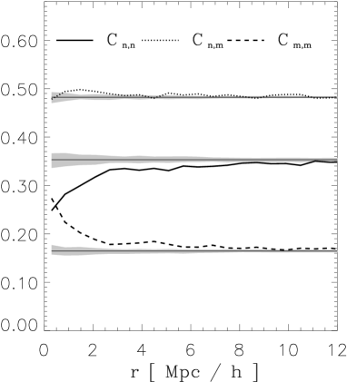
Figure 3: Conditional cross–correlation function of halos with (m) and without (n) major merger in their evolution history. The shaded area is obtained by randomizing the assignment among the halos (see text for details). The subsamples were selected from the total sample of halos with $v_{\rm circ}>100$km/s.

To investigate the significance of these deviations we performed a non–parametric Monte Carlo test (Besag & Diggle, 1977), similar to the one used in Kerscher et al. (2001) and Kerscher (1998). Our null hypothesis is “no mark correlation”. We simulate this null hypotheses by keeping the positions of the halos fixed and randomly re-assigning the marks (in this case the class assignments) to the halos. We repeat this to generate 99 realizations of this null hypothesis. The shaded areas in Fig. 3 are the one–$\sigma$ regions numerically determined from these samples. To quantify the significance we have to define a distance measure. Using $M=4$ equidistant radii $r_{i}$ in the range from 0.8$h^{-1}$Mpc to 2.8$h^{-1}$Mpc we define the “distance” of the $k$–th sample to the expected value for no mark correlation:

$$d^{k}=\frac{1}{M}\sum_{i=1}^{M}\Big{(}C_{m,m}(r_{i})-\frac{\varrho_{m}^{2}}{\varrho^{2}}\Big{)}^{2},$$ (11)

with the overall number density $\varrho$ and the number density $\varrho_{m}$ of merged halos. Similarly we determine the distance $d^{\rm halo}$ of the original halo sample to the null hypothesis. Then we sort all the $d$’s and determine the position of $d^{\rm halo}$. In this case $d^{\rm halo}$ is the fifth largest distance, and we conclude that the original halo sample is incompatible with the null hypothesis ”no mark correlation” at a significance level of 95% (see the comments by Marriott 1978 concerning the significance level).

Figure 4 shows the conditional cross–correlations of the three subsamples which we considered above using the two–point correlation function (Fig. 2: the halos which never underwent a major merger in the past, sample n; early major merger at $z>1$, sample e; and late major merger at $0\leq z\leq 1$, sample l).

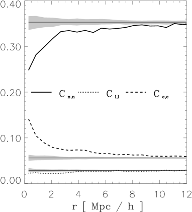
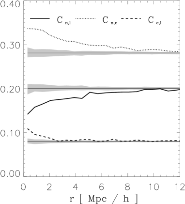
Figure 4: Conditional cross–correlations of halo subsamples defined using the epoch or absence of the last major merger (e: the last major merger at $z>1$, l: at $z<1$, n: never occured). The shaded area is obtained by randomizing the assignment among the halos (see text for details). The subsamples were selected from the total sample of halos with $v_{\rm circ}>100$km/s.

As before, positive $C_{\rm e,e}$ at small separations indicates that for objects at distances less than about 2 $h^{-1}$Mpc the halos with a major merger in their early formation history are relative over–abundant, at the expense of halos without a major merger, as deduced from the lowered $C_{\rm n,n}$. This signal is most prominent on scales below 3$h^{-1}$Mpc but it extends out to 10$h^{-1}$Mpc in agreement with the enhanced two-point correlation function of that subsample (Fig. 2). We interpret this as indication of a high number of early merged halos in clusters. The signal has high significance and it is not influenced by uncertainties in the normalization of the correlation function that may be caused by selection effects. Interestingly, the halos with a late major merger show no excess correlations but rather a lowered abundance on small scales, also manifested as the lower correlation function amplitude of that subsample.

The lower panel of Fig. 4 shows the cross-correlation of halos from different evolution classes. The over-abundance of pairs of never and early merged halos reflects the continuous accretion process onto high density regions. Infalling isolated halos from less dense regions accrete onto higher density regions with high velocity dispersions and, thus, low probability of merging. Therefore, type-n halos can survive in the high-density regions relatively long which explains the increasing of $C_{\rm n,e}$ towards small scales. The opposite is true for never $n$ and late $l$ merged halos. Type-l halos located predominantly in groups where mergers are more likely due to the lower velocity dispersions. The probability of accreting type-n halo (located close to an type-l halo) to experience a merger in high-density regions is therefore high. Many such halos will thus disappear (will become l-halos) resulting in suppression of $C_{\rm n,l}$ amplitude at small separations.

Note, that these features are qualitatively independent from a lower cut in the circular velocity $v_{\rm circ}$, but the amplitude and the spatial range is reduced if we consider more massive halos with $v_{\rm circ}>120$km/s or $v_{\rm circ}>150$km/s. This is due to the higher number of mergers within the low circular velocity halos.

Let us now consider halos which lost a substantial part of their mass due to tidal interactions. Figure 5 shows the conditional cross–correlation function of the halos using two classes: no stripping (sample: ns) and stripped (sample: s). Positive $C_{\rm s,s}$ at $r<5h^{-1}{\rm\ Mpc}$ indicates that the number of stripped pairs is strongly enhanced at these separations, whereas the number of non–stripped pairs is reduced. This result is in accordance with the strongly enhanced correlation function shown in Fig. 2. In fact, we expect to find stripped halos only in the environment of clusters. The results for samples with a higher cut in the circular velocity $v_{\rm circ}>150$km/s are very similar.

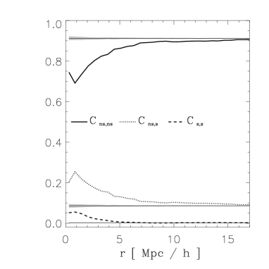
Figure 5: Conditional cross–correlations of halos with (s for stripped) and without (ns) loss of mass in their mass evolution history (selected from the sample of halos with $v_{\rm circ}>100$km/s).

4.3 Spatial distribution and circular velocity

As mentioned in Sec. 2, the mass and the maximum circular velocity of halos are tightly related. At the same time, the circular velocity can be determined more reliably in simulation as well as in observations, either through direct measurement using emission line width or rotation curve or via galaxy luminosity using the Tully-Fisher and the Faber-Jackson relations. Therefore, it is interesting to explore galaxy mark correlations with the maximum circular velocity as mark. This would mimic to some degree luminosity segregation effects in observed galaxy samples. Figure 6 shows the mark correlation functions of halos at $z=0$ with the circular velocity as mark. There is a strong signal in $k_{m}(r)$ at small separations but the signal is significant even out to 10$h^{-1}$Mpc . This indicates that the mean circular velocity of pairs of halos with separations below $\sim 10$$h^{-1}$Mpc is larger than the overall mean circular velocity $\overline{v}_{\rm circ}$ of the parent halo sample.

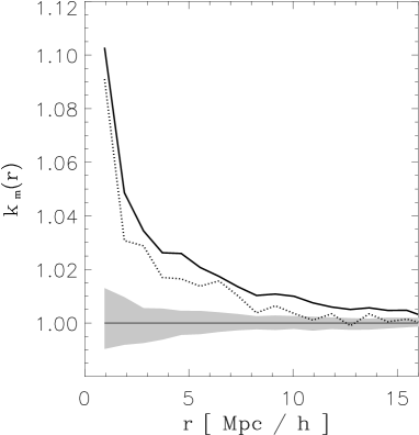
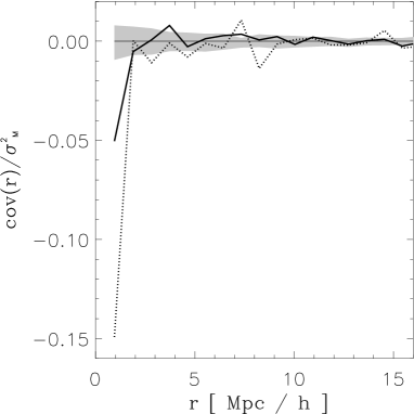
Figure 6: The mark correlation functions $k_{m}(r)$ and ${{\text{{\it cov}}}}(r)$ (see Eqs. 6 and 3.1) for halos with the circular velocity $v_{\rm circ}$ as a scalar mark. Two lower cut-offs have been used: $v_{\rm circ}>100$km/s (solid line) and $v_{\rm circ}>150$km/s (dotted line). The shaded area is obtained by randomizing the mark among the halos.

The negative signal of ${{\text{{\it cov}}}}(r)$ is confined to small separations ($\lesssim 2$$h^{-1}$Mpc). This is because pairs at small separations are more frequently built from one halo with circular velocity larger than $\overline{v}_{\rm circ}$ and the other halo with circular velocity smaller than $\overline{v}_{\rm circ}$. Hence, this signal is dominated by pairs of small-mass subhalos and massive parent halos. The mark correlations results for both samples with $v_{\rm circ}>100$km/s and $v_{\rm circ}>150$km/s are shown. The mean mark correlation function, $k_{m}(r)$, exhibits a slightly stronger signal for the sample with a lower cut in circular velocity, but the signal ${{\text{{\it cov}}}}(r)$ is weaker for $v_{\rm circ}>100$km/s. The latter is due to the considerably larger number of isolated small-mass halos; i.e. in addition to pairs between large- and small-mass halos, for the $v_{\rm circ}>100$km/s sample there are many more small–small mass pairs.

Figure 7 shows the evolution of the conditional covariance ${{\text{{\it cov}}}}(r)$ of the circular velocity with redshift. The conditional covariance is negative at low redshifts out to scales of 2$h^{-1}$Mpc  as discussed above. At high redshifts ($z=2$ and $z=3$), significant positive amplitude of ${{\text{{\it cov}}}}(r)$ indicates that pairs with similar circular velocities are overabundant. At these redshifts the signal is significant out to the scale of $\sim 5$$h^{-1}$Mpc due to the large number of smaller-mass progenitors of the present day halos.

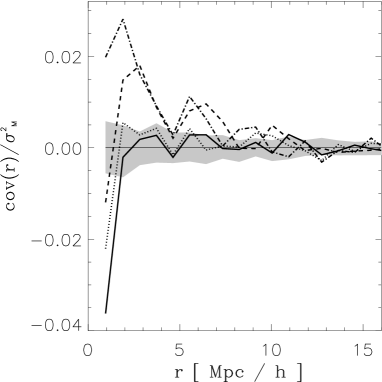
Figure 7: The redshift evolution of the mark correlation function ${{\text{{\it cov}}}}(r)$ for halos with the circular velocity $v_{\rm circ}$ as a scalar mark and a lower cut-off of $v_{\rm circ}>100$km/s: $z=0$ (solid line), $z=1$ (dotted line), $z=2$ (dashed line), $z=3$ (dashed dotted line). The shaded area is obtained by randomizing the mark among the halos.

5 Discussion and conclusions

In the previous section we used a novel statistical tool, the mark correlation functions, to study clustering of galactic halos as a function of their properties and environment in a high-resolution numerical simulation of the $\Lambda$CDM cosmology. We applied MCFs using several types of continuous and discrete marks: maximum circular velocity, $v_{\rm circ}$, of halos (continuous), merger mark indicating whether halos experienced (m) or not (n) a major merger in their evolution history, a stripping mark (s) indicating whether the halo underwent a tidal stripping (i.e., mass loss) during its evolution (discrete marks). The halos which underwent major merger (m) are further classified by the epoch of the merger: late (l; $z<1$) and early (e; $z>1$) mergers. Our main results are as follows.

The two-point correlation amplitude is different for the halo subsamples with different marks. The halos that experienced an early major merger or mass loss (e and s) are clustered considerably more strongly than the overall halo population, while halos with late or no mergers have correlation function amplitude below that of the overall halo sample. This result indicates that halo clustering depends sensitively on the details of their evolution history. If existence of a major merger during halo evolution is related to the morphology of galaxies that halos host, the above result indicates that early type galaxies and galaxies in clusters and groups (hosted by halos that undergo tidal stripping) should be clustered more strongly than the late type galaxies and the overall galaxy population. Qualitatively, such trend exists in the observed galaxy samples (e.g., Hermit et al., 1996; Guzzo et al., 1997; Zehavi, 2002) implying that the morphology-dependent clustering may be largely due to the overall merger history of the galactic halos.

Using maximum circular velocity of halos as a continuous mark, we found that at $z=0$ the mean circular velocity of pairs of halos with separations $\lesssim 10$$h^{-1}$Mpc is larger than the overall mean circular velocity $\overline{v}_{\rm circ}$ of the parent halo sample (manifested as significant enhancement of the mean mark at these separations; see Fig 6). Moreover, the negative mark covariance (Eq. 3.1) at small separations shows an enhanced abundance of pairs with halo circular velocities above and below the average circular velocity. This mean circular velocity enhancement increases steadily during the evolution of halos from $z=3$ to $z=0$. The mark covariance, $cov(r)$, has a more complicated behavior: it is negative at present, disappears at redshift $z\sim 1$ and becomes positive at higher redshifts due to the larger number of low circular velocity halos (the circular velocity function of halos steepens at high redshifts, see Fig. 1). Although the relation is not direct, the maximum circular velocity of halos should correlate well with the maximum circular velocity or velocity dispersion of the galaxies they host. The enhanced mean circular velocity in small-separation pairs should therefore correspond to the luminosity segregation or luminosity-dependent clustering in the observed galaxies. The luminosity dependence of galaxy clustering was recently convincingly detected in both 2dF (Norberg, 2001) and SDSS (Zehavi, 2002) galaxy surveys.

The mark correlation analysis indicate that galaxy-size halos ($v_{\rm circ}>100$km/s) which experienced a major merger in their evolution history are over-abundant in pairs with separations $\lesssim 3$ $h^{-1}$Mpc with respect to the overall halo population, while halos which never experienced a major merger are under-abundant at these separations. We find no significant cross-correlation between these two halos classes. The overabundance of merger halos is due largely to the halos which experienced a major merger relatively early ($z>1$); halos with late ($z<1$) major merger are not over-abundant (this is also manifested in the low amplitude of their two-point correlation function relative to that of the overall halo population; see Figs. 2, 4). This result can be interpreted as correlation between the time since the last major merger and present-day environment of the halo (i.e., halos which underwent an early major merger tend to be located in clusters and groups). The significance of the results was estimated by a non–parametric Monte Carlo test which showed that the segregation and anti-segregation have significance of $>95$% in the distance range 0.8$h^{-1}$Mpc to 2.8$h^{-1}$Mpc . Similarly, the probability of finding stripped halos in pairs of separations $\lesssim 5$$h^{-1}$Mpc is twice higher than the corresponding probability for the overall halo sample. Halos which experienced early major mergers and/or mass loss due to tidal stripping are likely to host early type galaxies. In this case, the above mark correlation results for DM halos indicate that morphological segregation of galaxies may be due to the specifics of the mass evolution histories and environment of their parent halos.

The analysis presented in this paper showed that MCFs provide powerful, yet algorithmically simple, quantitative measures of segregation in halo spatial distribution with respect to their properties (e.g., maximum circular velocity) and merger history (e.g., time since the last major merger). The mark correlation functions allow us to quantify the degree of segregation as a function of scale and can be used to quantify the differences in the spatial distributions of various galaxy samples (similarly to the usual two-point correlation function) and, at the same time, to study the interplay between the spatial clustering and the distribution of galaxy properties (marks). In this respect, the MCFs are a natural extension of the spatial correlation functions for studies where it is advantageous to consider mark and spatial distributions simultaneously. We believe that this will make the mark correlation functions very useful for analysis of spatial clustering and segregation as a function of various galaxy properties in current (SDSS and 2dF) and future (e.g., DEEP2) large redshift surveys.