Line formation in convective stellar atmospheres

In an effort to estimate the largely unknown effects of photospheric temperature fluctuations on spectroscopic abundance determinations, we have studied the problem of LTE line formation in the inhomogeneous solar photosphere based on detailed 2-dimensional radiation hydrodynamics simulations of the convective surface layers of the Sun. By means of a strictly differential 1D/2D comparison of the emergent equivalent widths, we have derived “granulation abundance corrections” for individual lines, which have to be applied to standard abundance determinations based on homogeneous 1D model atmospheres in order to correct for the influence of the photospheric temperature fluctuations. In general, we find a line strengthening in the presence of temperature inhomogeneities as a consequence of the non-linear temperature dependence of the line opacity. The resulting corrections are negligible for lines with an excitation potential around $E_{i}=5$ eV, regardless of element and ionization stage. Moderate granulation effects ($\Delta_{\rm gran}\approx-0.1$ dex) are obtained for weak, high-excitation lines ($E_{i}\ga 10$ eV) of C i, N i, O i as well as Mg ii and Si ii. The largest corrections are found for ground state lines ($E_{i}=0$ eV) of neutral atoms with an ionization potential between 6 and 8 eV like Mg i, Ca i, Ti i, Fe i, amounting to $\Delta_{\rm gran}\approx-0.3$ dex in the case of Ti i. For many lines of practical relevance, the magnitude of the abundance correction may be estimated from interpolation in the tables and graphs provided with this paper. The application of abundance corrections may often be an acceptable alternative to a detailed fitting of individual line profiles based on hydrodynamical simulations. The present study should be helpful in providing upper bounds for possible errors of spectroscopic abundance analyses, and for identifying spectral lines which are least sensitive to the influence of photospheric temperature inhomogeneities.

1 Introduction

Theoretical model atmospheres serve as the fundamental tool for the quantitative analysis of stellar spectra. The basic parameters of a stellar atmosphere – effective temperature, surface gravity, and chemical composition – can be inferred from the comparison between observed and calculated spectra. Much effort has been spent to improve the theoretical models by incorporating as much realistic physics as possible. Specifically, in late-type stars one is confronted with the problem of a detailed treatment of both radiative and convective energy transport. A high degree of sophistication has been achieved in modeling radiative transfer: standard stellar atmosphere codes can now handle the influence of millions of spectral lines.

In contrast, the treatment of convection is still rather crude. Usually, stellar atmospheres are described as 1-dimensional hydrostatic configurations where the convective energy transport is calculated from the so-called mixing-length theory (MLT, Vitense V53 (1953); Böhm-Vitense BV58 (1958)) or variants thereof (e.g. Canuto et al.CGM96 (1996)). However, modern spectroscopic observations have reached a level of precision that requires improved model atmospheres for a reliable interpretation, including a proper treatment of hydrodynamical phenomena.

From the point of view of standard model atmospheres, convection affects the temperature structure in a twofold way: it influences the mean vertical stratification and introduces horizontal inhomogeneities. MLT is designed to model only the mean structure and is not suitable to construct realistic multi-component model atmospheres. Although realistic hydrodynamical model atmospheres do exist for the Sun and a few solar-type stars due to the pioneering work by Nordlund (No82 (1982)), Nordlund & Dravins (ND90 (1990)), Stein & Nordlund (SN89 (1989), SN98 (1998)), and Ludwig et al. (LFS99 (1999)), to name just a few important contributions, such complex models are not usually applied for the analysis of stellar spectra.

Observationally, the solar granulation is the visible imprint of thermal convection extending far into the photospheric layers where spectral lines are formed. The effect of the associated photospheric temperature inhomogeneities on the line formation process and the consequences for spectroscopic abundance determinations are not yet well understood, but it is generally believed that the errors introduced by representing a dynamic, inhomogeneous atmosphere by a static, plane-parallel model are small. However, reliable quantitative estimates of this effect are difficult to find. Earlier studies suffer from uncertainties in the underlying empirical two-component models, which are rather ad hoc and lack a firm physical foundation (e.g. Hermsen He82 (1982)). Later investigations based on relatively crude numerical convection models (Atroshchenko & Gadun AG94 (1994); Gadun & Pavlenko GP97 (1997)) led to questionable and partly ambiguous conclusions. Recent determinations of the solar photospheric Fe and Si abundance by Asplund et al. (2000b ) and Asplund (2000a ), respectively, rely on state-of-the-art 3D numerical convection simulations and take all hydrodynamical effects fully into account. However, comparison of these results with those based on the empirical 1D Holweger-Müller (HM74 (1974)) solar atmosphere does not allow to separate the influence of inhomogeneities from the effect of the mean stratification, and to study the 1D/3D abundance corrections as a function of the line parameters in a systematic way.

In this work we investigate the spectroscopic effects of horizontal temperature inhomogeneities in the solar atmosphere based on detailed 2D hydrodynamical models of solar surface convection (Freytag et al. FLS96 (1996); Ludwig et al. LFS99 (1999), Steffen S00 (2000)). We do not address the question whether the mean temperature structure supplied by MLT is an appropriate representation of the mean stratification obtained from hydrodynamical simulations (the problem of the ‘right’ choice of the mixing-length parameter $\alpha$ for recovering the correct mean temperature stratification was investigated by Steffen et al. (SLF95 (1995)) in the context of white dwarf atmospheres). Rather, our main question is: how large are the systematic errors of standard spectroscopic abundance determinations due to the fact that one replaces the ‘real’ line profile, which actually is the result of averaging the spatially resolved line intensities over the granulation pattern, by the line profile computed from a single plane-parallel temperature stratification?

In Sect. 2, we introduce a simple analytical argument to illustrate the basic effect of line strengthening in the presence of temperature fluctuations. Then we summarize the main characteristics of the numerical simulations of solar surface convection in Sect. 3, outline our method to derive ‘granulation abundance corrections’ from a differential 1D/2D comparison of computed line equivalent widths in Sect. 4, before finally presenting the results for the Sun in Sect. 5. A summary of our findings is given in Sect. 6.

In order to give a physical explanation for the numerical results obtained in this work, we have carried out a detailed investigation the process of LTE line formation in an inhomogeneous stellar atmosphere based on the analysis of the transfer equation and the evaluation of line depression contribution functions. This study is presented in the second paper of this series (Paper II).

2 A simple analytical illustration

The strength of a spectral line formed in a plane-parallel (1D) atmosphere will differ from the strength of the same line formed in an inhomogeneous atmosphere with the same chemical composition and mean temperature stratification because, in general, there is a non-linear relationship between line strength and temperature. It may be expected that lines with a very high excitation potential are most affected because (i) they originate from deep layers where convection is well developed, and (ii) they are highly sensitive to temperature fluctuations. Likewise, the molecular equilibrium is known to be highly sensitive to temperature fluctuations, so molecular lines might also be strongly affected if the temperature inhomogeneities reach the higher photosphere where these lines are formed.

Figure 1: Spatial variation of $W$ for a sinusoidal temperature variation according to Eq.(6), for $\sigma=0.05$ and $E_{i}=10$ eV. Averaging over one spatial wavelength gives $\langle W\rangle/W_{0}=1.78$ (dotted horizontal line).

As an illustration of the expected effect, consider the following simple analytical argument. Assume that the equivalent width of a weak line $W$ depends exponentially on the inverse temperature $\theta=5040/T$, as suggested by the form of the Saha-Boltzmann equations,

$$W(\Delta\theta)=W_{0}\exp\left\{-E_{i}\Delta\theta\ln 10\right\},$$ (1)

where $E_{i}$ is the excitation potential in eV and $\Delta\theta=\theta-\theta_{0}$. Assume further that $\theta$ is normally distributed about the mean $\theta_{0}$ with standard deviation $\sigma$,

$$g(\Delta\theta)=\frac{1}{\sigma\sqrt{2\pi}}\exp\left\{-\frac{\Delta\theta^{2}}{2\sigma^{2}}\right\}.$$ (2)

Then it can be shown by analytical integration that

$$\langle W\rangle = \int_{-\infty}^{+\infty}g(\Delta\theta)\,W(\Delta\theta)\,\mathrm{d}\Delta\theta$$ (3)

$$= W_{0}\exp\left\{\frac{1}{2}E_{i}^{2}\sigma^{2}(\ln 10)^{2}\right\}$$

i.e. the mean value $\langle W\rangle$ of the equivalent width formed in an inhomogeneous medium is always greater than the equivalent width for the unperturbed medium, $W_{0}$. As long as $E_{i}\sigma$ is small enough, the effect is negligible, but this is not true in general. Assuming $\sigma=0.05$, corresponding to 6% temperature fluctuation around $T_{0}$ = 6000 K, and $E_{i}=10$ eV, the effect is very substantial: $\langle W\rangle\approx 2\,W_{0}$, i.e. the elemental abundance derived from such lines would be overestimated by a factor of 2! Note that, for example, several important neutral oxygen lines have $E_{i}$ between 9 and 11 eV.

A similar result is obtained when assuming a totally different distribution of $\Delta\theta$,

$$f(\Delta\theta)=\frac{1}{\pi\sqrt{2\sigma^{2}-\Delta\theta^{2}}},$$ (4)

corresponding to sinusoidal temperature fluctuations in one horizontal direction,

$$\Delta\theta=\sigma\sqrt{2}\sin(2\pi x),$$ (5)

where $x$ is the spatial coordinate. According to Eq.(1), the fluctuation of the equivalent width is then

$$W(x)=W_{0}\exp\left\{-E_{i}\ln 10\,\sigma\sqrt{2}\sin(2\pi x)\right\}.$$ (6)

Adopting again $\sigma=0.05$ and $E_{i}=10$ eV, we have plotted $W(x)$ in Fig. 1. Clearly, the fluctuation of $W$ is highly asymmetric with respect to $W_{0}$, and numerical averaging over one spatial wavelength gives $\langle W\rangle\approx 1.8\,W_{0}$.

Looking at Table 1, it turns out that the simple model severely overestimates the abundance correction in the case of the oxygen lines mentioned as an example above. This is because, in reality, the line formation process is much more complicated, since the line strength depends not only on the line opacity but also on the continuum opacity and on the local temperature gradient of the atmosphere (see Paper II). Moreover, spectral lines usually form over a substantial depth range, and the sign of $\Delta\theta$ may depend on depth, leading to partial cancellation of the local effects, especially for stronger lines. Finally, saturation can play a significant role as well. Hence, realistic abundance corrections can only be derived from detailed line formation calculations based on multi-dimensional hydrodynamical model atmospheres.

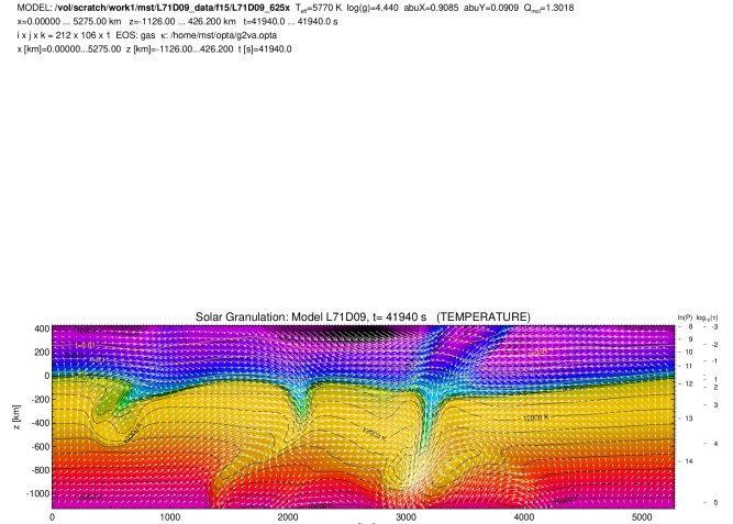
Figure 2: Snapshot from a 2-dimensional numerical simulation of solar surface convection after 41 940 s of simulated time. This model was computed on a Cartesian grid with 210x106 mesh points (tick marks along upper and right side), with periodic lateral boundary conditions ($L=5\,250$ km). “Open” boundary conditions at the bottom and top of the computational domain are designed to minimize artificial distortions of the flow. The velocity field is represented by pseudo streamlines, indicating the displacement of a test particle over 20 sec (maximum velocity is 10.1 km/s at this moment); the temperature structure is outlined by temperature contours in steps of 500 K. Geometrical height $z=0$ (scale at left) corresponds to $\tau_{\rm Ross}\approx 1$; scales at right refer to the horizontally averaged gas pressure [dyn cm^-2] and Rosseland optical depth $\tau_{\rm Ross}$.

3 Time-dependent Radiation Hydrodynamics

In order to adequately address the complex problem outlined above, we have investigated the effects of temperature inhomogeneities on the formation of a variety of spectral lines by means of a realistic 2-D radiation hydrodynamics (RHD) simulation of solar surface convection. In the following, we briefly summarize the foundations of the hydrodynamical simulation and the main results concerning the solar photosphere.

3.1 2-dimensional numerical simulation

Stellar surface convection is governed by the conservation equations of hydrodynamics, coupled with the equations of radiative energy transfer. Our hydrodynamical models result from the numerical integration of this set of partial differential equations. This approach constitutes an increasingly powerful tool to study in detail the time-dependent hydrodynamical properties of the solar granulation.

Just like ‘classical’ stellar atmospheres, the hydrodynamical models are characterized by effective temperature, $T_{\rm eff}$, surface gravity, $g$, and chemical composition of the stellar matter. But in contrast to the mixing-length models, they account for ‘overshoot’ and no longer have any free parameter to adjust the efficiency of the convective energy transport. Based on first principles, RHD simulations provide physically consistent ab initio models of stellar convection which can serve to address a variety of questions, including the problem of line formation in inhomogeneous stellar atmospheres.

The models used for the present investigation comprise a small section near the solar surface, extending over 7 pressure scale heights in the vertical direction, including the photosphere, the thermal boundary layer near optical depth $\tau_{\rm Ross}=1$, and parts of the subphotospheric layers. Only the uppermost layers of the deep solar convection zone can be included in the model, requiring an open lower boundary. The simulations are designed to resolve the solar granulation. The effect of the smaller scales, which cannot be resolved numerically, is modeled by means of a subgrid scale viscosity (so-called Large Eddy Simulation approach). Spatial scales larger than the computational box are unaccounted for. We employ a realistic equation of state, including ionization of H, HeI, HeII and H₂ molecule formation. In order to avoid problematic simplifications like the diffusion or Eddington approximation, we solve the non-local radiative transfer problem along a large number ($N_{\rm x}\,f_{\rm sub}\,N_{\theta}\,N_{\phi}=210\cdot 4\cdot 2\cdot 8\approx 10\,000$) of rays in 5 opacity bins, with realistic opacities accounting adequately for the influence of spectral lines (see Nordlund No82 (1982), Ludwig Lu92 (1992)). For further details see Ludwig et al. (LJS94 (1994)), Freytag et al. (FLS96 (1996)), Ludwig et al. (LFS99 (1999)), Steffen (S00 (2000)).

3.2 Main results

The basic features of the numerical convection model are illustrated in Fig. 2, showing a representative snapshot from a well-relaxed simulation of the solar granulation. In the convectively unstable, subphotospheric layers, fast ($v\la c_{s})$ narrow downdrafts (also called plumes or jets) stand out as the most prominent feature. They are embedded in broad ascending regions (the granules) where velocities are significantly lower. We find enormous temperature differences between the cool downflows and the hot upflows ($\Delta T_{\rm max}\approx 5\,000$ K at $z\approx-100$ km). Near optical depth $\tau=1$, efficient radiative surface cooling produces a very thin thermal boundary layer over the ascending parts of the flow, where the temperature drops sharply with height ($\Delta T/\Delta z\approx 80$ K/km, see upper panel of Fig. 3) and the gas density exhibits a local inversion. Note however, that the temperature contrast is much reduced on the optical depth scale (see bottom panel of Fig. 3).

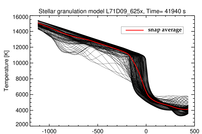
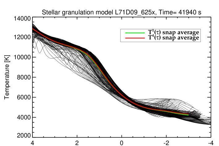
Figure 3: Temperature as a function of geometrical depth $z$ (top) and as a function of individual optical depth $\tau_{\rm Ross}$ (bottom) for the snapshot shown in Fig. 2. Each line corresponds to a different $x$ position. Note that the $\langle T\rangle$ and the $\langle T^{4}\rangle^{1/4}$ average are hardly distinguishable in this representation.

Although convectively stable according to the Schwarzschild criterion, the photosphere ($\tau\la 1$) is by no means static. Convective flows overshooting into the stable layers from below are decelerated here and deflected sideways. This can sometimes result in transonic horizontal streams which lead to the formation of shocks in the vicinity of strong downdrafts (see vertical fronts in Fig. 2 between $3\,000<x<3\,500$ km, $z\ga 100$ km).

Oscillations excited by the stochastic convective motions contribute to the photospheric velocity field as well. Interestingly, the oscillation periods lie in the range 150 to 500 s for the solar simulation, in close agreement with the observed 5 minute oscillations. Controlled by the balance between dynamical cooling due to adiabatic expansion and radiative heating in the spectral lines, the mean photospheric temperature stratification is slightly cooler than in radiative equilibrium, and the resulting temperature structure is not at all plane-parallel.

According to Eq.(3), the line strengthening depends on the key quantity $\sigma=\theta_{0}\,\delta T_{\rm rms}/T_{0}$, where $\delta T_{\rm rms}=\sqrt{\langle(T-T_{0})^{2}\rangle}$. We have evaluated $\delta T_{\rm rms}$ as a function of optical depth for our 2D numerical simulation of solar convection (Fig. 4). For the problem under investigation, temperature differences have to be taken over levels of constant optical depth, rather than at constant geometrical depth. According to the simulations, typical values in the lower photosphere are in the range $0.04<\delta T_{\rm rms}<0.06$. The minimum near $\log\tau_{\rm Ross}=-0.5$ is related to the ‘inversion’ of the temperature fluctuations at this height.

It is worth mentioning that we have recently carried out fully 3-dimensional simulations with a new code developed by B. Freytag and M. Steffen (Freytag; Steffen et al., in preparation). We find that the depth dependence of $\delta T_{\rm rms}(\tau)$ is qualitatively similar in 2D and 3D. However, the amplitude of the temperature fluctuations is systematically smaller at all heights in the 3D simulation. The difference is most pronounced in the higher photosphere (see Fig. 4).

3.3 Accuracy of 2D and 3D convection models

The straightforward application of hydrodynamics and radiative transfer simulations is certainly the most satisfactory and consistent method to treat the line formation in a convective stellar atmosphere, although the outcome is difficult to check by independent analysis. The hydrodynamical models presented here must be regarded as somewhat preliminary for several reasons. First of all, the restriction of the flow geometry to 2 dimensions must lead to deviations from the true 3D atmospheric structure. As a consequence, the convective line shift and asymmetry predicted by the 2D granulation models is quantitatively different from that obtained with 3D models (Asplund et al. 2000a ). A further problem is the relatively poor spatial resolution of the simulations (especially in the vertical direction), which is barely sufficient to resolve the thin thermal boundary layer near $\tau=1$. Certainly, the Reynolds number of the simulations is many orders of magnitude below realistic values. Finally, the influence of the spectral lines on the radiative energy balance can be treated only in an approximate way. Typically, a few opacity bins are used in the simulations, as compared to thousands of frequency points in standard 1D models.

The latter problems apply to state-of-the-art 3D convection simulations as well. We note that a perfect line profile fitting does not necessarily imply a perfect model atmosphere. Another important diagnostic is the center-to-limb variation of the continuum intensity. Even the best 3D solar granulation models still fail to reproduce the observed continuum properties with high accuracy (Asplund et al. ANT99 (1999)), indicating that “the temperature structure close to the continuum forming layers could be somewhat too steep”.

In view of the above mentioned limitations, we prefer to avoid a direct application of our convection simulations. Instead, we favor the somewhat less powerful but more reliable differential approach described in the following section.

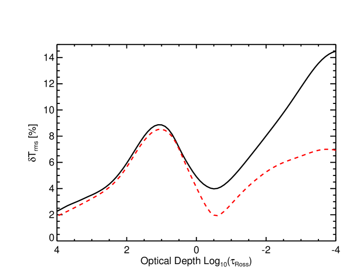
Figure 4: Time-averaged amplitude of rms temperature fluctuations as a function of Rosseland optical depth, derived from the numerical simulation of solar granulation described in Sect. 3 (solid). $\delta T_{\rm rms}$ was obtained by averaging over surfaces of constant Rosseland optical depth for each snapshot and subsequently taking a long-term time average. For comparison, we show corresponding results from a 3-dimensional numerical simulations (dashed) recently carried out with a new code by B. Freytag and M. Steffen.

4 Granulation abundance corrections

4.1 The problem

The problem we want to address is the following. Assume you have the ‘best possible’ 1D representation of the solar atmosphere, correctly reproducing the continuum intensity distribution $I_{\lambda}(\lambda)$ and its center-to-limb variation $I_{\lambda}(\mu)$. The microturbulence parameter $\xi_{\rm mic}$ is adjusted such as to minimize the overall dependence of the derived abundances on line strength. The empirical Holweger-Müller (HM74 (1974)) atmosphere comes close to this ideal mean temperature structure. In the presence of temperature fluctuations, however, non-linearities in the line formation process will inevitably lead to systematic errors of abundance determinations based on individual spectral lines. The present work aims at quantifying this kind of error.

We have adopted a strictly differential procedure to quantify these errors. The basic idea is to identify our 2D hydrodynamical convection simulations with the real inhomogeneous atmosphere, and the mean structure of the simulations with the ‘best possible’ 1D representation. Note that it is not important for the hydrodynamical convection models to reproduce the mean temperature structure of the real solar atmosphere with great precision, because the related errors cancel to a first approximation in our differential comparison. Similarly, the details of the hydrodynamical velocity field are of secondary importance in the present context, since such 1D/2D differences are largely eliminated by a proper choice of the microturbulence parameter. In contrast, there is no free parameter to account for the presence photospheric temperature inhomogeneities. This is why we focus on the abundance corrections related to temperature fluctuations $\delta T_{\rm rms}$ only. The most important quantity to be provided by the convection model is therefore the magnitude and height dependence of $\delta T_{\rm rms}$.

In the following, we outline our method to derive LTE “granulation abundance corrections”, $\Delta_{\rm gran}$, which must be added to the logarithmic elemental abundance derived from standard 1D model atmosphere analysis in order to compensate for the effects of temperature inhomogeneities. Note that our procedure ensures that the corrections $\Delta_{\rm gran}\rightarrow 0$ for vanishing horizontal temperature and pressure fluctuations.

4.2 The procedure

First we have selected $S=11$ representative snapshots from our time-dependent convection simulation (see Sect. 3). These snapshots (one of them shown in Figs. 2 and 3) all have the correct effective temperature (the horizontally averaged radiative energy flux lies within $\pm 1\%$ of the nominal solar flux), but differ in the number and size distribution of granules and in the continuum intensity contrast ($\delta I_{\rm rms}$ varies between 18.0 and 26.5% at $\lambda\,5000$ Å). For each of the 2D snapshots ($s=1\,..\,11$) we then constructed a corresponding 1D model by averaging temperature $T$ and gas pressure $P$ over the corrugated surfaces of constant Rosseland optical depth:

$$T_{\rm s,1D}(\tau_{\rm Ross})=\left\langle T^{4}_{\rm s,2D}(\tau_{\rm Ross},x)\right\rangle^{1/4},$$ (7)

$$P_{\rm s,1D}(\tau_{\rm Ross})=\left\langle P_{\rm s,2D}(\tau_{\rm Ross},x)\right\rangle,$$ (8)

where $\langle.\rangle$ denotes averaging over the horizontal coordinate $x$. Note that the 1D models constructed in this way have very nearly the same radiative flux as the underlying 2D models.

Next we compute, for given elemental abundance and atomic line parameters, the equivalent width of any given spectral line from (i) the set of 2D snapshots by horizontal averaging of the spatially resolved synthetic line profile

$$W_{\rm s,2D}=\left\langle I_{\rm c,s}(x)\,W_{\rm s,2D}(x)\right\rangle/\left\langle I_{\rm c,s}(x)\right\rangle,$$ (9)

where $I_{\rm c}(x)$ is the local continuum intensity, and (ii) from the corresponding 1D models, resulting in $W_{\rm s,1D}$.

For the line formation calculations, we employed the Kiel spectrum synthesis code LINFOR under the assumption of LTE. For the 1D atmospheres, we have always adopted a depth-independent microturbulence velocity of $\xi_{\rm mic}=1$ km/s. For snapshots from the convection simulations we have computed synthetic spectra for two different assumptions concerning the non-thermal velocity field: in case (A) we used the depth-dependent hydrodynamical velocity field $v(x,z)$ obtained from the simulations, in case (B) we replaced the hydrodynamical velocity field by a depth-independent microturbulence velocity $\xi_{\rm mic}=1$ km/s.

As the final step, we calculate the mean equivalent widths resulting from the set of 1D and 2D line profiles, $W_{\rm 1D}=\frac{1}{S}\,\sum_{s=1}^{S}W_{\rm s,1D}$ and $W_{\rm 2D}=\frac{1}{S}\,\sum_{s=1}^{S}W_{\rm s,2D}$, respectively. For truly weak lines, the (logarithmic) “granulation abundance correction” would simply be

$$\Delta_{\rm gran}^{\rm weak\;lines}=\log W_{\rm 1D}-\log W{\rm 2D}.$$ (10)

In general, however, the equivalent width is not proportional to the elemental abundance due to saturation. We account for these curve-of-growth effects in the following way. Knowing that the ‘true’ abundance, $N_{\rm 2D}$ produces the equivalent width $W_{\rm 2D}$ with the 2D inhomogeneous model atmosphere (and $W_{\rm 1D}$ with the 1D mean structure), we iteratively determine the elemental abundance $N_{\rm 1D}$ which produces the equivalent width $W_{\rm 2D}$ with the 1D mean stratification. The “granulation abundance correction” is then given by

$$\Delta_{\rm gran}=\log N_{\rm 2D}-\log N_{\rm 1D}.$$ (11)

For simplicity, we used the standard HM model atmosphere (Holweger & Müller HM74 (1974); $\xi_{\rm mic}=1$ km/s) for this final step of the procedure ($W_{\rm 1D}\rightarrow N_{\rm 2D}$, $W_{\rm 2D}\rightarrow N_{\rm 1D}$). This is justified because all we need is a realistic curve-of-growth, $W(N)$, which is very similar for the averaged simulation snapshots and the HM atmosphere.

Case (A) and (B) give essentially the same corrections for weak lines, but the results may differ substantially for stronger lines, where $W_{\rm 2D,A}<W_{\rm 2D,B}$ (implying that the hydrodynamical velocity field provides an effective ‘microturbulence’ $\xi_{\rm mic}({\rm RHD})<1$ km/s). For lines of arbitrary strength, we strongly favor the granulation corrections derived from case (B), because this strictly differential 1D/2D comparison is based on the same non-thermal velocity field, and thus cleanly separates the effect of the temperature inhomogeneities from that of the small-scale velocity field. In the following, $\Delta_{\rm gran}$ therefore denotes the granulation abundance corrections derived from case (B).

For practical reasons, we have used only a small number of snapshots ($S=11$) for our present investigation. The statistical uncertainty of the derived abundance corrections is therefore appreciable. In order to quantify this uncertainty, we have also tabulated the standard deviation of the corrections $\Delta_{\rm gran}$,

$$\sigma=\sqrt{\frac{1}{S-1}\sum_{s=1}^{S}\left(\Delta_{\rm gran,s}-\overline{\Delta_{\rm gran}}\right)^{2}},$$ (12)

derived from the 11 individual snapshots. The quantity $\sigma$ can serve to judge the significance of the abundance corrections for each of the lines listed in the tables below.

5 Results for the Sun

We have applied the above procedure to a representative sample of lines, covering different elements, ionization stages, ionization energies, excitation energies, line strengths and wavelengths. In this differential study, we have adopted the same representative van der Waals broadening constant for all lines, $\log C_{6}=-30.3867$ (definition according to Mihalas (Mi78 (1978)), which differs from that by Unsöld (U55 (1955)) by a factor $2\pi$), and have neglected line broadening due to electron collisions, $C_{4}=0$. The results are listed in Tables 1, 2, 3, and 4. Most of the lines are ’fictitious’ lines (‘even’ wavelength entries in the tables), allowing a systematic study of the granulation effect as a function of the line parameters. The tables also contain a number of ’real’ lines (table entries with ‘uneven’ wavelength) for Li, O, and Si, which have already been used with detailed abundance studies by Wedemeyer (SW01 (2001)) and Holweger (HH01 (2001)). In the latter work, the granulation abundance corrections were obtained by interpolation in the list of fictitious lines (Tables 1,3), which covers a sufficient range of the relevant line parameters.

5.1 Atoms with high ionization potential and ions

Atoms with high ionization potential like C i, N i, and O i, as well as singly ionized elements are representative of species in the main ionization stage. Neutral nitrogen (ionization potential $\chi=14.5$ eV) can be taken as the prototype of these species. Unlike C and O, N is not significantly affected by molecule formation or changes in the degree of ionization.

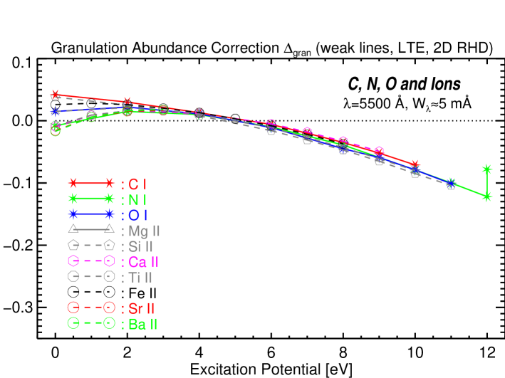
Figure 5: Logarithmic granulation abundance corrections $\Delta_{\rm gran}$ as a function of excitation energy $E_{i}$ for C i, N i, O i, and a number of singly ionized elements, representative of species in the main ionization stage. The plot is based on a subset of weak fictitious lines with $\lambda=5\,500$ Å, $W_{\lambda}\approx 5$ mÅ, taken from Tables 1, 2, 3, 4. The upper symbol at $E_{i}=12$ eV for N i refers to $\lambda\,10\,000$ Å.

Figure 6: Granulation abundance corrections, $\Delta_{\rm gran}$, for the first 8 fictitious nitrogen lines listed in Table 1, compared with test results obtained by increasing the line strength by factors of 5 and 15, respectively.

Figure 7: Granulation abundance corrections, $\Delta_{\rm gran}$, for the first 8 fictitious nitrogen lines listed in Table 1, compared with test results obtained by moving the weak lines from $\lambda=5\,500$ Å to different spectral regions, centered at $\lambda=4\,000$, $8\,000$, $10\,000$, $12\,000$, and $16\,000$ Å, respectively, keeping the reduced equivalent width $W/\lambda$ fixed ($W_{\rm 1D}\approx\lambda/5\,500\cdot 5$ mÅ).

The corrections $\Delta_{\rm gran}$ as a function of excitation energy, $E_{i}$, are displayed in Fig. 5 for our tabulated sample of weak fictitious lines ($\lambda\,5500$ Å, $W\approx 5$ mÅ) of these species. Obviously, the corrections for high-excitation lines of the ‘majority species’ are similar for all elements, and can amount to -0.1 dex for weak lines with $E_{i}\ga 10$ eV. This conclusion is independent of the assumed velocity field which is irrelevant here: $\Delta_{\rm gran,A}\approx\Delta_{\rm gran,B}$ for lines as weak as 5 mÅ (see tables).

5.1.1 Dependence on line strength

The dependence of the granulation abundance corrections on line strength was investigated by test calculations for two additional sets of stronger N i lines. The two set of lines were obtained from the set of N i lines ($\lambda\,5\,500$ Å) listed in Table 1 by increasing their equivalent widths, $W_{\rm 1D}$, by a factor of 5 and 15, respectively. Thus, the test lines in first set of have $W_{\rm 1D}\approx 25$ mÅ, those in the second set $W_{\rm 1D}\approx 80$ mÅ. According to the results shown in Fig. 6, the granulation abundance corrections $\Delta_{\rm gran}$ are systematically more positive for the stronger, otherwise identical lines. For $E_{i}=12$ eV the difference in $\Delta_{\rm gran}$ between the lines with $W_{\rm 1D}\approx 80$ mÅ and $5$ mÅ amounts to +0.07 dex.

5.1.2 Dependence on wavelength

In order to get an idea about the dependence of the granulation abundance corrections on the wavelength of the spectral lines, we also performed test calculations for five additional sets of N i lines, obtained by shifting the weak N i lines listed in Table 1 from $\lambda=5\,500$ Å to $\lambda=4\,000$, $8\,000$, $10\,000$, $12\,000$, and $16\,000$ Å, respectively, enforcing the same reduced equivalent width, $W/\lambda$, i.e. $W_{\rm 1D}\approx\lambda/5\,500\cdot 5$ mÅ.

The results shown in Fig. 7 indicate that the granulation abundance corrections $\Delta_{\rm gran}$ indeed depend on wavelength, in the sense that lines in the blue part of the spectrum show systematically more negative corrections than those in the red part. This general trend is evident over the whole wavelength range, apart from a slight reversal between $\lambda\,8\,000$ and $10\,000$ Å which is related to the Paschen jump at $\lambda\,8208$ Å. For $E_{i}=12$ eV the difference in $\Delta_{\rm gran}$ between a weak line at $\lambda\,4\,000$ and $10\,000$ Å amounts to -0.1 dex.

5.2 Atoms with low ionization potential

Elements with low ionization potential are predominantly singly ionized in the solar atmosphere. The particle density of the remaining neutral atoms of such elements is particularly sensitive to temperature variations. Molecules fall into the same category. Neutral iron (ionization potential $\chi=7.9$ eV) can be taken as representative for these species. According to our models, the fraction of neutral iron is nowhere exceeding 26%; it shows a maximum near $\log\tau_{5500}=-3$ and has dropped to less than 3.5% at $\log\tau_{5500}=0$.

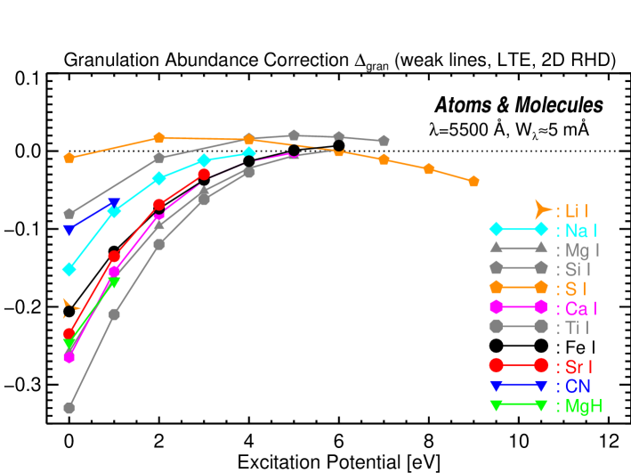
Figure 8: Logarithmic granulation abundance corrections $\Delta_{\rm gran}$ as a function of excitation energy $E_{i}$ for neutral atoms of predominantly ionized elements, and for molecules CN and MgH. The plot is based on a subset of weak fictitious lines with $\lambda=5\,500$ Å, $W_{\lambda}\approx 5$ mÅ, taken from Tables 1, 2, 3, 4.

Figure 9: Granulation abundance corrections, $\Delta_{\rm gran}$, for the 7 fictitious neutral iron lines listed in Table 3, compared with test results obtained by increasing the line strength by factors of 5 and 10, respectively.

Figure 10: Granulation abundance corrections, $\Delta_{\rm gran}$, for the 7 fictitious neutral iron lines listed in Table 3, compared with test results obtained by moving the weak lines from $\lambda=5\,500$ Å to different spectral regions, centered at $\lambda=4\,000$, $8\,000$, $10\,000$, $12\,000$, and $16\,000$ Å, respectively, keeping the reduced equivalent width $W/\lambda$ fixed ($W_{\rm 1D}\approx\lambda/5\,500\cdot 5$ mÅ).

The corrections $\Delta_{\rm gran}$ for a sample of weak fictitious lines ($\lambda\,5500$ Å, $W\approx 5$ mÅ) of these ‘minority species’ are displayed in Fig. 8 as a function of excitation energy, $E_{i}$. We note that the largest granulation effects are found for low-excitation lines of neutral atoms with an ionization potential between 6 and 8 eV. The magnitude of the correction depends on the element and is as large as -0.3 dex for Ti i, $E_{i}=0$ eV. Again, we point out that this result does not depend on the assumed non-thermal velocity field.

It is interesting to note that Asplund (2000a ), using 3D models, finds corrections in the opposite direction for the ’real’ Si I lines listed in Table 2. We emphasize that this is not an indication of fundamentally different “granulation corrections” in 2D and 3D. The corrections given by Asplund with respect to the Holweger-Müller (HM74 (1974)) model include not only the effect of temperature inhomogeneities but also the influence of the different mean stratifications. Obviously, the difference in the mean structure is the more important of the two opposing effects in this case. Indeed, we find from our own models a total correction of -0.05 dex with respect to the Holweger-Müller model, compared to a the tabulated ”granulation correction” of +0.02 dex, explaining the apparently inconsistent results.

5.2.1 Dependence on line strength

As for N i, the dependence of the granulation abundance corrections on line strength was investigated by test calculations for two additional sets of stronger Fe i lines, obtained from the set of Fe i lines listed in Table 3 by increasing their equivalent widths, $W_{\rm 1D}$, by a factor of 5 and 10, respectively. The test lines in first set of have then $W_{\rm 1D}\approx 35$ mÅ, those in the second set $W_{\rm 1D}\approx 70$ mÅ. The results are shown in Fig. 9. Qualitatively, the granulation abundance corrections $\Delta_{\rm gran}$ for Fe i show the same dependence on line strength as already seen for N i: they are systematically more positive for the stronger, otherwise identical lines.

The corrections for $E_{i}=0$ and $1$ eV, $W_{\rm 1D}\approx 70$ mÅ, shown in Fig. 9 are certainly too small (too positive), because a significant part of the line absorption comes from layers located outside the model atmosphere on which the line formation calculations are based ($\tau_{5500}<10^{-5}$). This situation results in a stronger underestimation of the equivalent width for the inhomogeneous case. Hence, $\Delta_{\rm gran}$ should actually be more negative, and we can expect abundance corrections $\Delta_{\rm gran}<-0.1$ dex even for the stronger ground state lines.

5.2.2 Dependence on wavelength

We have performed test calculations for five additional sets of Fe i lines, obtained by shifting the standard Fe i lines listed in Table 3 from $\lambda=5\,500$ Å to $\lambda=4\,000$, $8\,000$, $10\,000$, $12\,000$, and $16\,000$ Å, respectively, enforcing the same reduced equivalent width, $W/\lambda$, i.e. $W_{\rm 1D}\approx\lambda/5\,500\cdot 5$ mÅ.

The results shown in Fig. 10 indicate that the wavelength dependence of the granulation abundance corrections $\Delta_{\rm gran}$ for Fe i has the opposite sign as in the case of N i. Lines in the blue part of the spectrum tend to show smaller (less negative) corrections than those at longer wavelengths. This general trend is clearly evident from $\lambda\,4000$ to $8000$ Å; at longer wavelengths the variation of $\Delta_{\rm gran}$ with $\lambda$ is much reduced and no longer strictly monotonic (for an explanation see Paper II).

We have to point out that the results for $\lambda$ 16 000 Å are uncertain, because a significant part of the line absorption comes from layers above $\tau_{16000}<10^{-5}$, so the line formation region is not entirely covered by our model atmosphere.

6 Conclusions

In an effort to estimate the - hitherto largely unknown - effects of photospheric temperature fluctuations on spectroscopic abundance determinations, we have carried out numerical simulations of the problem of LTE line formation in the inhomogeneous solar photosphere based on detailed 2-dimensional radiation hydrodynamics models of the convective surface layers of the Sun.

For a variety of spectral lines of different elements, we have computed synthetic line profiles from the inhomogeneous 2D hydrodynamical atmosphere and from the corresponding 1D plane-parallel model, respectively. By means of a strictly differential 1D/2D comparison of the emergent equivalent widths, we have derived so called “granulation abundance corrections” for the individual lines, which have to be applied to standard abundance determinations based on homogeneous 1D model atmospheres in order to correct for the influence of the photospheric temperature fluctuations. The ‘classical’ problem of finding the most appropriate mean vertical temperature stratification is not addressed here.

Using the concept of “fictitious” spectral lines, we were able to investigate systematically the dependence of the “granulation abundance corrections” on the basic line parameters like excitation potential, line strength, wavelength, element and ionization stage. For many lines of practical relevance, it should be possible to estimate the magnitude of the abundance correction by interpolation in the graphs and tables provided in this paper. This approach may often be an acceptable alternative to a detailed fitting of individual line profiles based on hydrodynamical simulations.

In general, we find a line strengthening in the presence of temperature inhomogeneities, implying mostly negative “granulation abundance corrections”, i.e. standard analysis based on plane-parallel atmospheres tends to overestimate abundances. The physical reason for the line strengthening is primarily the non-linear temperature dependence of the line opacity due to thermal ionization and excitation, as demonstrated in Paper II.

One remarkable result is that all lines of our sample with an excitation potential around $E_{i}\approx 5$ eV are practically insensitive to granulation effects, regardless of element and ionization stage. Moderate granulation corrections ($\Delta_{\rm gran}\approx-0.1$ dex) are found for weak, high-excitation lines ($E_{i}\ga 10$ eV) of ions and atoms with high ionization potential like N i. The largest corrections are found for ground state lines ($E_{i}=0$ eV) of neutral atoms with an ionization potential between 6 and 8 eV like Mg i, Ca i, Ti i, Fe i, amounting to $\Delta_{\rm gran}\approx-0.3$ dex in the case of Ti i.

For given excitation potential, the granulation corrections are systematically more positive for stronger lines. The wavelength dependence of $\Delta_{\rm gran}$, however, depends on the type of line (‘majority’ or ‘minority’ species).

We recall that the corrections $\Delta_{\rm gran}$ account only for the influence of the temperature and pressure fluctuations relative to a given mean structure. We have suppressed possible effects related to 1D/2D differences in the details of the non-thermal velocity field. Such additional effects, which apply to partly saturated lines only, should be small, however, since they are largely eliminated by the proper choice of the microturbulence parameter $\xi_{\rm mic}$.

We point out that the magnitude of the “granulation abundance corrections” derived in this work should be considered as upper limits ($|\Delta_{\rm gran}|(2D,LTE)>|\Delta_{\rm gran}|(3D,NLTE)$), because (i) possible NLTE-effects, which were ignored in this study, tend to reduce the fluctuations of the line opacity (e.g. Kiselman Ki97 (1997), Cayrel & Steffen CS00 (2000), Asplund 2000b ), and (ii) the amplitude of the temperature fluctuations is systematically overestimated in 2D relative to 3D convection models (see Fig. 4). The large negative corrections found for the low-excitation lines of atoms with low ionization potential are the result of the strongly increasing amplitude of the temperature fluctuations towards the upper photosphere as predicted by our present 2D hydrodynamical simulations. In a more realistic 3D atmosphere, this feature will therefore be less pronounced.

Even though the results are still somewhat uncertain, the present study should be helpful in providing upper bounds for possible errors of spectroscopic abundance analyses, and for selecting spectral lines which are as insensitive as possible to the effects of photospheric temperature inhomogeneities.

For a physical explanation of the numerical results obtained in this work, a detailed investigation of the process of LTE line formation in an inhomogeneous stellar atmosphere based on the analysis of the transfer equation and the evaluation of line depression contribution functions is presented in the second paper of this series (Paper II). With the help of this formalism, we can actually tell how the different atmospheric layers contribute to the granulation correction for any particular spectral line.

In the near future, we plan to extend the computation of abundance corrections to full 3D simulations for the Sun and other types of stars where convection extends into higher photospheric layers and the spectroscopic granulation effects may well be even larger.

7 Granulation Abundance Correction Tables

Ion	$\lambda$ [Å]	$E_{\rm i}$ [eV]	$W_{\rm 1D}$ [mÅ]	$W_{\rm 2D}$ [mÅ]		$\Delta_{\rm gran}$		$\sigma$
Li i	6707.8	0.0	7.571	11.835	(11.828)	-0.202	(-0.201)	0.088
C i	5500.0	0.0	5.036	4.580	(4.575)	+0.042	(+0.043)	0.010
C i	5500.0	2.0	4.981	4.658	(4.652)	+0.030	(+0.030)	0.009
C i	5500.0	4.0	5.016	4.859	(4.851)	+0.013	(+0.014)	0.007
C i	5500.0	6.0	5.116	5.188	(5.174)	-0.006	(-0.005)	0.006
C i	5500.0	7.0	5.115	5.334	(5.316)	-0.020	(-0.018)	0.007
C i	5500.0	8.0	5.184	5.577	(5.554)	-0.035	(-0.033)	0.008
C i	5500.0	9.0	5.282	5.878	(5.848)	-0.052	(-0.050)	0.010
C i	5500.0	10.0	5.377	6.197	(6.157)	-0.071	(-0.068)	0.012
C i	9800.0	7.8	84.806	82.877	(81.104)	+0.022	(+0.043)	0.016
C i	12700.0	8.7	80.479	78.720	(77.264)	+0.019	(+0.035)	0.007
N i	5500.0	0.0	5.521	5.625	(5.619)	-0.008	(-0.008)	0.006
N i	5500.0	2.0	5.231	5.058	(5.051)	+0.015	(+0.016)	0.004
N i	5500.0	4.0	5.121	5.013	(5.002)	+0.010	(+0.011)	0.006
N i	5500.0	6.0	5.153	5.266	(5.248)	-0.010	(-0.008)	0.006
N i	5500.0	8.0	5.288	5.754	(5.723)	-0.039	(-0.037)	0.009
N i	5500.0	10.0	5.471	6.390	(6.335)	-0.079	(-0.075)	0.013
N i	5500.0	11.0	5.498	6.650	(6.582)	-0.100	(-0.095)	0.016
N i	5500.0	12.0	5.579	6.970	(6.885)	-0.122	(-0.115)	0.019
N i	9600.0	11.1	3.783	4.336	(4.304)	-0.067	(-0.063)	0.014
N i	10000.0	12.0	5.016	5.826	(5.767)	-0.078	(-0.073)	0.015
O i	5500.0	0.0	5.253	5.076	(5.069)	+0.015	(+0.016)	0.003
O i	5500.0	2.0	5.088	4.847	(4.838)	+0.022	(+0.023)	0.007
O i	5500.0	4.0	5.053	4.937	(4.925)	+0.011	(+0.012)	0.007
O i	5500.0	6.0	5.137	5.262	(5.240)	-0.011	(-0.009)	0.007
O i	5500.0	8.0	5.281	5.762	(5.725)	-0.045	(-0.042)	0.009
O i	5500.0	9.0	5.363	6.059	(6.010)	-0.059	(-0.055)	0.011
O i	5500.0	10.0	5.462	6.388	(6.322)	-0.079	(-0.073)	0.014
O i	5500.0	11.0	5.563	6.725	(6.642)	-0.101	(-0.095)	0.016
O i	5500.0	10.0	5.462	6.388	(6.322)	-0.079	(-0.073)	0.014
O i	5500.0	10.0	30.801	32.812	(31.956)	-0.052	(-0.030)	0.012
O i	5500.0	10.0	60.556	62.594	(60.707)	-0.035	(-0.003)	0.012
O i	5500.0	10.0	88.896	90.792	(88.154)	-0.025	(+0.010)	0.014
O i	5500.0	10.0	60.556	62.594	(60.707)	-0.035	(-0.003)	0.012
O i	7500.0	10.0	56.869	57.203	(55.610)	-0.006	(+0.022)	0.013
O i	9500.0	10.0	56.959	57.295	(55.840)	-0.005	(+0.018)	0.012
O i	11500.0	10.0	58.720	58.650	(57.281)	+0.001	(+0.021)	0.008
O i	8700.0	8.80	33.827	34.123	(33.344)	-0.006	(+0.011)	0.010
O i	6158.2	10.74	5.408	6.375	(6.336)	-0.081	(-0.078)	0.014
O i	6300.3	0.00	4.479	4.329	(4.324)	+0.015	(+0.016)	0.003
O i	7771.9	9.15	82.207	81.184	(79.130)	+0.013	(+0.039)	0.015
O i	7774.2	9.15	67.155	66.689	(64.988)	+0.007	(+0.031)	0.013
O i	7775.4	9.15	51.250	51.273	(50.002)	-0.000	(+0.021)	0.012
O i	9265.9	10.74	34.068	35.492	(35.062)	-0.026	(-0.018)	0.009
O i	11302.4	10.74	14.074	14.947	(14.807)	-0.033	(-0.028)	0.008
O i	13164.9	10.99	17.303	17.894	(17.705)	-0.017	(-0.013)	0.006

Table 1: Granulation abundance corrections for Li i, C i, N i, and O i, derived from a sample of representative ‘fictitious’ lines (even wavelengths) and some selected ‘real’ lines commonly used in the analysis of late type stars. $E_{\rm i}$ is the excitation potential of the line’s lower energy level, $W_{\rm 2D}$ is the mean equivalent width computed from 11 selected 2D snapshots, replacing the hydrodynamical velocity field by a depth-independent mircroturbulence of $\xi_{\rm mic}=1$ km/s; $W_{\rm 1D}$ is the mean equivalent width computed from the corresponding 1D models ($\xi_{\rm mic}=1$ km/s). $\Delta_{\rm gran}$ is the resulting granulation abundance correction derived from the ratio $W_{\rm 2D}/W_{\rm 1D}$, including curve-of-growth effects. For reference, we give in parentheses the results obtained when the 2D line profiles are computed with the hydrodynamical velocity field of the respective snapshot; these corrections, however, are not recommended (see text for details). $\sigma$ is the standard deviation of the abundance corrections derived from the 11 individual snapshots, measuring the statistical uncertainty of the tabulated $\Delta_{\rm gran}$.

Ion	$\lambda$ [Å]	$E_{\rm i}$ [eV]	$W_{\rm 1D}$ [mÅ]	$W_{\rm 2D}$ [mÅ]		$\Delta_{\rm gran}$		$\sigma$
Na i	5500.0	0.0	7.357	10.186	(10.147)	-0.152	(-0.150)	0.063
Na i	5500.0	1.0	6.874	8.131	(8.104)	-0.077	(-0.076)	0.030
Na i	5500.0	2.0	6.482	6.993	(6.969)	-0.035	(-0.033)	0.014
Na i	5500.0	3.0	6.202	6.370	(6.346)	-0.012	(-0.011)	0.006
Na i	5500.0	4.0	5.992	6.030	(6.003)	-0.003	(-0.001)	0.003
Mg i	5500.0	0.0	8.783	15.107	(14.974)	-0.258	(-0.254)	0.087
Mg i	5500.0	1.0	8.034	11.392	(11.327)	-0.163	(-0.161)	0.054
Mg i	5500.0	2.0	7.425	9.142	(9.101)	-0.096	(-0.094)	0.032
Mg i	5500.0	3.0	6.937	7.754	(7.723)	-0.051	(-0.049)	0.019
Mg i	5500.0	4.0	6.545	6.870	(6.843)	-0.022	(-0.020)	0.011
Mg i	5500.0	5.0	6.239	6.312	(6.287)	-0.006	(-0.004)	0.006
Mg i	5500.0	6.0	6.011	5.982	(5.955)	+0.002	(+0.004)	0.003
Mg ii	5500.0	0.0	5.394	5.221	(5.207)	+0.015	(+0.016)	0.005
Mg ii	5500.0	2.0	5.153	4.920	(4.905)	+0.021	(+0.022)	0.006
Mg ii	5500.0	4.0	5.084	4.970	(4.949)	+0.010	(+0.012)	0.006
Mg ii	5500.0	6.0	5.138	5.264	(5.229)	-0.011	(-0.008)	0.007
Mg ii	5500.0	8.0	5.269	5.743	(5.681)	-0.043	(-0.037)	0.009
Mg ii	5500.0	9.0	5.358	6.063	(5.954)	-0.061	(-0.054)	0.011
Mg ii	5500.0	10.0	5.438	6.328	(6.223)	-0.080	(-0.071)	0.014
Mg ii	8800.0	9.4	42.424	42.579	(41.078)	-0.003	(+0.027)	0.011
Si i	5500.0	0.0	7.398	8.814	(8.768)	-0.081	(-0.079)	0.033
Si i	5500.0	2.0	6.538	6.664	(6.635)	-0.009	(-0.007)	0.012
Si i	5500.0	4.0	6.015	5.801	(5.776)	+0.016	(+0.018)	0.006
Si i	5500.0	5.0	5.840	5.595	(5.569)	+0.020	(+0.022)	0.005
Si i	5500.0	6.0	5.709	5.490	(5.461)	+0.018	(+0.021)	0.005
Si i	5500.0	7.0	5.622	5.473	(5.439)	+0.013	(+0.016)	0.005
Si i	5645.6	4.9	38.063	36.710	(36.131)	+0.022	(+0.031)	0.006
Si i	5708.4	5.0	90.285	88.150	(85.562)	+0.023	(+0.051)	0.006
Si i	5772.1	5.1	56.938	55.137	(54.016)	+0.023	(+0.037)	0.006
Si i	5793.1	4.9	43.616	42.097	(41.335)	+0.023	(+0.034)	0.006
Si i	5948.5	5.1	104.552	102.096	(99.151)	+0.024	(+0.052)	0.006
Si i	6976.5	6.0	46.790	44.704	(44.433)	+0.025	(+0.028)	0.006
Si i	7932.3	6.0	129.359	125.041	(122.930)	+0.029	(+0.043)	0.006
Si i	7970.3	6.0	27.701	26.280	(26.125)	+0.027	(+0.030)	0.006
Si ii	5500.0	0.0	4.824	4.430	(4.418)	+0.038	(+0.040)	0.011
Si ii	5500.0	2.0	4.830	4.570	(4.553)	+0.025	(+0.027)	0.010
Si ii	5500.0	4.0	4.921	4.842	(4.816)	+0.008	(+0.010)	0.008
Si ii	5500.0	6.0	5.057	5.234	(5.190)	-0.016	(-0.012)	0.007
Si ii	5500.0	7.0	5.136	5.474	(5.415)	-0.031	(-0.026)	0.008
Si ii	5500.0	8.0	5.232	5.753	(5.676)	-0.047	(-0.041)	0.010
Si ii	5500.0	9.0	5.325	6.044	(5.943)	-0.065	(-0.057)	0.012
Si ii	5500.0	10.0	5.415	6.339	(6.211)	-0.085	(-0.074)	0.014
Si ii	5500.0	11.0	5.506	6.633	(6.476)	-0.104	(-0.091)	0.017
Si ii	6347.1	8.12	47.386	48.453	(46.572)	-0.021	(+0.016)	0.013
Si ii	6371.4	8.12	33.817	34.876	(33.622)	-0.025	(+0.005)	0.011

Table 2: Same as Table 1, but for a sample of Na i, Mg i, Mg ii, Si i, and Si ii lines.

Ion	$\lambda$ [Å]	$E_{\rm i}$ [eV]	$W_{\rm 1D}$ [mÅ]	$W_{\rm 2D}$ [mÅ]		$\Delta_{\rm gran}$		$\sigma$
S i	5500.0	0.0	5.547	5.662	(5.642)	-0.009	(-0.008)	0.006
S i	5500.0	2.0	5.245	5.052	(5.031)	+0.017	(+0.019)	0.005
S i	5500.0	4.0	5.133	4.967	(4.940)	+0.015	(+0.018)	0.006
S i	5500.0	5.0	5.148	5.145	(5.103)	+0.000	(+0.004)	0.006
S i	5500.0	7.0	5.191	5.308	(5.254)	-0.011	(-0.006)	0.006
S i	5500.0	8.0	5.244	5.504	(5.436)	-0.023	(-0.017)	0.007
S i	5500.0	9.0	5.308	5.731	(5.643)	-0.039	(-0.031)	0.008
Ca i	5500.0	0.0	8.006	13.864	(13.649)	-0.265	(-0.257)	0.111
Ca i	5500.0	1.0	7.401	10.271	(10.179)	-0.155	(-0.151)	0.063
Ca i	5500.0	2.0	6.917	8.227	(8.167)	-0.081	(-0.078)	0.031
Ca i	5500.0	3.0	6.526	7.071	(7.021)	-0.037	(-0.034)	0.015
Ca i	5500.0	4.0	6.221	6.400	(6.353)	-0.013	(-0.010)	0.006
Ca i	5500.0	5.0	6.002	6.028	(5.978)	-0.002	(+0.002)	0.003
Ca ii	5500.0	0.0	5.529	5.650	(5.624)	-0.010	(-0.008)	0.006
Ca ii	5500.0	1.0	5.362	5.263	(5.237)	+0.009	(+0.011)	0.002
Ca ii	5500.0	2.0	5.236	5.059	(5.032)	+0.016	(+0.018)	0.004
Ca ii	5500.0	4.0	5.106	4.974	(4.938)	+0.012	(+0.015)	0.006
Ca ii	5500.0	6.0	5.132	5.191	(5.134)	-0.005	(-0.000)	0.006
Ca ii	5500.0	7.0	5.177	5.373	(5.300)	-0.018	(-0.011)	0.007
Ca ii	5500.0	8.0	5.231	5.588	(5.492)	-0.033	(-0.024)	0.008
Ca ii	5500.0	9.0	5.313	5.847	(5.723)	-0.049	(-0.038)	0.010
Ti i	5500.0	0.0	8.503	16.635	(16.169)	-0.330	(-0.315)	0.128
Ti i	5500.0	1.0	7.816	12.113	(11.929)	-0.210	(-0.203)	0.082
Ti i	5500.0	2.0	7.251	9.346	(9.249)	-0.120	(-0.115)	0.045
Ti i	5500.0	3.0	6.793	7.750	(7.680)	-0.062	(-0.058)	0.023
Ti i	5500.0	4.0	6.432	6.817	(6.757)	-0.027	(-0.023)	0.011
Ti ii	5500.0	0.0	5.526	5.619	(5.586)	-0.008	(-0.005)	0.005
Ti ii	5500.0	1.0	5.353	5.244	(5.212)	+0.009	(+0.012)	0.002
Ti ii	5500.0	2.0	5.224	5.044	(5.010)	+0.016	(+0.019)	0.005
Ti ii	5500.0	3.0	5.146	4.969	(4.932)	+0.016	(+0.020)	0.006
Ti ii	5500.0	4.0	5.114	4.988	(4.944)	+0.012	(+0.016)	0.006
Ti ii	5500.0	5.0	5.108	5.067	(5.012)	+0.004	(+0.009)	0.006
Fe i	5500.0	0.0	8.628	13.189	(12.910)	-0.206	(-0.195)	0.070
Fe i	5500.0	1.0	7.933	10.386	(10.225)	-0.129	(-0.121)	0.044
Fe i	5500.0	2.0	7.358	8.608	(8.498)	-0.074	(-0.068)	0.027
Fe i	5500.0	3.0	6.899	7.468	(7.384)	-0.037	(-0.032)	0.017
Fe i	5500.0	4.0	6.517	6.703	(6.632)	-0.013	(-0.008)	0.010
Fe i	5500.0	5.0	6.219	6.205	(6.139)	+0.001	(+0.006)	0.006
Fe i	5500.0	6.0	5.995	5.899	(5.832)	+0.007	(+0.013)	0.004
Fe ii	5500.0	0.0	5.265	4.975	(4.941)	+0.026	(+0.029)	0.006
Fe ii	5500.0	1.0	5.152	4.849	(4.813)	+0.028	(+0.031)	0.007
Fe ii	5500.0	2.0	5.076	4.800	(4.761)	+0.026	(+0.029)	0.007
Fe ii	5500.0	3.0	5.040	4.821	(4.777)	+0.020	(+0.025)	0.007
Fe ii	5500.0	4.0	5.031	4.891	(4.838)	+0.013	(+0.018)	0.007
Fe ii	5500.0	5.0	5.058	5.020	(4.953)	+0.003	(+0.010)	0.007
Fe ii	5500.0	6.0	5.095	5.181	(5.096)	-0.008	(-0.000)	0.007
Fe ii	5500.0	7.0	5.155	5.386	(5.276)	-0.022	(-0.011)	0.007
Fe ii	5500.0	8.0	5.224	5.618	(5.475)	-0.037	(-0.024)	0.009
Fe ii	5500.0	3.0	5.040	4.821	(4.777)	+0.020	(+0.025)	0.007
Fe ii	5500.0	3.0	30.227	29.098	(27.616)	+0.026	(+0.062)	0.010
Fe ii	5500.0	3.0	60.639	58.560	(53.935)	+0.041	(+0.134)	0.014
Fe ii	5500.0	3.0	91.386	88.180	(81.324)	+0.051	(+0.167)	0.018
Fe ii	4500.0	3.0	5.179	5.011	(4.963)	+0.015	(+0.020)	0.007
Fe ii	5500.0	3.0	5.040	4.821	(4.777)	+0.020	(+0.025)	0.007
Fe ii	6500.0	3.0	4.947	4.689	(4.648)	+0.025	(+0.029)	0.008
Fe ii	7500.0	3.0	4.878	4.591	(4.553)	+0.028	(+0.032)	0.008
Fe ii	4500.0	3.0	61.639	60.261	(55.294)	+0.030	(+0.139)	0.013
Fe ii	5500.0	3.0	60.639	58.560	(53.935)	+0.041	(+0.134)	0.014
Fe ii	6500.0	3.0	59.936	57.334	(52.999)	+0.048	(+0.130)	0.014
Fe ii	7500.0	3.0	59.520	56.536	(52.458)	+0.053	(+0.126)	0.015

Table 3: Same as Table 1, but for a sample of fictitious S i, Ca i, Ca ii, Ti i, Ti ii, Fe i, and Fe ii lines.

Ion	$\lambda$ [Å]	$E_{\rm i}$ [eV]	$W_{\rm 1D}$ [mÅ]	$W_{\rm 2D}$ [mÅ]		$\Delta_{\rm gran}$		$\sigma$
Sr i	5500.0	0.0	7.802	12.576	(12.171)	-0.235	(-0.218)	0.098
Sr i	5500.0	1.0	7.233	9.569	(9.369)	-0.135	(-0.124)	0.054
Sr i	5500.0	2.0	6.781	7.838	(7.701)	-0.069	(-0.061)	0.027
Sr i	5500.0	3.0	6.420	6.844	(6.729)	-0.030	(-0.022)	0.012
Sr ii	5500.0	0.0	5.552	5.740	(5.673)	-0.016	(-0.010)	0.008
Sr ii	5500.0	1.0	5.369	5.299	(5.237)	+0.006	(+0.011)	0.002
Sr ii	5500.0	2.0	5.236	5.069	(5.006)	+0.015	(+0.021)	0.004
Sr ii	5500.0	3.0	5.153	4.972	(4.903)	+0.017	(+0.023)	0.002
Ba ii	5500.0	0.0	5.578	5.782	(5.678)	-0.017	(-0.008)	0.009
Ba ii	5500.0	1.0	5.391	5.324	(5.229)	+0.006	(+0.014)	0.002
Ba ii	5500.0	2.0	5.252	5.078	(4.982)	+0.016	(+0.025)	0.004
Ba ii	5500.0	3.0	5.168	4.973	(4.869)	+0.018	(+0.028)	0.006
CN	5500.0	0.0	8.865	10.974	(10.877)	-0.100	(-0.096)	0.045
CN	5500.0	1.0	8.293	9.530	(9.465)	-0.065	(-0.061)	0.034
MgH	5500.0	0.0	9.744	16.181	(16.004)	-0.246	(-0.241)	0.091
MgH	5500.0	1.0	9.040	12.825	(12.724)	-0.167	(-0.163)	0.061

Table 4: Same as Table 1, but for a sample of fictitious Sr i, Sr ii, Ba ii, CN, and MgH lines.