High-resolution single-pulse studies of the Vela Pulsar

Abstract

We present high-resolution multi-frequency single-pulse observations of the Vela pulsar, PSR B0833$-$45, aimed at studying micro-structure, phase-resolved intensity fluctuations and energy distributions at 1.41 and 2.30 GHz. We find micro-structure in about 80% of all pulses independent of observing frequency. The width of a micro-pulse seems to depend on its peak flux density, whilst quasi-periodicities observed in micro-pulses remain constant. The width of the micro-pulses may decrease with increasing frequency, but confirmation is needed at higher frequencies. The fraction of pulses showing quasi-periodic micro-pulses may become smaller at higher frequencies. We show that the micro-pulse width in pulsars has a period dependence which suggests a model of sweeping micro-beams as the origin of the micro-pulses.

Like individual pulses, Vela’s micro-pulses are highly elliptically polarized. There is a strong correlation between Stokes parameters $V$ and $I$ in the micro-structure. We do not observe any micro-pulses where the handedness of the circular intensity changes within a micro-pulse although flips within a pulse are not uncommon. We show that the $V$/$I$ distribution is Gaussian with a narrow width and that this width appears to be constant as a function of pulse phase. The phase-resolved intensity distributions of $I$ are best fitted with log-normal statistics.

Extra emission components, i.e. “bump” and “giant micro-pulses”, discovered by Johnston et al. (2001) at 0.6 and 1.4 GHz are also present at the higher frequency of 2.3 GHz. The bump component seems to be an extra component superposed on the main pulse profile but does not appear periodically. The giant micro-pulses are time-resolved and have significant jitter in their arrival times. Their flux density distribution is best fitted by a power-law, indicating a link between these features and “classical” giant pulses as observed for the Crab pulsar, (PSR B0531+21), PSR B1937+21 and PSR B1821$-$24.

We find that Vela contains a mixture of emission properties representing both “classical” properties of radio pulsars (e.g. micro-structure, high degree of polarization, S-like position angle swing, orthogonal modes) and features which are most likely related to high-energy emission (e.g. extra profile components, giant micro-pulses). It hence represents an ideal test case to study the relationship between radio and high-energy emission in significant detail.

1 Introduction

After more than thirty years of pulsar observations, the emission mechanism of pulsars is only poorly understood. One of the reasons for the absence of an accepted radiation theory is the variety of pulse phenomena, acting on several different time scales, which have to be explained. Typical time scales are present in the following forms: the rotation period of the neutron star, $P$, and the typical width of sub-pulses constituting an individual pulse of emission, $\tau_{s}$ [Drake & Craft 1968]. For a number of pulsars, these sub-pulses drift across the pulse window with a certain drift rate that is determined by the separation of two drifting sub-pulses within a single pulse and the period at which sub-pulses re-occur at the same pulse phase [Backer 1970]. Yet, there is another sub-class of pulsars, for which micro-structure has been identified [Craft, Comella & Drake 1968]. Usually sitting on top of sub-pulses, micro-pulses appear to be concentrated features of emission which often exhibit typical widths $\tau_{\mu}$ and sometimes appear quasi-periodic within a sub-pulse, showing a periodicity, $P_{\mu}$ [Hankins 1971].

A fundamental problem in the interpretation of these features seen in pulsar emission is the determination which of the features are truely representative of the radiation process and which are caused by propagation effects in the magnetosphere. At least for micro-structure the answer seems to be clear. It was shown that micro-pulses appear simultaneously at different, widely spaced frequencies (when corrected for dispersion, e.g. Rickett, Hankins & Cordes 1975; Boriakoff, Ferguson & Slater 1981) which would indicate a fundamental association with the emission process. However, it still remains to be shown whether micro-structure is a radial or a temporal effect. In the first case, micro-pulses may be due to individual beams similar to sub-pulse beams sweeping across the line-of-sight. In the latter, temporal modulations within a plasma column or retardation delays over a radial range may be responsible (e.g. Cordes 1979).

The detection of micro-pulses requires a sufficiently high time resolution during the observations. While at higher frequencies the dispersion smearing is greatly reduced for a given bandwidth, only coherent de-dispersion techniques have usually been powerful enough at lower frequencies (e.g. Hankins 1971). Another limiting factor is the additional effect of interstellar scattering, which can smear the pulses sufficiently to prevent the detection of micro-structure. A combination of both effects is likely to be responsible for the fact that there has not been any published micro-structure study for the brightest pulsar in the sky, the Vela pulsar, PSR B0833$-$45. Until recently, the only detailed single-pulse study of Vela to have appeared in the literature is that by Krishnamohan & Downs (1983; hereafter KD83). For their study, KD83 observed 87000 pulses at 2.3 GHz with a time resolution (including dispersion smearing) of only 750$\mu$s, and make no mention of micro-structure. Recently, however, in the first part of this work (Johnston et al. 2001, hereafter Paper I) we presented high time resolution observations of single pulses from the Vela pulsar made with a baseband recording system at observing frequencies of 650 and 1413 MHz. A large fraction of the pulses exhibit micro-structure, which will be the subject of this paper.

In Paper I, we noted the presence of large amplitude pulses which occur before the start of the main pulse. We called these “giant micro-pulses” as they are often 100$\times$ the expected flux density at those pulse phases but have only rather little effect on the pulse integrated flux density. This is in contrast to the “classical” giant pulses seen in the Crab and the millisecond pulsars PSR B1937+21 and B1821$-$24, where the flux density in a single pulse can be more than 10$\times$ the mean flux density. It seems likely that these giant pulses are related more to the high-energy emission from these pulsars than to the conventional radio emission [Romani & Johnston 2001]. In this paper we explore the relationship between the giant micro-pulses and the rest of the radio emission in more detail.

Figure 1: Example of a typical pulse at 1.4 GHz showing micro-structure (top left) and its computed ACF (top right), PSD (bottom left) and ADP (bottom right). The quasi-periodicity in the micro-pulses is visible in the ACF, the PSD and in particular in the ADP.

2 Observations

We made observations of Vela on 2000 March 15 and 2001 March 28/29 using the 64-m Parkes radio-telescope. The centre frequencies of the observations were 1.413 and 2.295 GHz; at these frequencies the system equivalent flux densities are 26 and 40 Jy respectively. Each receiver consists of two orthogonal feeds sensitive to linear polarization at 1.4 GHz and circular polarization at 2.3 GHz. The signals are down-converted and amplified before being passed into the backend. The backend, CPSR, is an enhanced version of the Caltech Baseband Recorder [Jenet et al. 1997]. It consists of an analogue dual-channel quadrature converter which samples data with 2-bit precision at 20 MHz. The data stream is written to DLT for subsequent off-line processing. At 1.4 GHz, $30$ minutes of data or $\sim$20000 pulses were recorded and analysed in each run. At 2.3 GHz we recorded $\sim 120000$ pulses or 3 hours of continuous data. Before each observation, a 90-second observation of a pulsed signal, directly injected into the receiver at a $45\degr$ angle to the feed element, is made. This enables instrumental polarization to be corrected. Observations of the flux density calibrator Hydra A were made at each of the observing frequencies; this allows absolute flux densities to be obtained.

The data were calibrated and processed off-line using a workstation cluster at the Swinburne Supercomputer Centre using the technique described in Paper I. At 2.3 GHz there are 4096 time-bins per pulse period, yielding an effective resolution of 21.8 $\mu$s, which is considerably less than the scatter broadening. At 1.4 GHz there are 2048 for a time resolution of 44 $\mu$s, corresponding to about twice the time-scale of the interstellar scattering. Table 1 lists the relevant observing details.

Table 1: Summary of observations and determined micro-structure parameters. We list the scattering time computed for each frequency, the number of pulses observed, the fraction of pulses showing micro-structure, the typical micro-pulse width, the fraction of pulses show quasi-periodic micro-structure and corresponding periodicities as determined from ACFs, PSDs and ADPs.

Epoch	Frequency	$\tau_{\rm scatt}$	Pulses	Fraction${}_{\tau_{\mu}}$	$\tau_{\mu}$	Fraction${}_{P_{\mu}}$	$P_{\mu}^{ACF}$	$P_{\mu}^{PSD/ADP}$
	(GHz)	($\mu$s)		(%)	($\mu$s)	(%)	($\mu$s)	($\mu$s)
March 2000	1.41	21	20085	82	$220\pm 80$	35	$450\pm 260$	$470\pm 160$
March 2001	1.41	21	23999	78	$220\pm 90$	32	$610\pm 260$	$470\pm 160$
March 2001	2.30	3	122280	85	$130\pm 40$	25	$410\pm 280$	$470\pm 80$

3 Micro-structure

3.1 Data analysis

When studying the micro-structure properties of individual (sub-)pulses we are interested in identifying typical micro-pulse widths, $\tau_{\mu}$, and the possible existence of (quasi-) periodicities. The standard analysis procedure is the computation of autocorrelation functions (ACFs). In order to determine quasi-periodicities, a power spectrum of the data (PSD) can be calculated, or alternatively the power spectrum of the ACF derivative, the so-called ADP. The latter, introduced by Lange et al. (1998), produces similar results as a PSD but performs a frequency weighting without adding spurious frequencies. In the present analysis we compute ACFs, PSDs and ADPs for all pulses and compute their average for the whole ensemble of pulses. In the following we give a brief overview over the analysis techniques; interested readers should refer to Lange et al. (1998) for details.

For each pulse, a sub-pulse window 64 time-bins wide at 1.4 GHz and a window of 128 time-bins wide at 2.3 GHz is automatically determined for each pulsar by finding the maximum of a cross-correlation of the individual pulse with a box-car window of same length. For each window covering data of length 2.792 ms the ACF is computed. If a micro-pulse is present, the ACF shows a change in slope at the lag corresponding to $\tau_{\mu}$ (the first order turn-off point). A further slope change indicates the typical sub-pulse width $\tau_{s}$ (second order turn-off point). A quasi-periodicity existing within the pulse is noticeable as equally spaced peaks in the ACF, and the lag of the first peak indicates the periodicity $P_{\mu}$. Additionally, PSDs and ADPs are computed and peaks recorded along with the values found from the ACF analysis. In Figure 1 we show a typical example of the micro-structure analysis on a single pulse at 1.4 GHz.

3.2 Results

The results of the micro-structure analysis are presented both in the form of distributions of all relevant values obtained from the observed pulses, as well as in the mean ACF, PSD and ADP, averaged over all pulses at a given frequency. The determined quantities are summarized in Figures 2 and in Table 1 as medians and uncertainties as determined from the histograms. Notice that the various methods yield consistent results, e.g. quasi-periodicities can be determined from the peak in the average ADP (Fig. 2a, bottom right), the distribution of the maxima in the individual ACFs (Fig. 2b, middle), and the distributions of maxima found simultaneously in individual PSDs and ADPs (Fig. 2b, bottom).

a)	b)

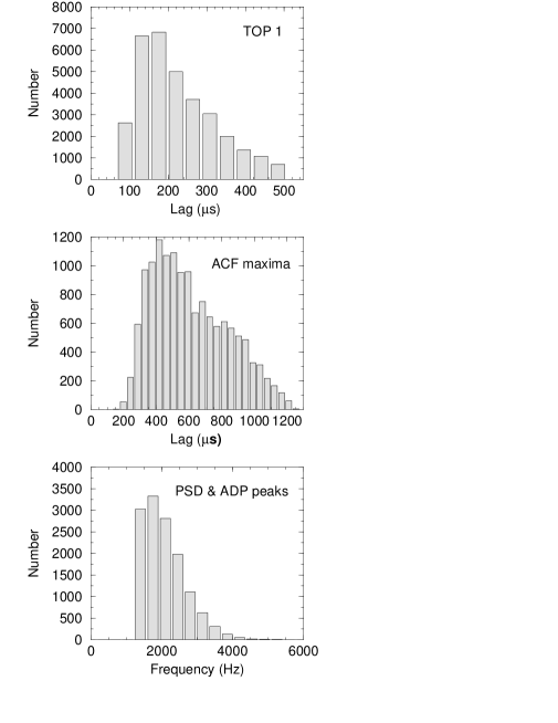
Figure 2: Results of the micro-structure analysis for 1.4 GHz. a) (top) Average pulse profile(s), average normalized ACF, (bottom) average PSD and average ADP, b) distributions derived from individual pulses as first order turn-off points in the ACF, first maxima in the ACF and first significant peaks simultaneously occurring in the PSD and ADP. For the mean pulse profiles in a) we show the average of all pulses (solid), the average of pulses exhibiting micro-structure (dashed) and the average of pulses without micro-structure (dotted).

At both frequencies we consistently detect micro-structure features in about 80% of all pulses. Hence, our results do not indicate that the micro-pulse component has a steeper spectrum as, for instance, inferred for PSR B2016+28 by Cordes et al. (1990). This is consistent with the finding of Lange et al. (1998) who detected micro-structure in virtually every pulsar strong enough to be observed at 4.85 GHz. We believe that previous reports on steeper spectra can be attributed to a limited signal-to-noise ratio available in those studies. Therefore, micro-structure appears to be a fundamental integral feature of pulsar radio emission.

Interestingly, we appear to detect a typical micro-structure time scale which is shorter at 2.3 GHz than at 1.4 GHz although the statistical significance is not very high. In order to test whether this is a result of the higher time resolution, we have performed our analysis on 2.3 GHz data modified to match the resolution at 1.4 GHz. We obtain the same result again, i.e. a smaller time scale at the higher frequency. In contrast, the determined periodicities are clearly identical within the errors and also agree among the different methods applied to obtain them. Hence, the micro-pulses may become narrower at 2.3 GHz but keep the same spacing if they appear in a quasi-periodic fashion. The fraction of micro-pulses for which we detect quasi-periodicities seems to be slightly smaller at the higher frequency. However, we cannot fully rule out a difference caused by a smaller signal-to-noise ratio at 2.3 GHz, or alternatively, by an effect described in the following.

In Figure 3 we show the average peak flux density of a micro-pulse at 2.3 GHz as a function of its width measured from the first turn-off point in the ACF. Those pulses for which we cannot identify a turn-off point and, hence, which are not identified to contain a micro-pulse of a certain width, are collected in the zero-th bin of this figure. This obviously happens typically for a micro-pulse width exceeding 250$\mu$s, which is identical to half of the quasi-periodicity (see Table 1). At this point, the micro-pulses obviously blend into each other and are not identified as separate entities any longer. The result of this effect and the increased peak flux density with larger micro-pulse width is the formation of significantly different pulse profiles when computed from those pulses for which we detect micro-structure and from those where we do not (see Fig. 2). While this effect confirms the determined average quasi-periodicity, it remains to be explained what causes the apparent correlation between micro-pulse peak flux density and width. In any case this interpretation suggests that the fraction of pulses containing micro-structure is even larger than the 80% we derive.

3.3 A temporal or radial origin of micro-structure?

Table 2 lists the pulsars which are known to have micro-structure. Comparing the micro-pulse separations, $P_{\mu}$, for different pulsars and frequencies, they seem to be frequency independent as previously summarized by Cordes et al. (1990). This is also true for the periodicities found for Vela at 1.4 GHz and 2.3 GHz as given in Table 1. The situation is, however, less clear for the micro-structure time-scale. Our Vela results may hint that micro-pulses may become narrower at higher frequencies, although this is not statistically significant and higher frequency data are needed. For other pulsars listed in Table 1 the uncertainties are often large – if multi-frequency data exist at all. The best studied case is PSR B1133+16, and there is indeed some indication that its time-scale is decreasing at higher frequencies: Hankins et al. (1976) reported a dependence of $\tau_{\mu}\propto\nu^{-0.22\pm 0.05}$ which is supported by the results of Ferguson & Seiradakis (1978). However, the compilation of PSR B1133+16 data in Table 1 makes these results less obvious, yielding a formal fit of $\tau_{\mu}\propto\nu^{-0.06\pm 0.10}$.

Table 2: Summary of previous micro-structure observations.

PSR B	Period	Freq.	$\tau_{\mu}$	$P_{\mu}$	Ref.
	(s)	(GHz)	($\mu$s)	($\mu$s)
0329+54	0.715	0.10	…	340	KKN78
		4.85	$<1500$	$600-1500$	LKWJ
0525+21	3.746	0.43	3000	…	COR79
0540+23	0.246	1.41	$<360$	…	LKWJ
0809+74	1.292	0.10	770	5000	CWH90
0823+26	0.531	0.43	550	…	COR79
		4.85	$300-700$	$360-660$	LKWJ
0834+06	1.273	0.43	1050	…	COR79
0950+08	0.253	0.11	100	400	CWH90
		0.11	200	…	RHC75
		0.32	200	…	RHC75
		0.43	100	400	CWH90
		0.43	170	…	CH77
		1.65	140	…	PBC01
		4.85	170	…	LKWJ
1133+16	1.188	0.10	500	…	PSS87
		0.10	500	…	PSS87
		0.10	574	…	HAN72
		0.20	651	…	HAN72
		0.32	525	…	HAN72
		0.43	340	…	CH77
		0.43	$130-200$	800	CWH90
		0.61	$130-200$	800	CWH90
		1.42	429	…	FGJ76
		1.65	$<10/300$	800/400	PBC01
		1.72	380	$180-1090$	FS78
		2.65	420	$180-1090$	FS78
		4.85	365	$<800$	LKWJ
1919+21	1.337	0.43	1300	…	COR79
1929+10	0.227	1.65	90	300	PBC01
		4.85	150	$240-1000$	LKWJ
1944+17	0.441	0.43	300	…	COR79
		0.43	160	800	CWH90
2016+28	0.558	0.32	160	800	CWH90
		0.43	290	900	COR76
		0.43	160	800	CWH90
		0.61	…	$500-750$	COR76
		0.61	160	800	CWH90
		1.41	160	800	CWH90
		1.41	240	640	LKWJ
2020+28	0.343	0.43	110	…	COR79

References: HAN72 - Hankins 1972, RHC75 - Rickett et al. 1975 COR76 - Cordes 1976, CH77 - Cordes & Hankins 1977, FGJ76 - Ferguson et al. 1976, FS78 - Ferguson & Seiradakis 1978, KKN78 - Kardashev et al. 1978, COR79 - Cordes 1979, PSS87 - Popov et al. 1987, CWH90 - Cordes et al. 1990, LKWJ - Lange et al. 1998, PBC01 - Popov et al. 2001

Figure 4 shows micro-pulse widths for different pulsars as a function of pulse period, $P$. We emphasize that this figures combines results derived at different frequencies (or averages of multi-frequency data if available for a given pulsar). This may introduce some scatter if a change in micro-pulse width with frequency is confirmed, but it is necessary to improve the otherwise small statistics. A similar plot using a smaller number of sources was presented by Cordes (1979) who suggested a linear dependence of $\tau_{\mu}$ on $P$. Obviously, this relationship still holds. The dashed line fitted to the data in Figure 4 corresponds to

$$\tau_{\mu}\;\mbox{($\mu$s)}=(600\pm 100)\;P\mbox{(s)}^{1.1\pm 0.2}$$ (1)

Interpreting such a linear dependence on period, one should be aware that the time resolution during observations usually scales similar, suggesting a possible instrumental origin of this result. We can reject such a possibility for our observations as we have analysed our data using different resolutions achieved by re-binning the data. Moreover, Popov et al. (2001) have studied micro-structure of PSR B1133+16 at 1.65 GHz with a resolution of only 62.5 ns. Although they find some features to be as short as 10$\mu$s, the vast majority of their detected micro-pulses show widths that are consistent which previous low resolution results, supporting a physical meaning of the above period trend.

Figure 3: Mean peak flux density as function of micro-pulse time scale as determined at 2.3 GHz. Peak flux densities were recorded for each analysis window along with determined time-scales. A width of zero indicates that no micro-pulse time scale was detected in the ACF.

In Fig. 4 we also show the time-scales determined for Vela’s micro-structure at 1.4 GHz and 2.3 GHz, respectively, which were not included in the fit leading to Eqn. (1). Including the data in the fit results in a $P^{0.9\pm 0.1}$–dependence (dotted line), i.e. making the slope only marginally flatter. Due to the typically large uncertainties, this fit is statistically not very different from Eqn. (1) (i.e. $\chi^{2}=3.4$ vs. $\chi^{2}=2.5$). While it would have interesting implications for the interpretation of micro-structure if the results for Vela indicated a flattening of the period relationship towards lower periods, such a conclusion is not justified given the current data. Observations of even faster rotating pulsars are required. In any case, however, it seems to be established that there is a clear period dependence of the width of normal micro-pulses, suggesting a temporal origin of micro-structure.

Finally, we note that giant micro-pulses are typically narrower than the normal ones, e.g. measuring the width (FWHM) of five giant micro-pulses with the largest S/N observed at 2.3 GHz, we obtain widths of 114 $\mu$s (338 Jy), 73 $\mu$s (213 Jy), 100 $\mu$s (100 Jy), 38 $\mu$s (232 Jy), 41 $\mu$s (172 Jy) with a typical uncertainty of 21 $\mu$s. Such widths would fit even better to Eqn. (1), which predicts a time-scale of about $40^{+40}_{-20}$ $\mu$s for Vela. However, we will argure later that giant micro-pulses may have a different origin to the normal micro-pulsars as, for example, we do not find any correlation between the strength and the width of giant micro-pulses.

Figure 4: Micro-structure time-scales derived for Vela at 1.4 GHz and 2.3 GHz, and time-scales reported for other pulsars as function of pulse period. The dashed line represents a best fit to all data but those determined for Vela. The dotted line is a fit including an averaged micro-pulse width for Vela.

4 Fluctuation analysis

A fluctuation analysis was carried out for the Vela pulsar by KD83. Their observations made at a frequency of 2.3 GHz was limited to an effective time resolution of 750 $\mu$s, i.e. a factor of 34 worse than our resolution at the same frequency. Two spectral features located at non-zero frequencies were found by KD83. In the trailing part of the pulse profile they identified a feature at 0.031 cycles period^-1 and in the right edge of the main pulse peak a broad spectral feature at 0.125 cycles period^-1.

Using our high resolution data, we have also performed a fluctuation spectra analysis in which we essentially follow the example of Backer (1970, 1973). Using continuous sets of individual pulses, we compute PSDs for the time series of pulse energy present in 50 adjacent windows covering the pulse profile in bins of 123 $\mu$s width each. Additionally, we calculate the PSD for the time series of an off-pulse window of the same size, which is subtracted from each of the on-pulse window PSDs. Usually, the power in each spectrum is normalized to match the power of the corresponding time series. However, in order to search for signals in weaker parts of the pulse profiles, we alternatively normalize the spectrum to a uniform RMS. In order to increase the signal-noise-ratio of spectral features at the cost of spectral resolution, we also compute the incoherent sum of power spectra obtained from Fast Fourier Transforms of smaller parts of the total available time series. Results are presented for 1.4 GHz and 2.3 GHz in Fig. 5. We find the same spectral features at both frequencies with a high degree of significance. Values for the pulse phase range, the determined centroid of the frequency feature and a frequency width estimated for a 10% level are listed in Table 3. Note that the features apparently existing at very small frequencies at phases $-$1.29 to 0.23 ms and 1.84 to 3.81 ms are consistent with zero frequency, similar to findings of KD83. Features 2 and 4 are obviously identical to those observed by KD83. Due to our better time resolution and sensitivity, we can however separate KD83’s second feature into three, apparently distinct features, here called 1, 2 and 3 (note the drop in power around these “frequency islands” in Fig. 5). We note that when comparing the determined centroids of these features, they seem to lie on a straight line with a slope of $0.025\pm 0.005$ (cycles period^-1) ms^-1. There are some indications that feature 2 is also visible in the longitude range of 1.82 to 1.93 ms, partly overlapping with feature 3. We performed an analysis as described by Deshpande & Rankin (2001) which shows that all three features represent the fundamental frequencies, i.e. they do not originate from higher frequencies being aliased due to the finite sampling once a period.

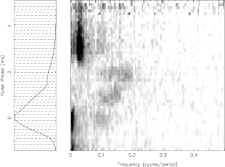
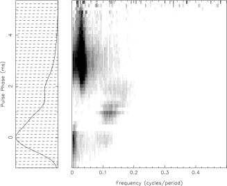
Figure 5: Average pulse profiles and fluctuation spectra computed from 12672 pulses at 1.4 GHz (left) and from 114688 pulses at 2.3 GHz (right). Four significant features at non-zero frequency are clearly visible.

Table 3: Spectral features derived from the fluctuation analysis. We quote the centre of the spectral feature, as well as their estimated width measured at a 10% level.

Pulse Phase Frequency Width S/N (ms) (cycles period^-1) (cycles period^-1) 1 $-0.30$ – 0.14 $0.093\pm 0.002$ $0.019\pm 0.002$ 4 2 0.68 – 1.13 $0.125\pm 0.003$ $0.031\pm 0.003$ 36 3 1.57 – 1.93 $0.134\pm 0.003$ $0.041\pm 0.004$ 8 4 1.48 – 4.52 $0.0335\pm 0.0004$ $0.0018\pm 0.0001$ 68

In Paper I we reported an extra profile feature, occurring sometimes as a strong “bump” component at the edge of the trailing profile, and speculated as to whether its appearance was periodic. Using our extremely long observation at 2.3 GHz, we can now rule out any significant periodicity for the occurrence of the bump, although the broad feature No. 4 listed in Table 3 partly covers this region.

5 Pulse Energy Distribution

The recent literature on the energy distribution of single pulses is rather sparse (except for those pulsars showing giant pulses). In Paper I we showed that the logarithm of the flux density of single pulses from the Vela pulsar had a Gaussian distribution (a so-called log-normal distribution). In retrospect, the distributions of single pulse energies shown in Ritchings (1976) and Hesse & Wielebinski (1974) for a variety of pulsars also appear to be log-normal although they are not discussed in that way by those authors. Cairns et al. (2001) showed that the phase-resolved intensity distributions also followed log-normal statistics in the Vela pulsar at 1.4 GHz. In this section we investigate different pulse phases at 2.3 GHz and examine their flux density distributions. Figure 6 shows the integrated pulse profile at 2.3 GHz, where we have picked out the strongest $\sim$2000 pulses showing the “bump” feature. Vertical lines mark the pulse phases of interest.

Figure 6: The integrated profile at 2.3 GHz of 2355 single pulses with flux densities greater than 5$\times$ the mean in the bump. The bump is visible as the trailing resolved peak of the profile. Dashed lines refer to pulse phases referred to in the text. The solid lines on the left denote the giant micro-pulse region, the pair on the right denote the bump region used in the analysis described in the text.

5.1 Main pulse window

We examined five phases (bins centred on the dashed lines in Fig. 6) equally spaced across the main pulse window. All of the flux density distribution of these bins can be fit with a log-normal distribution of pulse intensities convolved with a Gaussian noise distribution with constant mean 0.0 and sigma 2250 mJy. Table 4 summarises the means and sigmas of the fitted log-normal distributions. For illustration, Figure 7 shows the flux density distribution and cumulative probability distribution for phase 1.213 ms.

It is evident from the table that on the rising part of the pulse profile, the width of the distribution is large. This is the equivalent to saying that the modulation index in this part of the pulse is larger than that towards the middle of the pulse, which seems also to be the case in a number of pulsars. Also, these fits back up the idea that very large pulses in Vela arrive early, as pointed out by KD83. Cairns et al. (2001) discuss the implications for the emission mechanism of these log-normal distributions.

Table 4: Log-normal fits to the flux density distribution

Phase (ms)	Mean (Jy)	Sigma
$-$0.575	3.5	0.60
0.319	35.0	0.22
1.213	13.0	0.25
2.107	12.5	0.19
3.001	3.25	0.27

Figure 7: Histogram of energy distributions for phase 1.213 ms.

5.2 The bump region

We have attempted to isolate the bump component by choosing a window 42 bins wide indicated by the arrows on the right hand side shown Figure 6. We then computed the integrated flux density under these 42 bins for each of the 123,000 single pulses. Figure 8a shows the cumulative probability distribution along with the expected distribution from the instrumental response (which dominates the non-bump signal at these pulse phases). The presence of the bump component is clear in the figure but the form of its distribution less so. A power-law distribution overestimates the high flux probability. A log-normal distribution also does not fit the data well unless a cut-off is imposed at the low-flux end. This tends to suggest that the bump component results from a separate emitting entity.

Figure 8: Cumulative probability distribution of the integrated flux density under (a) the bump and (b) giant micro-pulse regions at 2.3 GHz. The curved lines show the distribution expected from Gaussian noise statistics which fits the data well at the low flux density end but not at the high end. An additional power-law component fits the data well in the right hand panel.

If the Vela pulsar consisted only of this component, its flux density would be $\sim$14 mJy. The distribution of flux densities shows that this component regularly has “giant pulses” with flux densities exceeding $10\times$ the mean flux density (Fig. 8a). There are 491 such pulses in the sample and so a giant pulse occurs every 250 rotations. These pulses contribute 17% of the total flux density in these phase bins. These are similar properties to the giant pulses seen in the Crab pulsar and it is tempting then also to relate the main pulse in Vela to the so-called pre-cursor in the Crab. Such a picture is not entirely convincing however, as the flux density distribution appears not to be a power-law. Moreover, there appears to be no coincidence between the location of any of the radio emission and the high energy emission from Vela, unlike the case of the Crab pulsar (see Moffett & Hankins 1999). The geometric viewing angles in the two cases are also rather different. In Vela the line of sight cuts close to the magnetic pole (Paper I) whereas in the Crab this angle is rather large [Moffett & Hankins 1999]. Additionally, Vela’s high energy emission is complex with the optical and soft X-ray emission occurring significantly later than the hard X-ray and $\gamma$-ray emission [Strickman, Harding & de Jager 1999]. Gouiffes (1998) has shown evidence for a component in the optical which is at the same phase as the peak of the radio emission. With only $\sim$1 ms time-resolution it is not clear whether any optical emission is associated with the radio bump component.

5.3 Giant micro-pulses

As previously discussed in Paper I, giant micro-pulses of emission are present at phases just prior to the main pulse. These are very sporadic, and have significant phase jitter of about 1 ms. We therefore chose a pulse window of about this size located at early phases as shown in Figure 6 to examine the flux density distribution of these micro-pulses. Figure 8b shows the cumulative probability distribution of the flux densities in these bins. It is evident that a power-law at high flux densities is necessary. The slope of the power law is $-2.85$, similar to that seen in both the Crab pulsar and PSR B1937+21. The occurrences of the giant micro-pulses are rather rare, only 60 pulses out of 123,000 form the power-law tail in the figure. Are the giant micro-pulses just an extension of the micro-structure pattern to outside the main pulse window or are they more related to the true giant pulses as seen in the Crab pulsar and PSR B1937+21? Assuming that Eqn. (1) is also valid for very small periods (cf. discussion in Section 3.3), one can estimate an expected micro-structure time-scale for PSR B1937+21. Interesting, the resulting time-scale of $\sim 0.5$ $\mu$s is coincident with the width measured for narrow (classical) giant pulses by Kinkhabwala & Thorsett (2000) at 1.4 GHz and 2.3 GHz. For the Crab pulsar the situation is more difficult. Its giant pulses often appear to be severely scattered, but Sallmen et al. (1999) report that any intrinsic time-scale of the pulse is unresolved at 0.6 GHz ($\la 10$ $\mu$s), while at 4.9 GHz pulse components are typically as short as 0.1 to 0.4 $\mu$s. This is much smaller than an extrapolated time-scale of 14$\mu$s.

In summary, the observed energy distribution of the giant micro-pulses bears similarities with that of known giant pulses (e.g. Romani & Johnston 2001). The giant micro-pulses tend to be narrower than the normal ones and, additionally, appear in a window outside that of the normal average profile. Hence, they may originate in the outer gap, as has been argued for the classical giant pulses (Romani & Johnston 2001), unlike the bulk of the radio emission.

6 Circular Polarization

As is well known, Vela shows a very high fraction of linear polarization at all pulse phases and for every pulse. Apart from the bump region, there are no orthogonal mode jumps at any pulse phase (KD83, Paper I). It is clear therefore, that one mode completely dominates in the Vela pulsar at all times; any other orthogonal mode, if present at all, must be less than $\sim$5% of the power of the dominant mode. The circular polarization of the integrated profile increases with increasing observing frequency and is about 15% at 2.3 GHz with a predominantly negative sign throughout the pulse. Individual pulses showing micro-structure appear to have circular polarization which is highly correlated with the total intensity. Occasionally the sign of circular polarization can be positive under a given micro-structure feature. A typical example of this is shown in Figure 9. Some micro-structure features are found to be greater than 90% circularly polarized which poses challenges to emission theories. It is important to re-iterate that change of the sign of the circular polarization is not accompanied by a orthogonal mode transition in the linear polarization (as is seen in other pulsars, see e.g. Cordes & Hankins 1977). This lack of mode transitions is not expected in the model of McKinnon & Stinebring (2000).

Figure 9: A single pulse in full polarization. The solid line denotes total intensity, dashed line linear polarization and dash-dotted line circular polarization. The top panel shows the position angle. Note the high degree of correlation between the total intensity and circular polarization and the sign reversal of the circular polarization under some components. Also note that the PA swing is not smooth but shows ’wiggles’ with typical time scales of a micro-pulse.

In order to study the relationship between total and circular intensity (Stokes $I$ and $V$) for the micro-pulses in more detail, we also performed the same micro-structure analysis on $V$ measured at 2.3 GHz. In contrast to the procedure described in Section 3.1, we used a fixed window of 128 phase bins centred on the central pulse peak. Consistent with the total power result summarized in Table 1, we detect micro-structure in $V$ in 83% of all measured pulses. The determined time scale $\tau_{\mu}$ of $87\pm 43$ $\mu$s is somewhat smaller than that for $I$ at the same frequency but just consistent within the uncertainties. We tentatively conclude that the micro-structure properties seen for $V$ are consistent with those seen in total power. This is similar to the result found in other pulsars by Cordes & Hankins (1977) and confirms the visual impression (see Fig. 9) that changes in the sign of the circular polarization occur at the edges of the micro-structure rather than the middle.

We also examined the distribution of flux densities of $V$ in a given phase bin. Indeed, we find that the distribution is again log-normal with the same value of sigma as for $I$ in the same phase bin. This is a remarkable result and implies that $V/I$ should be virtually constant from pulse to pulse in spite of large variations in flux. The distribution of $V/I$ is a Gaussian with a mean equal to the $V$ of the integrated profile and a sigma of 0.13. Figure 10 shows these distributions.

In spite of the excellent signal-to-noise ratio of the data, the distribution of $V/I$ is affected by noise. For example, when both $V$ and $I$ are low then $V/I$ is essentially random and this will cause a ‘pedestal’ in the distribution. When $V$ is close to zero this will cause an excess of counts near $V/I=0$ and the distribution may appear peakier than Gaussian. To quantify this effect we simulated the data in the following way. First we picked a value for $I$ from a log-normal distribution with a mean and sigma derived from the data as in Section 5.1. We then picked a random value for $V$ from a Gaussian distribution in $V/I$ with a mean equal to the integrated $V$ in that phase bin and a sigma ($\sigma_{v}$) which is a free parameter. Following this, Gaussian noise was added to both $I$ and $V$ (independently) and the ‘observed’ $V$, $I$, and $V/I$ were computed. This was repeated multiple times and the output distributions could then be compared with the real data.

We find that in the centre of the pulse, when $\sigma_{v}=0$, the resultant output distribution of $V/I$ has a width of 0.05. This is significantly less than the true distribution. We therefore find we need an intrinsic $\sigma_{v}$ of 0.11 to reproduce the observed data. As we go towards the edges of the pulse profile, the observed value of $\sigma_{v}$ becomes larger and larger. We find that virtually all of this increase can be explained by the decrease in signal-to-noise and that the underlying distribution of $\sigma_{v}$ is constant at 0.11.

Figure 10: Distribution of (top) total intensity, (middle) circular polarization and (bottom) percentage circular polarization for 25000 pulses at phase 0.32 ms.

7 Discussion

The origin of micro-structure is only one of the many questions still to be answered when studying pulsar radio emission. Micro-structure may be the product of either longitudinal modulation of the radiation pattern and/or caused by radial modulation of the emission or the creating plasma during the propagation in the magnetosphere. In any case, these and previous results indicate that micro-structure is an integral feature of pulsar emission that has to be explained together with the observed fluctuations and polarization.

Popov et al. (2001) found that the micro-pulse width of PSR B1133+16 scales with the width of the sub-pulse and the average component width, indicating that micro-structure may be related to the sweep of the beam. Interestingly, we find an obvious period dependence of the micro-pulse width which is a indeed good argument in favour of a temporal origin (i.e. sweeping of beams of emission) of micro-structure. The exact $\tau_{\mu}-P$ relationship and any possible break-down of such at very small periods will be probed by observing faster rotating pulsars and by studying Vela at an even higher frequency. If a change of micro-pulse width with frequency is indeed confirmed, we estimate that observations at 4.8 GHz should reveal a micro-structure width as predicted by Eqn. (1).

It is conceivable that the change in slope of the correlation of the micro-pulses’ peak flux density with their width shown in Figure 3 could be an artifact due to the finite sampling time. However, it could also indicate that there is an underlying population of superimposed and blended, even narrower micro-pulses with widths of typically 50 – 100 $\mu$s. Such narrow micro-pulses would be similar in width to the giant micro-pulses although they would not have similar peak flux densities, necessarily. However, if there is a population of narrow (normal) micro-pulses, it would be very difficult to explain why we still observe quasi-periodic micro-pulses with a preferred period – despite the blending. The preferred quasi-periodicity is even constant for different frequencies, while the observed average micro-pulse width is maybe not. Again, light can be shed on these questions if simultaneous multi-frequency observations of Vela micro-structure become available.

If confirmed, the decrease in the observed average width of a micro-pulse is stronger than but consistent with the general behaviour of the average pulse profiles (or even sub-pulses) which is often attributed to a Radius-to-Frequency mapping. If micro-structure represents micro-pulses emitted at a particular altitude sweeping our line-of-sight, we would indeed expect a smaller width at higher frequencies. The model of “micro-beams” creating the micro-pulses also finds support in the observations of “wiggles” in the position angle (PA) swing of the linearly polarized intensity. Compared to the very smooth average PA swing, that of individual pulses typically shows deviations from a average slope on time scales consistent with an average micro-pulse width, possibly relating these wiggles to PAs of separate micro-pulses (see Fig. 9). The quasi-periodicities may then be caused by a radial modulation of the emission. For instance, the spacing between separate micro-pulses may be determined by a radial distribution of emission patches, possibly arranged in a periodic way during the creation of the emitting plasma or modulations during propagation along the magnetic field lines. If that is the case, we would not necessarily expect a dependence of the quasi-periodicities, $P_{\mu}$, on rotation period unless the mechanism is directly dependent on the period value. Indeed, the data do not suggest any correlation between pulsar spin period and the quasi-periods observed in micro-pulses (see Table 2).

While we can conclude that normal micro-structure is an integral part of pulsar radio emission, in agreement with the results of Lange et al. (1998) and Popov et al. (2001), our study of the giant micro-pulses shows that these are different. They appear occasionally at pulse phases usually not covered by the normal pulses, have typically large amplitudes, appear to be narrower than normal micro-pulses, and also exhibit a power law in their cumulative probability distribution. All these properties strongly suggest that giant micro-pulses are a separate component of emission and more closely related to the classical giant pulses. The bump component is yet another facet which appears to be a separate feature that may also be related to giant pulses. Again, it appears only rarely and also exhibits a energy distribution that is not compatible with a log-normal distribution. As pointed out, if Vela consisted of only the bump component, it would regularly have classical giant pulses with a flux density exceeding the mean flux density by an order of magnitude. If classical giant pulses are related to high energy emission as suggested by Romani & Johnston (2001), and if giant micro-pulses and the bump are in turn related to giant pulses, then the absence of high-energy emission from these locations needs to be explained.

8 Summary

We have detected micro-structure in about 80% of all pulses, independent of frequency. Micro-pulses occurring in quasi-periodic fashion show the same separation at 1.4 and 2.3 GHz but may appear less frequently at the higher frequency. While there is a correlation between micro-pulse width and corresponding peak flux density, the width may decrease with frequency although this trend must be confirmed at higher frequencies. At 1.4 and 2.3 GHz, the micro-pulse width is somewhat larger than expected from extrapolation from other, slower rotating pulsars, although a period dependence is clearly visible. Narrower, giant micro-pulses which occur at pulse phases before the main pulse are indications of a possible relationship between giant micro-pulses and classical giant pulses. This is supported by our finding shown that the flux density distribution of the giant micro-pulses is best fitted by a power-law. All micro-pulses are highly linearly polarized and often show a large degree of circular polarization, with a strong correlation between Stokes $V$ and $I$. We find that phase-resolved intensity distribution are best fitted with log-normal statistics. We conclude that the “bump” component seems to be an extra component superposed on the main pulse

In summary, we find that Vela contains a mixture of emission properties representing both “classical” properties of radio pulsars and other radio features which are most likely related to high-energy emission. The Vela pulsar hence represents an ideal test case to study the relationship between radio and high-energy emission in significant detail.

References

- [Backer 1970] Backer D. C., 1970, Nature, 228, 752
- [Backer 1973] Backer D. C., 1973, ApJ, 182, 245
- [Boriakoff, Ferguson & Slater 1981] Boriakoff V., Ferguson D. C., Slater G., 1981, in Sieber W., Wielebinski R., eds, Pulsars, IAU Symposium 95. Reidel, Dordrecht, p. 199
- [Cairns, Johnston & Das 2001] Cairns I. H., Johnston S., Das P., 2001, ApJ, 563, L65
- [Cordes & Hankins 1977] Cordes J. M., Hankins T. H., 1977, ApJ, 218, 484
- [Cordes 1976] Cordes J. M., 1976, ApJ, 208, 944
- [Cordes 1979] Cordes J. M., 1979, Aust. J. Phys., 32, 9
- [Cordes, Weisberg & Hankins 1990] Cordes J. M., Weisberg J. M., Hankins T. H., 1990, AJ, 100, 1882
- [Craft, Comella & Drake 1968] Craft H. D., Comella J. M., Drake F., 1968, Nature, 218, 1122
- [Deshpande & Rankin 2001] Deshpande A. A., Rankin J. M., 2001, MNRAS, 322, 438
- [Drake & Craft 1968] Drake F. D., Craft H. D., 1968, Nature, 220, 231
- [Ferguson & Seiradakis 1978] Ferguson D. C., Seiradakis J. H., 1978, A&A, 64, 27
- [Ferguson et al. 1976] Ferguson D. C., Graham D. A., Jones B. B., Seiradakis J. H., Wielebinski R., 1976, Nature, 260, 25
- [Gouiffes 1998] Gouiffes C., 1998, in Shibazaki N., Kawai N., Shibata S., Kifune T., eds, Neutron Stars and Pulsars. Universal Academy Press, Inc., Tokyo, p. 363
- [Hankins & Rickett 1975] Hankins T. H., Rickett B. J., 1975, in Methods in Computational Physics Volume 14 — Radio Astronomy. Academic Press, New York, p. 55
- [Hankins 1971] Hankins T. H., 1971, ApJ, 169, 487
- [Hankins 1972] Hankins T. H., 1972, ApJ, 177, L11
- [Hankins 1996] Hankins T. H., 1996, in Johnston S., Walker M. A., Bailes M., eds, Pulsars: Problems and Progress, IAU Colloquium 160. Astronomical Society of the Pacific, San Francisco, p. 197
- [Hankins, Cordes & Rickett 1976] Hankins T. H., Cordes J. M., Rickett B. J., 1976, BAAS, 8, 10
- [Hesse & Wielebinski 1974] Hesse K. H., Wielebinski R., 1974, A&A, 31, 409
- [Jenet & Anderson 1998] Jenet F. A., Anderson S. B., 1998, PASP, 110, 1467
- [Jenet et al. 1997] Jenet F. A., Cook W. R., Prince T. A., Unwin S. C., 1997, PASP, 109, 707
- [Johnston & Romani 2002] Johnston S., Romani R., 2002, MNRAS, in press
- [Johnston et al. 2001] Johnston S., van Straten W., Kramer M., Bailes M., 2001, ApJ, 549, L101
- [Kardashev et al. 1978] Kardashev N. S. et al., 1978, SvA, 22, 583
- [Kinkhabwala & Thorsett 2000] Kinkhabwala A., Thorsett S. E., 2000, ApJ, 535, 365
- [Krishnamohan & Downs 1983] Krishnamohan S., Downs G. S., 1983, ApJ, 265, 372
- [Lange et al. 1998] Lange C., Kramer M., Wielebinski R., Jessner A., 1998, A&A, 332, 111
- [McKinnon & Stinebring 2000] McKinnon M. M., Stinebring D. R., 2000, ApJ, 529, 435
- [Moffett & Hankins 1999] Moffett D. A., Hankins T. H., 1999, ApJ, 522, 1046
- [Popov et al. 2001] Popov M. V., Bartel N., Cannon W. H., Novikov A. Y., Kondratiev V. I., Altunin V. I., 2001, A&A, submitted
- [Popov, Smirnova & Soglasnov 1987] Popov M. V., Smirnova T. V., Soglasnov V. A., 1987, SvA, 31, 529
- [Rickett, Hankins & Cordes 1975] Rickett B. J., Hankins T. H., Cordes J. M., 1975, ApJ, 201, 425
- [Ritchings 1976] Ritchings R. T., 1976, MNRAS, 176, 249
- [Romani & Johnston 2001] Romani R., Johnston S., 2001, ApJ, 557, L93
- [Strickman, Harding & de Jager 1999] Strickman M. S., Harding A. K., de Jager O. C., 1999, ApJ, 524, 373