Loop corrections to scalar quintessence potentials

Abstract

The stability of scalar quintessence potentials under quantum fluctuations is investigated for both uncoupled models and models with a coupling to fermions. We find that uncoupled models are usually stable in the late universe. However, a coupling to fermions is severely restricted. We check whether a graviton induced fermion-quintessence coupling is compatible with this restriction.

]

I Introduction

Observations indicate that dark energy constitutes a substantial fraction of our Universe [1, 2, 3, 4, 5]. The range of possible candidates includes a cosmological constant and – more flexibly – some form of dark energy with a time dependent equation of state, called quintessence [6]. Commonly, realizations of quintessence scenarios feature a light scalar field [7, 8, 9].

The evolution of the scalar field is usually treated at the classical level. However, quantum fluctuations may alter the classical quintessence potential. In this article, we will investigate one-loop contributions to the effective potential from both quintessence and fermion fluctuations. We will show that in the late universe, quintessence fluctuations are harmless for most of the potentials used in the literature. For inverse power laws and SUGRA inspired models, this has already been demonstrated in [10]. That the smallness of the quintessence mass needs to be protected by some symmetry has been pointed out in [11, 12].

In contrast with the rather harmless quintessence field fluctuations, fermion fluctuations severely restrict the magnitude of a possible coupling of quintessence to fermionic dark matter, as we will show.

In Euclidean conventions, the action we use for the quintessence field $\Phi$ and a fermionic species $\Psi$ to which it may couple [13, 14, 15] is

$$S=\int d^{4}x\ \sqrt{g}\Bigg{[}\textrm{M}_{\textrm{P}}^{2}R+\mathinner{1\over 2}\partial_{\mu}\Phi(x)\partial^{\mu}\Phi(x)+V(\Phi(x))\\ +\bar{\Psi}(x)\left[i\ /\!\!\!\!\nabla+\gamma^{5}m_{\rm f}(\Phi)\right]\Psi(x)\Bigg{]},$$ (1)

with $m_{\rm f}(\Phi)$ as a $\Phi$ dependent fermion mass. This $\Phi$ dependence (if existent in a model) determines the coupling of the quintessence field to the fermions. As long as one is not interested in quantum gravitational effects, one may set $\sqrt{g}=1$, $R=0$ and replace $/\!\!\!\!\nabla\rightarrow/\!\!\!\partial$ in the action (1).

By means of a saddle point expansion [16], we arrive at the effective action $\Gamma[\Phi_{\rm cl}]$ to one loop order of the quintessence field. The equation governing the dynamics of the quintessence field is then determined by $\delta\Gamma[\Phi_{\rm cl}]_{|\Phi_{\rm cl}=\Phi_{\rm cl}^{\star}}=0$. When estimating the magnitude of the loop corrections, we will assume that $\Phi_{\rm cl}^{\star}$ is close to the solution of the classical field equations: $\delta S=0$. Evaluating $\Gamma$ for constant fields, we can factor out the space-time volume $U$ from $\Gamma=UV$. This gives the effective potential

$$V_{\textrm{{1-loop}}}^{\textsc{}}(\Phi_{\rm cl})=V(\Phi_{\rm cl})+\mathinner{\Lambda^{2}\over 32\pi^{2}}V^{\prime\prime}(\Phi_{\rm cl})-\mathinner{\Lambda_{\rm ferm}^{2}\over 8\pi^{2}}\left[m_{\rm f}(\Phi_{\rm cl})\right]^{2}.$$ (2)

Here, primes denote derivatives with respect to $\Phi$; $\Phi_{\rm cl}$ is the classical field value and $\Lambda$ and $\Lambda_{\rm ferm}$ are the ultra violet cutoffs of scalar and fermion fluctuations. The last term in Equation (2) accounts for the fermionic loop corrections as shown in figure 3. The second term in Equation (2), is the leading order scalar loop, depicted in figure 1. We neglect graphs of the order $(V^{\prime\prime}_{|\rm cl})^{2}$ and higher like the one in figure 1, because $V$ and its derivatives are of the order $10^{-120}$ (see section III). We have also ignored $\Phi$-independent contributions, as these will not influence the quintessence dynamics.

FIG. 1.: Pure quintessence fluctuations (depicted as dashed lines). The loop of the fluctuating quintessence field modifies the potential. Since the potential involves in principle arbitrary powers of $\Phi$, we depict $V^{\prime\prime}$ as multiple external lines.

However, the $\Phi$-independent contributions add up to a cosmological constant of the order $\Lambda^{4}\approx{\mathcal{O}}(\textrm{M}_{\textrm{P}}^{4})$. This is the old cosmological constant problem, common to most field theories. We hope that some symmetry or a more fundamental theory will force it to vanish. The same symmetries or theories could equally well remove the loop contribution by some cancelling mechanism. After all, this mechanism must be there, for the observed cosmological constant is far less than the naively calculated ${\mathcal{O}}(\textrm{M}_{\textrm{P}}^{4})$. Unfortunately, SUSY is broken too badly to be this symmetry [11].

In addition, none of the potentials under investigation can be renormalized in the strict sense. However, as we will see, terms preventing renormalization may in some cases be absent to leading order in $V^{\prime\prime}_{|\rm cl}$. As the mass of the quintessence field is extremely small, one may for all practical purposes view these specific potentials (such as the exponential potential) as renormalizable.

There is also a loophole for all models that will be ruled out in the following: The potential used in a given model could be the full effective potential including all quantum fluctuations, down to macroscopic scales. For coupled quintessence models, this elegant argument is rather problematic and the loophole shrinks to a point (see section III).

In the following, we apply Equation (2) to various quintessence models in order to check their stability against one loop corrections. We do this separately for coupled and uncoupled models. We use units in which $\textrm{M}_{\textrm{P}}=1$. For clarity, we restore it when appropriate.

II Uncoupled quintessence

Here, we are going to discuss inverse power law, pure and modified exponential, and cosine-type potentials.

A Inverse power law and exponential potentials

Inverse power laws [7, 8], exponential potentials [9, 17] and mixtures of both [18] can be treated by considering the potential $V=A\Phi^{-\alpha}\exp(-\lambda\Phi^{\gamma})$ [19]. Limiting cases include inverse power laws, exponentials, and SUGRA inspired models. Deriving twice with respect to $\Phi$, we find

$$V^{\prime\prime}=A\Phi^{-\alpha}\exp(-\lambda\Phi^{\gamma})\Bigl{\{}\alpha(\alpha+1)\Phi^{-2}+2\alpha\lambda\gamma\Phi^{\gamma-2}\\ +\lambda^{2}\gamma^{2}\Phi^{2\gamma-2}-\lambda\gamma(\gamma-1)\Phi^{\gamma-2}\Bigr{\}}.$$ (3)

1 Inverse power laws

For inverse power laws, we set $\gamma=\lambda=0$. This gives the classical potential $V_{\textrm{cl}}^{\textsc{ipl}}=A\Phi_{\rm cl}^{-\alpha}$ and by means of Equation (2) the loop corrected potential

$$V_{\textrm{{1-loop}}}^{\textsc{ipl}}=V_{\textrm{cl}}^{\textsc{ipl}}\left(1+\mathinner{1\over 32\pi^{2}}\Lambda^{2}\alpha(\alpha+1)\Phi_{\rm cl}^{-2}\right).$$ (4)

The potential is form stable if $\mathinner{1\over 32\pi^{2}}\Lambda^{2}\alpha(\alpha+1)\Phi^{-2}\ll 1$, which today is satisfied, as $\Phi\approx\textrm{M}_{\textrm{P}}$ [18].

However, if the field is on its attractor today, then $\Phi\propto(1+z)^{-3/(\alpha+2)}$, where $z$ is the redshift [18]. Using this, we have for $z\gg 1$

$$V_{\textrm{{1-loop}}}^{\textsc{ipl}}\approx V_{\textrm{cl}}^{\textsc{ipl}}\left(1+\mathinner{1\over 32\pi^{2}}\Lambda^{2}\alpha(\alpha+1)z^{6/(\alpha+2)}\right).$$ (5)

Thus, the cutoff needs to satisfy $\Lambda^{2}\ll\mathinner{32\pi^{2}\over\alpha(\alpha+1)}\times z^{-6/(\alpha+2)}$. Cosmologically viable inverse power law potentials seem to be restricted to $\alpha<2$ [20, 21]. Using $\alpha=1$ and $z\approx 10^{4}$ for definiteness, the bound becomes $\Lambda^{2}\ll 10^{-6}$.

So, at equality (and even worse before that epoch), the cutoff needs to be well below $10^{12}$ Gev, if classical calculations are meant to be valid. In [10] it is argued that for inverse power laws, the quintessence content in the early universe is negligible and hence the fluctuation corrections are important only at an epoch where quintessence is subdominant. As the loop corrections introduce only higher negative powers in the field, it is hoped that, even though one does not know the detailed dynamics, the field will nevertheless roll down its potential (which at that time is supposed to be much steeper) and by the time it is is cosmologically relevant, the classical treatment is once again valid. Having no means of calculating the true effective potential for the inverse power law in the early universe, this view is certainly appealing.

2 Pure exponential potentials

The pure exponential potential is special because its derivatives are multiples of itself. The classical potential (with $\alpha=0,\ \gamma=1$) is $V_{\textrm{cl}}^{\textsc{ep}}=A\exp(-\lambda\Phi_{\rm cl})$ and to one loop order

$$V_{\textrm{{1-loop}}}^{\textsc{ep}}=V_{\textrm{cl}}^{\textsc{ep}}\left\{1+\mathinner{1\over 32\pi^{2}}\Lambda^{2}\lambda^{2}\right\}.$$ (6)

It is easy to see that a rescaling of $A\to A/\left(1+\mathinner{1\over 32\pi^{2}}\Lambda^{2}\lambda^{2}\right)$ absorbs the loop correction, leading to a stable potential up to order $V_{\rm cl}^{\prime\prime}$. Working to next to leading order, i.e. restoring terms of order $(V_{\rm cl}^{\prime\prime})^{2}$, we get

$\displaystyle V_{\textrm{{1-loop},\, n.l.}}^{\textsc{ep}}=\mathinner{1\over 32\pi^{2}}\left(V_{\rm cl}^{\prime\prime}\right)^{2}\ln\left(\mathinner{V_{\rm cl}^{\prime\prime}\over\Lambda^{2}}\right).$

It is this term which in four dimensions spoils strict renormalizability.

B Nambu-Goldstone cosine potentials

Cosine type potentials resulting from a quintessence axion were introduced in [22, 23] and their implications for the CMB have been studied in [24]. They take on the classical potential $V_{\textrm{cl}}^{\textsc{ng}}=A\left[1-\cos\left(\Phi_{\rm cl}/f_{Q}\right)\right]$ and including loop corrections

$\displaystyle V_{\textrm{{1-loop}}}^{\textsc{as}}=A\left[1-\left\{1-\mathinner{1\over 32\pi^{2}}\mathinner{\Lambda^{2}\over f_{Q}^{2}}\right\}\cos\left(\mathinner{\Phi_{\rm cl}\over f_{Q}}\right)\right].$

Upon a redefinition $A\to A/\left\{1-\mathinner{1\over 32\pi^{2}}\mathinner{\Lambda^{2}\over f_{Q}^{2}}\right\}$ and, recalling that the loop correction is only defined up to a constant, one arrives at the same functional form as the classical potential.

C Modified exponentials

In the model proposed by Albrecht and Skordis [25], the classical potential is $V_{\textrm{cl}}^{\textsc{as}}=V_{p}\exp(-\lambda\Phi_{\rm cl})$, where $V_{p}$ is a polynomial in the field. To one loop order, this leads to

$$V_{\textrm{{1-loop}}}^{\textsc{as}}=V_{\textrm{cl}}^{\textsc{as}}\left\{1+\mathinner{1\over 32\pi^{2}}\Lambda^{2}\left(\mathinner{V_{p}^{\prime\prime}\over V_{p}}-2\lambda\mathinner{V_{p}^{\prime}\over V_{p}}+\lambda^{2}\right)\right\}.$$ (7)

Let us for definiteness discuss the example given in [25], where the authors chose $V_{p}(\Phi)=(\Phi-B)^{2}+C$. With this choice, we have

$$V_{\textrm{{1-loop}}}^{\textsc{as,\,exmpl}}=V_{\textrm{cl}}^{\textsc{as,\,exmpl}}\bigg{\{}1+\mathinner{1\over 32\pi^{2}}\Lambda^{2}\Big{(}\mathinner{1\over V_{p}}\big{[}2\\ -4\lambda(\Phi_{\rm cl}-B)\big{]}+\lambda^{2}\Big{)}\bigg{\}}.$$ (8)

Now consider field values close to the minimum of $V_{p}$, i.e., let the absolute value of $\xi\equiv\Phi_{\rm cl}-B$ be small compared to $\sqrt{C}$. Then

$$V_{\textrm{{1-loop}}}^{\textsc{as,\,exmpl}}=V_{\textrm{cl}}^{\textsc{as,\,exmpl}}\left\{1+\mathinner{\Lambda^{2}\over 32\pi^{2}}\left(\mathinner{2-4\lambda\xi\over C+\xi^{2}}+\lambda^{2}\right)\right\},$$ (9)

and to leading order in $\xi$

$$V_{\textrm{{1-loop}}}^{\textsc{as,\,exmpl}}\approx V_{\textrm{cl}}^{\textsc{as,\,exmpl}}\left\{1+\mathinner{\Lambda^{2}\over 32\pi^{2}}\left(\mathinner{1\over C}\left[2-4\lambda\xi\right]+\lambda^{2}\right)\right\}.$$ (10)

Now consider, as was the case in the example given in [25], $C=0.01$ for definiteness. If we assume a cutoff $\Lambda$ and a Plank mass of approximately the same order, we get

$$V_{\textrm{{1-loop}}}^{\textsc{as,\,exmpl}}\approx V_{\textrm{cl}}^{\textsc{as,\,exmpl}}\left\{1+\mathinner{1\over 32\pi^{2}}\left(100\left[2-4\lambda\xi\right]+\lambda^{2}\right)\right\}.$$ (11)

The $\xi$ (and hence $\Phi_{\rm cl}$) dependent contribution in the curly brackets of Equation (11) is $-25/(2\pi^{2})\lambda\xi$ which for the value $\lambda=8$ chosen in the example gives $-200/(2\pi^{2})\xi\approx-10\xi$.

If we now look at the behaviour of the loop correction as a function of $\Phi_{\rm cl}$ and hence $\xi$ in the vicinity of the minimum of this example polynomial, we see that for, e.g., $\xi=0.01$, the one loop contribution dominates the classical potential giving rise to a linear term in $\Phi_{\rm cl}$ unaccounted for in the classical treatment. For many values of the parameters $B$ and $C$, this just changes the form and location of the bump in the potential. In principle, however the loop correction can remove the local minimum altogether (see figure 2).

Needless to say that this finding depends crucially on the cutoff. If it is chosen small enough, the conclusion is circumvented. In addition, only the specific choice of $V_{p}$ above has been shown to be potentially unstable. The space of polynomials is certainly large enough to provide numerous stable potentials of the Albrecht and Skordis form.

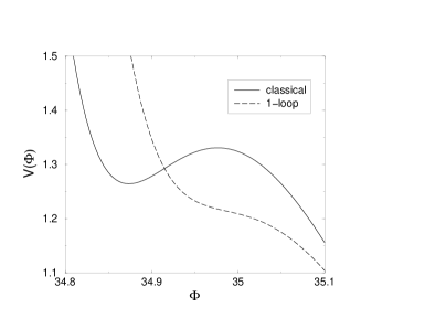
FIG. 2.: Classical and 1-loop corrected potential [in $10^{-123}\textrm{M}_{\textrm{P}}^{4}$] for $V_{\textrm{cl}}^{\textsc{as}}=\left[(\Phi-B)^{2}+C\right]\exp(-\lambda\Phi_{\rm cl})$ with $B=34.8,\ C=0.013,\ \Lambda=1.2$. The classical potential has a local minimum, which is absent for the loop corrected one. This is a hand-picked example and in most cases, the bump will not vanish but move and change its form.

III Coupled quintessence

Various models featuring a coupling of quintessence to some form of dark matter have been proposed [26, 14, 27, 28, 15]. From the action Equation (1), we see that the mass of the fermions could be $\Phi$ dependent: $m_{\rm f}=m_{\rm f}(\Phi_{\rm cl})$. Two possible realization of this mass dependence are, for instance, $m_{\rm f}=m^{0}_{\rm f}\exp(-\beta\Phi_{\rm cl})$ and $m_{\rm f}=m^{0}_{\rm f}+c(\Phi_{\rm cl})$, where in the second case, we may have a large field independent part together with small couplings to quintessence. For the model discussed in [14], the coupling is of the first form, whereas in [15], the coupling is realized by multiplying the cold dark matter Lagrangian by a factor $f(\Phi$). This factor is usually taken of the form $f(\Phi)=1+\alpha(\Phi-\Phi_{0})^{\beta}$. Hence, the coupling is $m_{\rm f}(\Phi)=f(\Phi)\,m_{\rm f}^{0}$, if we assume that dark matter is fermionic. If it were bosonic, the following arguments would be similar.

We will first discuss general bounds on the coupling and in a second step check whether these bounds are broken via an effective gravitational coupling.

A General bounds on a coupling

We will discuss only the new effects coming from the coupling and set

$$V_{\textrm{{1-loop}}}^{\textsc{}}=V_{\textrm{cl}}^{\textsc{}}-\Delta V,$$ (12)

where $\Delta V=\Lambda_{\rm ferm}^{2}\left[m_{\rm f}(\Phi_{\rm cl})\right]^{2}/\left(8\pi^{2}\right)$. If we assume that the potential energy of the quintessence field constitutes a considerable part of the energy density of the universe today, i.e. $\rho_{\rm q}\sim\rho_{\rm critical}$, we see from the Friedmann equation

$$3H^{2}=\rho_{\rm critical},$$ (13)

that $V_{\textrm{cl}}^{\textsc{}}\sim H^{2}$. With today’s Hubble parameter $H=8.9\times 10^{-61}\,h$ ($h=0.5\dots 0.9$), we have

$$V_{\rm cl}\sim 7.9\times 10^{-121}\,h^{2}.$$ (14)

The ratio of the ‘correction’ to the classical potential is

$$\mathinner{\Delta V\over V_{\textrm{cl}}^{\textsc{}}}=\mathinner{1\over 8\pi^{2}}\mathinner{\Lambda_{\rm ferm}^{2}\left[m_{\rm f}(\Phi_{\rm cl})\right]^{2}\over V_{\textrm{cl}}^{\textsc{}}}.$$ (15)

Let us first consider the case that all of the fermion mass is field dependent, i.e., we consider cases like $m_{\rm f}=m^{0}_{\rm f}\exp(-\beta\Phi_{\rm cl})$. As an example, we choose a fermion cutoff at the GUT scale $\Lambda_{\rm ferm}=10^{-3}$, and a fermion mass, $m_{\rm f}(\Phi_{\rm cl})$ of the order of $100\,\textrm{Gev}=10^{-16}\textrm{M}_{\textrm{P}}$. Then Equation (15) gives the overwhelmingly large ratio

$$\mathinner{\Delta V\over V_{\textrm{cl}}^{\textsc{}}}\approx 10^{80}.$$ (16)

Thus, the classical potential is negligible relative to the correction induced by the fermion fluctuations.

Having made this estimate, it is clear that the fermion loop corrections are harmless only, if the square of the coupling takes on exactly the same form as the classical potential itself. If, for example, we have an exponential potential $V_{\textrm{cl}}^{\textsc{}}=A\exp(-\lambda\Phi_{\rm cl})$ together with a coupling $m_{\rm f}(\Phi_{\rm cl})=m^{0}_{\rm f}\exp(-\beta\Phi_{\rm cl})$, then this coupling can only be tolerated, if $2\beta=\lambda$. Taken at face value, this finding restricts models with these types of coupling. It is however interesting to note that for exponential coupling, the case $2\beta=\lambda$ is not ruled out by cosmological observations [28].

Turning to the possibility of a fermion mass that consists of a field independent part and a coupling, i.e., $m_{\rm f}=m^{0}_{\rm f}+c(\Phi_{\rm cl})$, Equation (15) becomes

$$\mathinner{\Delta V\over V_{\textrm{cl}}^{\textsc{}}}=\mathinner{1\over 8\pi^{2}}\mathinner{\Lambda_{\rm ferm}^{2}\left[2m^{0}_{\rm f}c(\Phi_{\rm cl})+c(\Phi_{\rm cl})^{2}\right]\over V_{\textrm{cl}}^{\textsc{\,}}},$$ (17)

where we have ignored a quintessence field independent contribution proportional to $(m^{0}_{\rm f})^{2}$. Assuming $c(\Phi_{\rm cl})\ll m^{0}_{\rm f}$, and demanding that the loop corrections should be small compared to the classical potential, Equation (17) yields the bound

$$c(\Phi_{\rm cl})\ll\mathinner{4\pi^{2}\,V_{\textrm{cl}}^{\textsc{\,}}\over\Lambda_{\rm ferm}^{2}m^{0}_{\rm f}}.$$ (18)

If, as above, we assume $\Lambda_{\rm ferm}=10^{-3}\textrm{M}_{\textrm{P}}$, $m^{0}_{\rm f}=10^{-16}\textrm{M}_{\textrm{P}}$ and $V_{\textrm{cl}}^{\textsc{}}$ from Equation (14), this gives

$$c(\Phi_{\rm cl})\ll 3\times 10^{-97},$$ (19)

in units of the Planck mass. Once again, the bound from Equation (18) applies only if the functional form of the loop correction differs from the classical potential. Assuming a Yukawa-type coupling $c(\Phi_{\rm cl})=\beta\Phi_{\rm cl}$ and field values of at least the order of the Plank mass, we get $\beta\ll 10^{-97}$.

For the coupling $c(\Phi)=m_{\rm f}^{0}\alpha(\Phi-\Phi_{0})^{\beta}$ with the values $\alpha=50,\,\beta=8,\,\Phi_{0}=32.5$ given in [15], $c(\Phi)$ is usually larger than $m_{\rm f}^{0}$. Therefore we take $m_{\rm f}(\Phi_{\rm cl})\approx c(\Phi_{\rm cl})$. With $m_{\rm f}(\Phi_{\rm cl})=10^{-16}$ as before, we get the same result as in (16).

FIG. 3.: Correction to the quintessence potential due to fermion fluctuations. Fermion lines are solid, quintessence lines dashed. Shown is the case where $m_{\rm f}(\Phi)$ gives a Yukawa coupling, i.e. $c(\Phi)=\beta\Phi$, corresponding to one quintessence line. Of course, for more complicated $m_{\rm f}(\Phi)$ such as $m_{\rm f}(\Phi_{\rm cl})=m^{0}_{\rm f}\exp(-\beta\Phi_{\rm cl})$, several external lines as in figure 1 would appear.

The coupled models share one property: the loop contribution from the coupling is by far larger than the classical potential. At first sight, the golden way out of this seems to be to view the potential as already effective: all fluctuations would be included from the start. However, there is no particular reason, why any coupling of quintessence to dark matter should produce just exactly the effective potential used in a particular model: there is a relation between the coupling and the effective potential generated. Put another way, if the effective potential is of an elegant form and we have a given coupling, then it seems unlikely that the classical potential could itself be elegant or natural.

B Effective gravitational fermion quintessence coupling

FIG. 4.: Effective fermion-quintessence coupling via graviton exchange. The fermions (solid lines) emit gravitons (wiggled lines) which are caught by the quintessence field (dashed lines). As the graphs involve couplings of the gravitons to the classical quintessence potential, the generated coupling is proportional to the classical potential. Since the potential involves arbitrary powers of $\Phi$, we depict it as several $\Phi$-lines. A Yukawa type coupling, corresponding to just one line, is then generated by power expanding $V(\Phi)=V(\Phi_{\rm cl}){}+V_{|\textrm{cl}}^{\prime}\,(\Phi-\Phi_{\rm cl})$ in the fluctuating field.

The bound in Equation (18) is so severe that the question arises whether gravitational coupling between fermions and the quintessence field violates it. To give an estimate, we calculate two simple processes depicted in figure 4. We evaluate the diagrams for vanishing external momenta. This is consistent with our derivation of the fermion loop correction Equation (2), in which we have assumed momentum independent couplings. The effective coupling due to the graviton exchange contributes to the fermion mass, which becomes $\Phi_{\rm cl}$ dependent. We assume that this coupling is small compared to the fermion mass and write $m_{\rm f}(\Phi_{\rm cl})=m_{\rm f}^{0}+c(\Phi_{\rm cl})$.

From the first diagram, figure 4 we get (see the Appendix A):

$$c(\Phi_{\rm cl})=\mathinner{1\over 8\pi^{2}}m_{\textrm{f}}^{0}V(\Phi_{\rm cl})\times\Bigg{[}\ln\left(\mathinner{\Lambda^{2}\over\Lambda^{2}+\left[m_{\rm f}^{0}\right]^{2}}\right)\\ -\ln\left(\mathinner{\lambda^{2}\over\lambda^{2}+\left[m_{\rm f}^{0}\right]^{2}}\right)\Bigg{]},$$ (20)

whereas 4 gives

$$c(\Phi_{\rm cl})=\mathinner{5\over 8\pi^{2}}m_{\textrm{f}}^{0}V(\Phi_{\rm cl})\ln\left(\mathinner{\Lambda\over\lambda}\right).$$ (21)

Here, we have introduced infrared and ultraviolet cutoffs $\lambda$ and $\Lambda$ for the graviton momenta. We assume $\Lambda$ to be of the order $\textrm{M}_{\textrm{P}}$ and $\lambda$ about the inverse size of the horizon. Since the results depend only logarithmically on the cutoffs, this choice is not critical, and in addition $\ln(\textrm{M}_{\textrm{P}}/H)\approx 140$, which is small. From Equation (17, 21, 20), we see that, in leading order, the change in the quintessence potential due to this effective fermion coupling would be proportional to $V(\Phi_{\rm cl})$ and could hence be absorbed upon redefining the pre-factor of the potential (see also figure 5). In next to leading order, the contribution is proportional to $V(\Phi_{\rm cl})^{2}$, which is negligible.

From the Appendix A, in which we present the calculation in more detail, it is clear that there are processes where the vertices are more complicated. However, to this order all diagrams are proportional to $V(\Phi_{\rm cl})$. Thus, they can be absorbed just like the two processes presented above.

FIG. 5.: Fermion loop contribution to the quintessence potential involving the effective coupling figure 4. The cross in the fermion line depicts the field independent fermion mass $m_{\rm f}^{0}$.

IV Weyl transformed fields

So far, we have assumed a constant Planck mass together with a field independent cutoff. We could, however, assume that the Planck mass is not constant, but rather given by the expectation value of a scalar field $\chi$. We will call the frame resulting from this Weyl scaling the Weyl frame, as opposed to the frame with a constant Plank mass which we will call the Einstein frame. From the classical point of view, both frames are equivalent. On calculating quantum corrections, we have to evaluate a functional integral. Usually, the functional measure in the Einstein frame is set to unity. In principle, the variable change associated with the Weyl scaling leads to a non-trivial Jacobian and therefore a different functional measure. Taking the position that the Weyl frame is fundamental, this measure could equally well be set to unity in the Weyl frame. Therefore, it is a priori unclear whether the loop corrected potential in the Weyl frame, when transformed back into the Einstein frame, will be the same as the one from Equation (2).

As the cutoff in the Einstein frame is a constant mass scale and hence proportional to the Plank mass, it seems natural to assume that the cutoff in the Weyl frame is proportional to $\chi$. We restrict our discussion to this case. For other choices of the $\chi$-dependence of the cutoff, the results may differ.

The Weyl transformation is achieved by scaling the metric, the curvature scalar, all fields, and the tetrad by appropriate powers of $\chi/\textrm{M}_{\textrm{P}}$ (see table I) [9, 26]:

$$\tilde{S}=\int d^{4}x\sqrt{\tilde{g}}\Bigg{[}\chi^{2}\tilde{R}+\mathinner{z\over 2}\partial_{\mu}\chi\partial^{\mu}\chi+W(\chi)\\ +\tilde{\bar{\Psi}}\left(i\,\tilde{\gamma}^{\mu}(x)\nabla_{\mu}+\chi\mathinner{m_{\rm f}(\Phi_{\rm cl})\over\textrm{M}_{\textrm{P}}}\gamma^{5}-\mathinner{3\over 2}i\tilde{\gamma}^{\mu}(x)\ln\chi_{,\mu}\right)\tilde{\Psi}\Bigg{]},$$ (22)

where $\Phi=(12+z)^{1/2}\textrm{M}_{\textrm{P}}\ln(\chi/\textrm{M}_{\textrm{P}})$ and

$$W(\chi)\equiv\left(\mathinner{\chi\over\textrm{M}_{\textrm{P}}}\right)^{4}V(\Phi(\chi)).$$ (23)

The term proportional to $\ln\chi_{,\mu}$ in Equation (22) is somewhat inconvenient. Adopting the position that the Weyl frame is fundamental, this term is unnatural. Instead, one could formulate the theory with canonical couplings for the fermions. Dropping this term,

$$\tilde{S}_{\textrm{can.}}=\int d^{4}x\sqrt{\tilde{g}}\Bigg{[}\chi^{2}\tilde{R}+\mathinner{z\over 2}\partial_{\mu}\chi\partial^{\mu}\chi+W(\chi)\\ +\tilde{\bar{\Psi}}\left(i\,\tilde{\gamma}^{\mu}(x)\nabla_{\mu}+\mathinner{\chi\over\textrm{M}_{\textrm{P}}}m_{\rm f}(\Phi(\chi))\,\gamma^{5}\right)\tilde{\Psi}\Bigg{]},$$ (24)

we observe by going back to the usual action $\tilde{S}_{\textrm{can.}}\to S$,

$$S=\int d^{4}x\ \sqrt{g}\Bigg{[}\mathinner{1\over 2}\partial_{\mu}\Phi(x)\partial^{\mu}\Phi(x)+V(\Phi(x))\\ +\bar{\Psi}(x)\left(i/\!\!\!\!\nabla+\gamma^{5}m_{\rm f}(\Phi)+\mathinner{3\over 2\textrm{M}_{\textrm{P}}}i\,\gamma^{\mu}(x)\phi_{,\mu}\right)\Psi(x)\Bigg{]},$$ (25)

that the canonical form of the action in the Weyl frame gives rise to a derivative coupling of the quintessence field to the fermions in the Einstein frame, which we can safely ignore.

$g_{\mu\nu}$ $\to$	$(\chi/\textrm{M}_{\textrm{P}})^{2}\,\tilde{g}_{\mu\nu}$
$g^{\mu\nu}$ $\to$	$(\chi/\textrm{M}_{\textrm{P}})^{-2}\,\tilde{g}^{\mu\nu}$
$\sqrt{g}$ $\to$	$(\chi/\textrm{M}_{\textrm{P}})^{4}\,\sqrt{\tilde{g}}$
$R$ $\to$	$\left(\chi/\textrm{M}_{\textrm{P}}\right)^{-2}\left(\tilde{R}-6\tilde{g}^{\mu\nu}\sigma_{\tilde{;}\mu\nu}-6\tilde{g}^{\mu\nu}\sigma_{,\mu}\sigma_{,\nu}\right)$
$e^{\mu}_{a}(x)$ $\to$	$(\chi/\textrm{M}_{\textrm{P}})^{-1}\,\tilde{e}_{a}^{\mu}(x)$
$\Psi$ $\to$	$(\chi/\textrm{M}_{\textrm{P}})^{-3/2}\,\tilde{\Psi}$

TABLE I.: Weyl scaling of various quantities. The transformation of the curvature scalar $R$ follows from the scaling of the metric. This scaling, in turn, originates from the condition that instead of the Plank mass squared multiplying $R$ in the action in the Einstein frame, a factor $\chi^{2}$ should appear. Here, we have set $\sigma=\ln(\chi/\textrm{M}_{\textrm{P}})$.

Working with Equation (24), we get the loop correction in the Weyl frame by replacing $V\to W$ and $\Phi\to\chi$ in Equation (2). In addition, the constant cutoffs $\Lambda$ and $\Lambda_{\rm ferm}$ are replaced by ${const}\cdot\chi$:

$$W_{\textrm{{1-loop}}}^{\textsc{}}=W(\chi)+\mathinner{\left({\mathcal{C}}\chi\right)^{2}\over 32\pi^{2}\,z^{2}}W^{\prime\prime}(\chi)\\ -\mathinner{\left({\mathcal{C}}_{\rm f}\chi\right)^{2}\over 8\pi^{2}}\left[\mathinner{\chi\over\textrm{M}_{\textrm{P}}}m_{\rm f}(\chi)\right]^{2}.$$ (26)

Transforming $W_{\textrm{{1-loop}}}^{\textsc{}}$ back into the Einstein frame, the potential $V$ is modified by

$$V_{\textrm{1-loop}}^{\textsc{}}=V(\Phi_{\rm cl})+\mathinner{\left({\mathcal{C}}_{\rm f}\textrm{M}_{\textrm{P}}\right)^{2}\over 8\pi^{2}}\left[m_{\rm f}(\Phi_{\rm cl})\right]^{2}+\mathinner{\left({\mathcal{C}}\textrm{M}_{\textrm{P}}\right)^{2}\over 32\pi^{2}\,z^{2}}\\ \times\bigg{[}12\mathinner{V(\Phi_{\rm cl})\over\textrm{M}_{\textrm{P}}^{2}}+7\sqrt{12+z}\mathinner{V^{\prime}(\Phi_{\rm cl})\over\textrm{M}_{\textrm{P}}}+(12+z)V^{\prime\prime}(\Phi_{\rm cl})\bigg{]}.$$ (27)

As an example, lets calculate the correction to the pure exponential potential $V_{\textrm{cl}}^{\textsc{ep}}=A\exp(-\lambda\Phi_{\rm cl})$, once again setting $\textrm{M}_{\textrm{P}}=1$. The Weyl frame potential is

$$W(\chi)=A\chi^{4}\exp(-\lambda\Phi_{\rm cl}(\chi))=A\chi^{(4-\lambda\sqrt{12+z})}.$$ (28)

Neglecting fermion fluctuations and choosing $z=1$,

$$W_{\rm 1-loop}=\left[1+\mathinner{{\mathcal{C}}^{2}\over 32\pi^{2}\,z^{2}}(4-\lambda\sqrt{13})(3-\lambda\sqrt{13})\right]W(\chi).$$ (29)

Again (and not surprisingly) we can absorb the terms in the square brackets in a redefinition of the pre-factor $A$. In the case of an inverse power law, the term proportional to $V^{\prime}$ in Equation (27) leads to a slightly different contribution compared to Equation (4) (a term $\propto\Phi_{\rm cl}^{-\alpha-1}$ arises). For the modified exponential potentials the expressions corresponding to $V^{\prime}$ in Equation (27) make no structural difference.

V Conclusions

We have calculated quantum corrections to the classical potentials of various quintessence models. In the late universe, most potentials are stable with respect to the scalar quintessence fluctuations. The pure exponential and Nambu-Goldstone type potentials are form invariant up to order $V^{\prime\prime}$, yet terms of order $(V^{\prime\prime})^{2}$ prevent them from being renormalizable in the strict sense.

For the modified exponential potential introduced by Albrecht and Skordis, stability depends on the specific form of the polynomial factor $V_{p}$ in the potential. In some cases the local minimum in the potential can even be removed by the loop.

An explicit coupling of the quintessence field to fermions (or similarly to dark matter bosons) seems to be severely restricted. The effective potential to one loop level would be completely dominated by the contribution from the fermion fluctuations. All models in the literature share this fate. One way around this conclusion could be to view these potentials as already effective. They must, however, not only be effective in the sense of an effective quantum field theory originating as a low-energy limit of an underlying theory, but also include all fluctuations from this effective QFT. In this case, there is a strong connection between coupling and potential and it is rather unlikely that the correct pair can be guessed.

The bound on the coupling is so severe that for consistency, we have calculated an effective coupling due to graviton exchange. To lowest order in $V(\Phi)$, this coupling leads to a fermion contribution which can be absorbed by redefining the pre-factor of the potential.

To check that the results are not artefacts from the Einstein frame, we switched to the Weyl frame. As the transition from $\Phi\,\to\,\chi$ involves a non-trivial Jacobian, the details of the results differ. However, the basic results stay the same.

Surely, the one-loop calculation does not give the true effective potential. Symmetries or more fundamental theories that make the cosmological constant as small as it is, could force loop contributions to cancel. In addition, the back reaction of the changing effective potential on the fluctuations remains unclear in the one loop calculation. A renormalization group treatment would therefore be of great value. We leave this to future work.

A Coupling to gravitons

Fermions in general relativity are usually treated within the tetrad formalism. The $\gamma$ matrices become space-time dependent: $\gamma^{\mu}(x)\equiv\gamma^{a}e_{a}^{\mu}(x)$. Together with the spin connection $\omega$, one uses (see, e.g., [29, 30]):

$$/\!\!\!\!\nabla=e^{\mu}_{a}(x)\gamma^{a}\left(\partial_{\mu}+\mathinner{i\over 4}\sigma_{bc}\omega^{bc}_{\mu}\right).$$ (A1)

The action (1) can then be expanded in small fluctuations around flat space: $g_{\mu\nu}=\delta_{\mu\nu}+h_{\mu\nu}/\textrm{M}_{\textrm{P}}$.

Using the gauge fixing term $-\mathinner{1\over 2}(\partial^{\nu}h_{\mu\nu}-\mathinner{1\over 2}\partial_{\mu}h_{\nu}^{\nu})^{2}$ and expanding the action to second order in $h$, we find the propagator [30]:

$$P^{-1}_{\textrm{grav}}(k)=\mathinner{\delta_{\mu\alpha}\delta_{\nu\beta}+\delta_{\mu\beta}\delta_{\nu\alpha}-\delta_{\mu\nu}\delta_{\alpha\beta}\over k^{2}}.$$ (A2)

The diagrams in figure 4 are generated by the expansion of $\sqrt{g}=1+\mathinner{1\over 2}h^{\mu\mu}-\mathinner{1\over 4}(h^{\mu\nu})^{2}+\mathinner{1\over 8}(h^{\mu\mu})^{2}$ multiplying the matter Lagrangian. Additional (and more complicated) vertices originate from the spin connection and the tetrad.

However, we do not consider external graviton lines, which would only give corrections to the couplings and wave function renormalization of the gravitons. Therefore only internal gravitons appear. In order to contribute a quintessence dependent part to the fermion mass, the gravitons starting from the fermion-graviton vertices (complicated as they may be) have to touch quintessence-graviton vertices. As these quintessence vertices are proportional to $V(\Phi_{\rm cl})$, all diagrams to lowest order in $V(\Phi_{\rm cl})$ will only produce mass contributions proportional to $V(\Phi_{\rm cl})$.

Evaluating the diagrams in figure 4 for vanishing external momenta we get (20) and (21).

REFERENCES

• [1] A. G. Riess et al., Astron. J.  116 (1998) 1009 [astro-ph/9805201].
• [2] S. Perlmutter et al., Astrophys. J.  517 (1999) 565 [astro-ph/9812133].
• [3] C. B. Netterfield et al., astro-ph/0104460.
• [4] A. T. Lee et al., Astrophys. J.  561 (2001) L1 [astro-ph/0104459].
• [5] W. J. Percival et. al., astro-ph/0105252
• [6] R. R. Caldwell, R. Dave and P. J. Steinhardt, Phys. Rev. Lett.  80 (1998) 1582 [astro-ph/9708069].
• [7] P. J. Peebles and B. Ratra, Astrophys. J.  325 (1988) L17.
• [8] B. Ratra and P. J. Peebles, Phys. Rev. D 37 (1988) 3406.
• [9] C. Wetterich, Nucl. Phys. B 302 (1988) 668.
• [10] P. Brax and J. Martin, Phys. Rev. D 61, 103502 (2000) [astro-ph/9912046].
• [11] C. Kolda and D. H. Lyth, Phys. Lett. B 458 (1999) 197 [arXiv:hep-ph/9811375].
• [12] R. D. Peccei, arXiv:hep-ph/0009030.
• [13] C. Wetterich, Nucl. Phys. B 302 (1988) 645.
• [14] L. Amendola, Phys. Rev. D 62 (2000) 043511 [astro-ph/9908023].
• [15] R. Bean and J. Magueijo, Phys. Lett. B 517 (2001) 177 [astro-ph/0007199].
• [16] M. E. Peskin and D. V. Schroeder, Perseus Books, Cambridge MA, 1995
• [17] P. G. Ferreira and M. Joyce, Phys. Rev. D 58, 023503 (1998) [astro-ph/9711102].
• [18] P. Brax and J. Martin, Phys. Lett. B 468 (1999) 40 [astro-ph/9905040].
• [19] P. S. Corasaniti and E. J. Copeland, Phys. Rev. D 65 (2002) 043004 [astro-ph/0107378].
• [20] A. Balbi et al. Astrophys. J.  547 (2001) L89 [astro-ph/0009432].
• [21] M. Doran, M. Lilley and C. Wetterich, Phys. Lett. B 528 (2002) 175 [astro-ph/0105457].
• [22] J. E. Kim, JHEP 9905 (1999) 022 [hep-ph/9811509].
• [23] Y. Nomura, T. Watari and T. Yanagida, Phys. Lett. B 484 (2000) 103 [hep-ph/0004182].
• [24] M. Kawasaki, T. Moroi and T. Takahashi, Phys. Rev. D 64, 083009 (2001) [astro-ph/0105161].
• [25] A. Albrecht and C. Skordis, Phys. Rev. Lett.  84 (2000) 2076 [astro-ph/9908085].
• [26] C. Wetterich, Astron. Astrophys.  301 (1995) 321 [hep-th/9408025].
• [27] O. Bertolami and P. J. Martins, Phys. Rev. D 61 (2000) 064007 [arXiv:gr-qc/9910056].
• [28] D. Tocchini-Valentini and L. Amendola, [astro-ph/0108143].
• [29] J. Zinn-Justin, in  it Quantum Field Theory and Critical Phenomena, (Oxford Science Publications, USA 1995)
• [30] M.J.G Veltman, in Méthodes en théories des champs, Les Houches Summer School of Theoretical Physics, 1975, edited by R. Baliau (North-Holland, Amsterdam, 1975)