A photoionization model of the compact H ii region G29.96-0.02

We present a detailed photoionization model of G29.96-0.02 (hereafter G29.96), one of the brightest Galactic Ultra Compact H ii (UCHII) regions in the Galaxy. This source has been observed extensively at radio and infrared wavelengths. The most recent data include a complete ISO (SWS and LWS) spectrum, which displays a remarkable richness in atomic fine-structure lines. The number of observables is twice as much as the number available in previous studies. In addition, most atomic species are now observed in two ionization stages. The radio and infrared data on G29.96 are best reproduced using a nebular model with two density components: a diffuse (n${}_{e}\sim 680$ cm^-3) extended ($\sim$1 pc) component surrounding a compact ($\sim$0.1 pc) dense (n${}_{e}\sim 57000$ cm^-3) core. The properties of the ionizing star were derived using state-of-the-art stellar atmosphere models. CoStar models yield an effective temperature of $\sim 30^{+2}_{-1}$ kK whereas more recent non-LTE line blanketed atmospheres with stellar winds indicate somewhat higher values, $T_{\mathrm{eff}}$ $\sim$ 32–38 kK. This range in $T_{\mathrm{eff}}$ is compatible with all observational constraints, including near-infrared photometry and bolometric luminosity. The range 33-36 kK is also compatible with the spectral type O5-O8 determined by Watson & Hanson (1997) when recent downward revisions of the effective temperature scale of O stars are taken into account. The age of the ionizing star of G29.96 is found to be a few $10^{6}$ yr, much older than the expected lifetime of UCHII regions. Accurate gas phase abundances are derived with the most robust results being Ne/S = 7.5 and N/O = 0.43 (1.3 and 3.5 times the solar values, respectively).

1 Introduction

The properties of young massive stars are still poorly known. This is due to the fact that massive stars are relatively rare and that their lifetime is short. In their early stages, massive stars are still embedded in their parental molecular clouds and suffer heavy extinction. Our knowledge of the stellar energy distribution in the visible and the ultraviolet of young massive stars therefore relies on indirect measurements, such as atomic fine-structure lines observed at infrared wavelengths. A comparison of the line fluxes with predictions of detailed photo-ionizing codes coupled with stellar atmosphere models allows one to constrain the properties of the ionizing stars.

Recently, Peeters et al. (2002) and Martín-Hernández et al. (2002), hereafter Papers I & II, presented the results of an infrared spectral survey of 34 galactic compact H ii regions based on complete ISO grating spectra. For most of the sources, the ISO data display a remarkable richness in spectral lines including all the fine-structure lines of N, O, ne, S, and Ar. Using additional data from the literature, the elemental abundances and their variation across the Galactic disc were derived (Paper II).

Some of the H ii regions in the sample are well known and were studied in detail at other wavelengths. Those additional data provide useful contraints to derive the properties of the ionizing star and to fine tune the elemental abundance estimates. One such source is the compact H ii region IRAS 18434-0242 (G29.96-0.02, herafter G29.96). This compact source has one of the richest ISO spectrum of the entire sample (Paper I) and is one of the few compact H ii regions for which the ionizing star has been identified and characterized through direct infrared spectroscopy (Watson & Hanson 1997; Hanson et al. 2002).

The availability of high-quality data on G29.96 together with the recent developments of the models of stellar atmosphere of massive stars prompted us to make a detailed photionization model of this source with the aim to further constrain the nature of the ionizing stars and to derive accurate elemental abundances. The paper is organized as follows: the observational properties are summarized in Sect. 2; Sect. 3 describes the photoionization code, the input stellar parameters and the methodology; Sect. 4 presents the results of the best model which are discussed in Sect. 5; the conclusions are given in Sect. 6.

2 G29.96-0.02: Observational facts

The compact H ii region G29.96 is one of the brightest radio and infrared sources in our Galaxy. Its morphology is a classical example of a cometary-like compact H ii region (Wood & Churchwell 1989b) in interaction with a molecular cloud (e.g., Pratap et al. 1999, hereafter PMB99). G29.96 has been studied in detail at infrared and radio wavelengths and the following summarizes the main results together with the essential properties of this compact H ii region.

2.1 Observations of fine-structure lines

The fine-structure lines observed by the SWS and LWS spectrometers are tabulated in Paper I where their observed fluxes associated error bars are given as well as the entire ISO spectrum of this source. In addition, 11 hydrogen recombination lines were detected in G29.96 and were used to determine the interstellar extinction (Paper II). We will use Br$\alpha$ in the modeling process (see Sect. 4.1 and Table 1) as this is the brightest H i line and one of the least affected by extinction. The ISO lines corrected from the interstellar extinction (using A_K= 1.6 and the extinction law derived in Paper II) are given in Column 2 of Table 2.

Infrared fine-structure lines have previously been observed with KAO by Herter et al. (1981), who measured the lines [Ar ii] 6.98$\mu$m, [Ar iii] 8.98$\mu$m, [S iii] 18.7$\mu$m and [Ne ii] 12.8$\mu$m, in agreement with the ISO values within 20 %.

Similarly, Simpson et al. (1995) reported observations of [S iii] 33.6$\mu$m, [Ne iii] 36.0$\mu$m, [O iii] 51.8$\mu$m, [N iii] 57.3$\mu$m and [O iii] 88.3$\mu$m differing from the ISO values by less than 10 %, except the [S iii] 33.6$\mu$m and the [O iii] 88.3$\mu$m fluxes which are both $\sim 30$ % higher in our sample. The difference of aperture sizes and pointing between KAO and ISO can partly be responsible of these discrepancies.

Maps of [Ne ii] 12.8$\mu$m were obtained by Lacy et al. (1982) and Watarai et al. (1998). These authors found an integrated flux of 84 % and 64 % of our value, over a size of 10”$\times$10” and a diameter of 30” respectively.

2.2 Radio observations: core/halo structure and constraints on the He ionization structure

G29.96 has been observed at radio frequencies using various spatial resolutions. At 2 cm the observed flux densities range from 2.7 to 4.6 Jy (Wood & Churchwell 1989b; Afflerbach et al. 1994; Fey et al. 1995; Watson et al. 1997), at 6 cm from 1.4 to 3.6 Jy (Wood & Churchwell 1989b; Afflerbach et al. 1994), and at 21 cm from 0.9 to 2.6 Jy (Claussen & Hofner 1995; Kim & Koo 2001). As usually the case for UCHII regions, the source presents a diffuse emission. Therefore the highest spatial resolution observations may miss part of the radio flux density. We have adopted the following values: 3.9, 3.4 and 2.6 Jy at 2, 6, and 21 cm respectively, favoring the highest values to take into account the diffuse emission. The resulting number of Lyman continuum photons ($1.8\times 10^{49}$, cf. below ) is higher than the value of $4\times 10^{48}$ derived in Paper II, but this last value was obtained for a uniform electron density of 10⁴ cm^-3 and a size of 7 arcsec.

G29.96 is characterized by a strong edge-brightened core/”head”, with a low surface-brightness ”tail” of emission trailing off opposite the bright edge. Due to this extended emission, part of G29.96 cannot be strictly called Ultra Compact. Wood & Churchwell (1989b) obtained n_e = 8.5$\times 10^{4}$ cm^-3 in the arc and a n_e 5-10 times lower in the tail of the nebula, while Afflerbach et al. (1994) estimate n_e = 5.$\times 10^{4}$ cm^-3 in the leading arc and n_e = 2.$\times 10^{4}$ cm^-3 in the tail. Simpson et al. (1995) obtained $\rm n_{e}=1500\ cm^{-3}$ from the [O iii] 51.8/ 88.3$\mu$m lines ratio. From the set of the ISO observables available for G29.96, 3 line ratios can be used as density diagnostics: [O iii] 51.8/ 88.3$\mu$m, [S iii] 18.7/ 33.6$\mu$m and [Ne iii] 15.5/ 36.0$\mu$m. Unfortunately, the two last ratios suffer large calibration uncertainties (25 % at 1 $\sigma$ error, see Paper I) and therefore only [O iii] 51.8/ 88.3$\mu$m (hereafter r${}_{[{O\textsc{iii}}]}$) can be safely used to derive the gas density. From r${}_{[{O\textsc{iii}}]}$ = 2.4 an electron density n_e $\sim$ 800 cm^-3 is derived (Paper II).

This apparent discrepancy between the densities determined from fine-structure lines of oxygen and from radio observations have already been pointed out by Afflerbach et al. (1997) who suggested a core/halo description of G29.96. Faint diffuse halos are commonly observed in the radio continuum maps of UCHII regions (e.g., Garay et al. 1993; Fey et al. 1995; Afflerbach et al. 1996; Kurtz et al. 1999). Recently, Kim & Koo (2001) found extended emission at 21 cm linked to the bright spot of G29.96. Br$\alpha$ images (Lumsden & Hoare 1996; Watson et al. 1997; Watson & Hanson 1997, PMB99) also support this morphology.

The observational evidence of a core/halo morphology has led us to model G29.96 with two components as outlined in Sect. 3.3.

Kim & Koo (2001) have observed the He76$\alpha$ and H radio recombination lines in G29.96. For various positions, including the region considered here, they obtain a He⁺ abundance of $\sim$ 0.068–0.076. Assuming a normal helium abundance of 0.1 this implies that He is predominantly singly ionized helium in G29.96. This provides a useful constraint on the temperature of the ionizing source (see Sect. 5.7).

2.3 Heliocentric and galactocentric distances

With an average global radio recombination lines LSR velocity of 95 km/s (Afflerbach et al. 1994), adopting a galactocentric radius of the Sun of 8.5 kpc, a kinematic heliocentric distance for G29.96 between 5.5 and 9.5 kpc is derived using a standard galactic rotation curve with a rotation speed of 220 km/s at the Suns position. Previous investigators assumed the average between the near and far distances.

The extinction along the line of sight to G29.96 was studied by PMB99 using galactic H i and CO surveys. They found A${}_{K}\sim$1 at a distance of 5 kpc, and A${}_{K}\sim$3 at a position corresponding to the tangent point (at about 7.5 kpc). These findings provide a crucial argument to consider that the near distance should be more appropriate. Hereafter, we will adopt an heliocentric distance of 6 kpc (+1.0,-0.5) for G29.96, implying R_G=4.5 kpc (+/-0.3).

2.4 Ionizing star(s)

A detailed search for stars embedded in the H ii region and the adjacent molecular hot core has been performed in the near-infrared (Lumsden & Hoare 1996; Watson et al. 1997; Watson & Hanson 1997, PMB99). Watson et al. (1997) and PMB99 have in particular revealed the existence of a cluster of about 18 OB-type stars, or their progenitors, embedded in the cloud. The same authors have convincingly identified the bright star at the center of the arc of radio emission as the exciting star, or at least as the primary source of ionization. There is no evidence for an infrared excess in the K band, suggesting that any remaining disk should be optically thin, and therefore that the star is no longer accreting mass. From near infrared spectroscopic observations, Watson & Hanson (1997) were able to constrain the spectral type of the ionizing source. A spectral type between O5 and O8 (and no constraint on the luminosity class) was found. In contrast, a recent study by Kaper et al. (2002) reports a spectral type as early as O3. From their spectroscopic and photometric data Watson & Hanson (1997) and Watson et al. (1997) already deduced an evolutionary age of about 1-2$\times 10^{6}$ years for a single or binary star, in apparent contradiction with the estimated age of the UCHII region ($\sim 10^{5}$ yr).

The overall SED of G29.96 derived by Watson et al. (1997), the near-IR photometry, and spectral types provide important constraints on the fundamental properties ($T_{\mathrm{eff}}$, luminosity, age) of the ionizing source. A detailed discussion is given in Sect. 5.7.

3 Photoionization modeling

3.1 Photoionization code

The models are performed using the detailed photoionization code NEBU (Morisset & Péquignot 1996; Péquignot et al. 2002) which consistently computes the line fluxes without any hypothesis on the ionization structure of the gas, especially without using ionization correction factors (icf’s). However, it does require assumptions about the geometry, density, and pressure structure of the nebula.

The computation is performed in a spherical geometry and at each radius from the central ionizing source, the electron temperature, the electron and ions densities, and the line emissivities are determined solving the ionic and thermal equilibrium equations. The inputs for the model are the description of the ionizing flux, using e.g. an effective temperature and a luminosity (see Sect. 3.2), and the gas distribution (assuming e.g. constant pressure through the shell) with a set of abundances.

The elements taken into account and for which lines fluxes are predicted are: H, He, C, N, O, Ne, Mg, Si, S, Cl, Ar, Fe, Ca and Ni. Self-absorption effects of the radio continuum are computed in a spherical geometry approximation.

Absorption of incoming and diffuse photons by dust is considered, the number ratio of dust grains over the number of hydrogen atoms being a parameter of the model. The optical properties of dust grains were made available to us by Ryszard Szczerba (private communication). The adopted dust composition is 50 % ”astronomical” silicates and 50 % graphite (Draine & Laor 1993). No quantum heating by very small grains are taken into account in the version of NEBU used for this work.

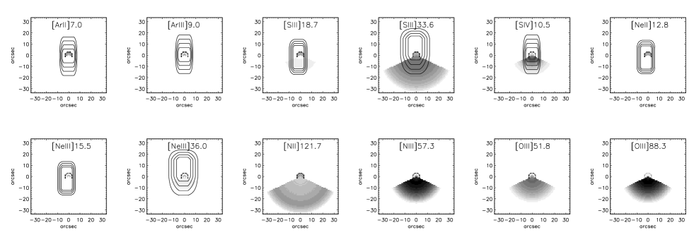
Figure 1: Emission lines maps of the best model, in grey linear scale. The two componets are presented with angular size related to their corresponding covering factors. Contours for the ISO SWS beam profile are superposed, for transmissions of 20, 40, 60, 80 % of the flux. In the four latest maps, the LWS aperture size is of order of the images, and not shown. Note that the SWS aperture is not always centered.

3.2 Atmosphere models

The ionizing photons distribution is taken from the recent CoStar atmosphere models, which include non-LTE effects, line blanketing, and stellar winds (Schaerer & de Koter 1997). The CoStar atmospheres have been compared to earlier predictions (Kurucz models and plane parallel non-LTE atmosphere models). Their implications on nebular studies have also been discussed by Stasińska & Schaerer (1997) and Schaerer & Stasińska (1999).

The predicted ionizing fluxes have been “tested” by the following indirect means:

• the CoStar SEDs reproduce well the ionic Ne⁺⁺/O⁺⁺ abundance ratios in Galactic H ii regions observed from optical and IR data, thereby solving the so-called [Ne iii] problem (Stasińska & Schaerer 1997). This supports the important increase of the ionizing spectra predicted at energies $\ga$ 35–40 eV.

• the observed increase of the ratio of the He⁰ over H⁰ ionizing photons between stellar effective temperatures of $\sim$ 30000 and 40000 K is well reproduced (Schaerer 2000). This quantity, sensitive to the ionizing flux above 13.6 and 24.6 eV, is constrained by optical He i recombination line measurements in the sample of Kennicutt et al. (2000) of H ii regions with known stellar content.

• Tailored photoionization models for two nebulae with exciting stars of spectral types O3-O4 and O7 respectively have been constructed by Oey et al. (2000) using CoStar spectra. While overall the spectra are found to yield a good agreement with the observed nebular line ratios for all objects (confirming also the first point), there is some indication of an overprediction of the spectrum above $\sim$ 35–40 eV for the early-type object (DEM L323). We note, however, that for DEM L243, this discrepancy is not found if a cooler spectrum is adopted (approximately model B2 instead of C2 preferred by Oey et al.), as would be expected for the region whose ionizing flux is likely dominated by the O7If supergiant instead of the O7V((f)) dwarf (cf. Vacca et al. 1996).

For the range of stellar temperatures of interest here ($T_{\rm eff}\sim$ 28–34 kK; cf. below) only 1 and 2 are directly applicable here. Indeed, at these relatively cool effective temperatures the uncertainties in the CoStar models are expected to be the largest, as stressed by Schaerer & de Koter (1997). Although the constraints on the atmosphere models are still rather limited, we conclude from the above comparisons that the adopted model atmospheres should provide a reasonable description of the ionizing fluxes. Comparisons with other model atmospheres are discussed in Sect. 5.6.

From the 27 CoStar models available on the Web (Schaerer & de Koter 1997), a finer grid of spectral energy distributions was constructed. For any effective temperature $T_{\mathrm{eff}}$ and luminosity $L$ in the range covered by the CoStar models, an interpolation is performed between the four nearest models of this grid, using the square inverse of the distance in the $\log T_{\rm eff}$–$\log L$ plane to determine the weights of the four CoStar models. The four CoStar models are first divided by the corresponding blackbody spectra, then averaged using the weights previously determined and the result is finally multiplied by the blackbody spectrum of the desired $T_{\mathrm{eff}}$ and $L$, avoiding the diktat of the most intense CoStar model.

3.3 Two-component model

In order to reproduce both r${}_{[{O\textsc{iii}}]}$ and the radio flux densities which imply a higher density (see Sect. 2.2), a two-component model is used to describe G29.96. The two components differ by their densities; the lower and higher density components are named component 1 and 2 respectively.

The present model consists of a simple linear combination of two independent runs of NEBU in a spherical case and under isobar approximation. Both components are assumed to be radiation bounded. The gas is supposed to be homogeneously distributed in each component, with an inner radius to reproduce an empty cavity. The coefficient applied to each component to obtain the fluxes of the emission lines is the covering factor, i.e. the angular size over 4 $\pi$ of each component as seen by the central source. The sum of the two covering factors is set to one, i.e. we do not consider that photons could escape from the H ii region. In this model, there is no diffuse radiation exchanged between component 1 and 2, and no effects of shielding of one component by the other is taken into account as: component 2 has a very small geometrical thickness compared to component 1, and component 1 is very optically thin at radio wavelengths. A two-component model must be seen as an approximation, describing the two first moments of a certainly more complicated gas distribution.

The most important effect of this 2-density medium is in the localization of the lines emission, which depends on their critical densities. For example, the [O III] and [N III] lines are emitted only by the lower density part of G29.96, because these lines are collisionally de-excited in the densest region (see Paper II for the critical densities of all the lines).

3.4 The ISO beam profiles

Component 1 of the nebula will have a larger geometric extension than component 2 due to its lower density. The beam sizes of the ISO instruments, which vary from 14-33 arcsec for the SWS to $\sim$ 80 arcsec for the LWS, have a drastic impact when comparing/dividing different emission lines. The beam profiles, from Garcia-Lario (1999), are used to apply a correction to the predicted line fluxes. For each component and line, an intensity map is generated by projection of the line emissivity on a sky plane. An “ISO” mask is then applied, according to the detector beam corresponding to the line wavelength.

Fig. 1 shows the intensity maps obtained for our best model (presented in Sect. 4) for 8 atomic lines. Contours of the corresponding ISO SWS apertures are superimposed on the image. For the four last images corresponding to lines observed by LWS, the aperture size is larger than the image. For most of the lines, only the core is visible with the adopted linear intensity scale. Note that, despite the absence of visible extended emission, for most of the lines the contribution of the extended part is about that of the core. The low density extended component is clearly seen for the low critical density lines for which the contribution of the core is very low (the [N II], [N III], [O III] and [S III] lines). The effect of neglecting the finite aperture size is clearly illustrated. Note also that the profile of the SWS aperture, as described by Garcia-Lario (1999), is not symmetrical. We did not attempt to exactly adjust the orientation of these profiles to the observations of G29.96, as the effect of the asymmetry in the profiles is negligible compared to the effect of departure from spherical symmetry of the object itself.

4 Results

4.1 Convergence procedure

Table 1 lists the parameters of the best two-component model and the observable used to constrain each parameter. In the following we describe the convergence procedure of this model.

The [O iii] lines are collisionaly de-excited in component 2 and trace mainly component 1, while the other density diagnostic lines are emitted by both components of the nebula. Therefore the [O iii] 51.8/ 88.3$\mu$m ratio is used to constrain the density of component 1. The density of component 2 is constrained by the 6 cm radio flux density. The ratio of the two covering factors is determined by fitting the Br$\alpha$ line flux, the sum beeing fixed to 1.

Fig. 2 shows the four available [Xⁱ]/[Xⁱ⁺¹] line ratios (divided by the corresponding observed values) versus the effective temperature of the ionizing star, namely [Ar ii] 6.98$\mu$m/[Ar iii] 8.98$\mu$m, [S iii] 18.7$\mu$m/[S iv] 10.5$\mu$m, [Ne ii] 12.8$\mu$m/[Ne iii] 15.5$\mu$m and [N ii] 121.7$\mu$m/[N iii] 57.3$\mu$m. The number of ionizing photons is kept constant by adjusting the number of ionizing stars with fixed luminosity, while the effective temperature is varied. The models used for this plot are all 2-component models. In the range of $T_{\rm eff}$ considered here (27 to 35 kK) the sensitivity of those ratios to the effective temperature is very high (see also Stasińska & Schaerer 1997, and Paper II). Within a range of $\sim$ 2500 K, the four ratios provide the same constraint on the effective temperature. However, the [Ar ii] 6.98$\mu$m/[Ar iii] 8.98$\mu$m ratio gives a higher effective temperature than the three other diagnostics (see Sect. 5.6). We will therefore use the [N ii] 121.7$\mu$m/[N iii] 57.3$\mu$m ratio to determine the effective temperature, as it is: 1) independent of the ISO beam size since both lines were observed with LWS, and 2) emitted only by component 1, since it is collisionaly de-excited in component 2. An effective temperature of $\sim 30^{+2}_{-1}$ kK is then derived.

Figure 2: Variation of the four [Xⁱ]/[Xⁱ⁺¹] ratios with the effective temperature. The ratios correspond to: Ar (solid) , S (dot), Ne (dashed) and N (dot-dashed) and have been divided by their corresponding observed values.

Table 1: Parameters of the best model and derived gas properties. For some parameters, the observable used for the main constraint is given.

Parameters common for both components
Effective temp (kK)	29.7	from [N ii] 121.7$\mu$m/[N iii] 57.3$\mu$m
Luminosity in log(L/L⊙)	5.861	from borderline in CoStar models grid (see Sect. 5.8)
Number of stars	1.5	from 2 cm flux density (see Sect. 5.5)
Inner radius ($10^{17}$ cm)	3.	from imaging
Dust/gas ratio	$10^{-5}$	from ISO continuum emission
[He]/[H] (in numbers)	0.1
[C]/[H]	1.00$\times 10^{-4}$
[N]/[H]	1.97$\times 10^{-4}$	from [N ii] 121.8$\mu$m + [N iii] 57.3$\mu$m
[O]/[H]	4.55$\times 10^{-4}$	from [O iii] 51.8 + 88.3$\mu$m
[Ne]/[H]	1.70$\times 10^{-4}$	from [Ne ii] 12.8$\mu$m + [Ne iii] 15.5$\mu$m
[S]/[H]	2.25$\times 10^{-5}$	from [S iii] 18.7$\mu$m + [S iv] 10.5$\mu$m
[Ar]/[H]	5.00$\times 10^{-6}$	from [Ar ii] 6.98$\mu$m + [Ar iii] 9.0$\mu$m
Parameters for:	Component 1	Component 2
Inner nH (cm-3)	640. from r${}_{[{O\textsc{iii}}]}$	52000. from 6 cm flux density
Covering factor	36 %      and	64 % from Br$\alpha$
Filling factor	1.00	1.00
Properties for:	Component 1	Component 2
Mean ne (cm-3)	680.	57000.
Constant pressure (cgs)	9.7$\times 10^{-10}$	1.1$\times 10^{-7}$
Thickness (1017 cm)	27.2	0.15
Mass (M⊙)	29.	0.73
Mean T${}_{H\textsc{ii}}$ (K)	5520	7230
inner U	8.8$\times 10^{-1}$	5.7$\times 10^{-3}$

¹ This luminosity multiplied by the number of stars leads to $1.8\times 10^{49}$ ionizing photons (N_Lyc).

The total luminosity is the product of the CoStar model luminosity by the number of stars, and the number of ionizing photons is adjusted to reproduce the radio flux density at 2 cm. A range of stars with different spectral types is presently not considered. With the available CoStar models, there is an upper limit for the star luminosity beyond which no more models are available and which corresponds to the post main sequence or Wolf-Rayet star regime. The degeneracy of the CoStar model luminosity by the number of stars is discussed in Sect. 5.5.

Once the above set of parameters is fixed, the abundance of each species is derived by fitting their lines fluxes. As most of the parameters have feedback effects, an iterative process must be applied.

To summarize, we have 17 free parameters (listed in Table 1), namely: effective temperature and luminosity of one star, number of stars, densities of both components, ratio of the covering factors, inner radius of the empty cavity, dust to gas ratio, filling factors of both components, and 7 abundances. On the other hand, we have 16 observables plus the morphology of the source as given by the radio maps.

Some parameters (the inner radius, the dust/gas ratio, the filling factors) cannot be precisely constrained and are set to a reasonable value. Change in their values are discussed in Sect. 5. The abundance of helium and carbon does not have any effect on the results of the model, if remaining within reasonable values.

We finally stay with 11 free parameters to be constrained by 17 observables. In other words, there are 6 observables that are not used to build the model and are therefore entirely predicted, namely: the three [Xⁱ]/[Xⁱ⁺¹] ratios for Ne, Ar and S, the two [S iii] 33.6$\mu$m and [Ne iii] 36.0$\mu$m line fluxes (not used because of their large calibration error, see Paper I and Paper II), and the 21 cm continuum flux density.

4.2 Results and predictions

Table 2 lists the observations of the infrared emission lines and the radio continuum flux densities together with the results of the best model. The contributions of the two density components are given separately. Most of the predicted lines fluxes and radio flux densities agree with the observations to within the uncertainties of the measurements. The few predictions which are off by a larger factor are the results of well understood factors which will be explained hereafter.

The three [Xⁱ]/[Xⁱ⁺¹] ratios not used to determine the effective temperature agree within $\sim$ 1 kK with the [N ii] 121.7$\mu$m/[N iii] 57.3$\mu$m ratio (see Fig. 2). The [S IV] 10.5$\mu$m line falls in the absorption feature due to silicate. This has been taken into account when using the attenuation law described in Paper II and the model prediction is in very good agreement with the observation. For [Ne III] 15.5$\mu$m, we can suspect an overprediction of the line flux due to the used of the CoStar models, as discussed by Oey et al. (2000) and in Sect. 3.2 (see also Sect. 5.6).

Note that the predicted 21 cm flux density is lower than the value observed by Kim & Koo (2001), who reported complex extended radio emission toward G29.96. Part of this diffuse emission could be due to gas ionized by members of the stellar cluster other than the main ionizing star of G29.96. This low excitation gas is not taken into account in the present model.

Table 2: Observations and model predictions. The model fluxes for each component are already multiplied by the ISO SWS aperture correction factor (given in parenthesis for component 1, component 2 being small enough to be entirely seen by both ISO spectrometers) and by the covering factor corresponding of each component.

Line	Line fluxes (10-18 W/cm2)					Model/Observation
	Observations1	Model	Component 1		Component 2
H i 4.05$\mu$m	11.4 $\pm$0.4	11.4	.900	(.16)	10.5	1.00
[Ar ii] 6.98$\mu$m	27.1 $\pm$3.0	36.3	1.34	(.08)	34.9	1.34
[Ar iii] 8.98$\mu$m	20.5 $\pm$1.4	13.1	2.21	(.23)	10.9	0.64
[S iii] 18.7$\mu$m	64.7 $\pm$1.2	55.5	25.0	(.21)	30.4	0.86
[S iii] 33.6$\mu$m	44.32 $\pm$3.0	23.8	20.8	(.18)	2.95	0.542
[S iv] 10.5$\mu$m	7.90 $\pm$0.8	8.95	7.70	(.51)	1.25	1.13
[Ne ii] 12.8$\mu$m	127.5 $\pm$9.0	97.8	6.08	(.13)	91.7	0.77
[Ne iii] 15.5$\mu$m	34.0 $\pm$1.3	42.5	15.9	(.43)	26.6	1.25
[Ne iii] 36.0$\mu$m	3.282 $\pm$1.0	2.37	1.18	(.38)	1.18	0.722
[N ii] 121.8$\mu$m	4.66 $\pm$0.2	4.65	4.50		.150	1.00
[N iii] 57.3$\mu$m	23.0 $\pm$0.7	23.1	22.6		.540	1.00
[O iii] 51.8$\mu$m	47.4 $\pm$0.2	47.6	45.6		2.08	1.00
[O iii] 88.3$\mu$m	19.7 $\pm$0.4	19.6	19.4		.210	0.99
Wavelength (freq.)	Continuum flux density (Jy)
2 cm (15 GHz)	3.90 $\pm$0.5	3.90	1.34		2.57	1.00
6 cm (5 GHz)	3.40 $\pm$0.2	3.38	1.53		1.84	0.99
21 cm (1.4 GHz)	2.60 $\pm$0.2	1.88	1.60		.282	0.72

¹ The line fluxes (from Paper I) are corrected for the interstellar extinction using A${}_{K}=1.6$ and the law described in Paper II.

² Line measured with the SWS band 4 detector, see Paper I.

5 Discussion

The detailed photoionization model of G29.96 reproduces with good accuracy most of the atomic fine-structure line fluxes and radio flux densities. It allows one to derive the elemental abundances in the gas phase and the properties of the ionizing star(s). In the following, we will investigate how some of the less constrained parameters influence the results and discuss the reliability of the derived abundances.

5.1 Effect of the uncertainties of the observed line fluxes on the model parameters

The observed line fluxes are known with 10 to 20 % accuracy (Paper I). The effect of these uncertainties on the model are not always linear. For example, changing r${}_{[{O\textsc{iii}}]}$ by $\pm 20$ % changes the electron density of component 1 by ${}^{+34}_{-25}$ %. On the other hand, as the stellar effective temperature diagnostics are extremely sensitive (as shown in Fig. 2), any change by $\pm 20$ % in any of these diagnostic line fluxes will have virtually no effect on the determination of the stellar temperature.

Concerning the number of ionizing photons, the product of the number of stars by the stellar luminosity is directly proportional to the 2 cm flux density.

One of the most critical parameters is the contribution of each component to the total line fluxes. Once the density of component 2 is determined from the 6 cm flux density, the ratio of the covering factors is derived by fitting the Br$\alpha$ line flux. However, this line is sensitive to attenuation and aperture size corrections. As given in Table 2, the nitrogen and oxygen lines are emitted mainly (96 to 99 %) by the diffuse component where only 10 % of the hydrogen lines emission is observed. Decreasing the observed line flux of Br$\alpha$ by 10 % increases the contribution of component 1 from 36 % to 48 % and the density of component 2 from 5.2$\times 10^{4}$ to 9.0$\times 10^{4}$ cm^-3. The abundances of N, O, Ne, S, and Ar change by $-25,-30,+10,0,$ and $+20$ % respectively.

5.2 Filling factor and components geometry

The filling factor allows one to artificially increase the geometrical thickness of the ionized gas. The geometry affects both the low and high ionized species if the thickness of the nebula is of the order of its radius.

As component 1 represents the diffuse gas, a filling factor of 1.0 seems appropriate (the predicted extension of the gas is 35”, i.e. comparable to the size of the observed surrounding molecular gas). Lowering this filling factor to 0.5 has an effect on the lines mainly produced by component 1, i.e. [N II] 121.8$\mu$m, [N III] 57.3$\mu$m, [O III] 51.8, 88.3$\mu$m, [S iii] 33.6$\mu$m, and [S IV] 10.5$\mu$m. The ratio r${}_{[{O\textsc{iii}}]}$ remains the same while the [N II] 121.8$\mu$m/ [N III] 57.3$\mu$m ratio increases by about 15 %. A small increase of the effective temperature from 29.7 to 30.1 kK is enough to recover the observed ratio. After the whole convergence process is performed, an increase of the N and O abundances of about 15 % is found. Furthermore, as the geometrical thickness of component 1 increases up to 45”, the effects of the finite size of the ISO SWS beam are amplified (the [S IV] 10.5$\mu$m line significantly decreases). No value lower than 0.5, implying greater geometrical extension, would be acceptable.

For component 2, changing the filling factor from 1.0 to 0.5 increases the thickness by a factor of about two. No obvious effect is found on the line fluxes, but the radio flux densities are affected because the self absorption is decreasing with the filling factor. The predicted 6 cm value is then higher than the observed value by 8 %, and we have to change the hydrogen inner density of component 2 from 5.2 to 9.2$\times 10^{4}$ cm^-3 to recover it. The geometrical thickness of component 2 finally decreases from 1.5 to 1.0$\times 10^{16}$ cm, the changes due to the filling factor being approximatively compensated by the increase of density imposed by the 6 cm flux density constraint. However, the line fluxes and the element abundances do not change significantly.

Decreasing further the filling factor of component 2 to a value of 0.1 leads to a different behavior. The hydrogen density needs to be increased to 5.5$\times 10^{5}$ cm^-3 in order to recover the optical thicknesses of the radio continuum at various frequencies. Such a high density implies a collisional de-excitation of some lines in component 2 (see Paper II for the critical densities of all the lines). Finally, the abundances are greater than those given in Table 2 by 4, 7, 77, 83, 111 % for N, O, Ne, S, Ar, respectively. Oxygen and nitrogen are not very affected as these lines are emitted in component 1. The geometrical thickness of component 2 becomes 1.6$\times 10^{15}$ cm. We could interpret this model as a distribution of very dense, small clumps embedded in the low density medium.

In summary, modifying the filling factor leads to a change of the geometry of the ionized gas. The main effect is on the self-absorption of the radio free-free emission; changing the filling factor is the same as changing the optical depth at the different radio frequencies, in other words, changing the proportion of the gas seen tangentially with respect to the amount of gas seen radially.

Afflerbach et al. (1994) derived a filling factor between 0.03 and 0.4 combining the emission measure obtained from the continuum flux density with the local density obtained from the line-to-continuum ratio. They found high values for the density (some 10⁴cm^-3) and they considered the gas as included in a sphere: “assuming that the line-of-sight depth is equal to the angular diameter from the continuum images”. In our case, the dense gas is located in a shell (in which the filling factor is $\sim$ 1.0) with a thickness 1/20 of its radius, leading to a total filling factor for the sphere of 0.13, compatible with the value obtained by Afflerbach et al. (1994). In the model presented in this paper, the gas is distributed in a shell, at fixed radius from the ionizing source. A more complex model could be constructed with a distribution of clouds at various radii, but the new free parameters introduced in such a model could not be constrained by any available observable.

5.3 Role of the inner radius

We fixed the inner radius of the H ii region to $3\times 10^{17}$ cm, corresponding to 3”, about the radio core size (e.g., Fey et al. 1995). This is also virtually the outer radius of the dense component, as the geometrical thickness is 1/20 times the inner radius. Lowering the value to e.g. $10^{17}$ cm will require to decrease the density of component 2 to $2.2\times 10^{4}$ cm^-3 in order to recover the radio flux densities break between 2 and 6 cm. The geometrical thickness of component 2 is now $\sim 2\times 10^{17}$ cm, still compatible with imaging observations. Oxygen and nitrogen abundances must be decreased by 10 %. As the density of component 2 decreases, some lines previously de-excited by collisions in component 2 are now emitted: [Ne iii] 15.5$\mu$m and [S iv] 10.5$\mu$m are predicted to be 3 and 5 times higher than the observed values.

Increasing the inner radius for component 2 will lead to an increase of the density of this component to recover the radio break. As the geometrical thickness will then decrease to less than one percent of the radius (it was 5 % for the adopted model, see Table 1), the self absorption at 6 cm does not increase anymore. This is mainly due to the spherical geometry we used for the model. A more complicated geometry than such a thin shell could lead to more self-absorption. We then relax the constraint of the 6 cm flux density and perform a model where the 6 cm predicted flux density can be higher than the observation by some 10 %. With a density of $8\times 10^{4}$ cm^-3 for component 2, and an increase or N, O, Ne, S, and Ar abundances of 12, 12, 24, 30, and 10 % respectively, the result is close to the adopted model.

5.4 Role of dust

The effect of adding dust in the H ii region is to increase the absorption of ionizing photons and to change the shape of the “apparent” ionizing spectrum. We compared the emitted spectra of the dust to the observed infrared continuum, at wavelengths lower than 20 $\mu$m. At longer wavelengths, the emission is dominated by cold dust from the PDR and the outer H i region, which is not modeled by the photoionization code. We check that, whatever the dust type used (i.e. ”astronomical” silicates, olivines, amorphous carbon or graphite), the modeled emission does not exceed the observational data for any concentration of dust lower than $5\times 10^{-4}$ (in mass, relative to hydrogen). This represents an upper limit of the amount of dust, as part of the 5-20 $\mu$m emission can be due to high temperature PAH’s present in the PDR and behind. With this amount of dust, the models have to be adjust by changing the number of stars from 1.5 to 1.6 and the stellar effective temperature from 29.7 to 29.4 kK, without changes in the abundances. In this “maximum” dust model, 8% of the incoming energy is absorbed by dust in the H ii region, compared to 11% by ions. The relatively small amount of dust derived by our modeling is in agreement with the recent results of Aannestad & Emery (2001) who found that dust in the ionized region of S 125 is severely depleted. A more detailed study of the dust emission observed in G29.96, including the H i region, is postponed to a future paper.

5.5 Number of stars versus luminosity and age

Figure 3: HR diagram showing the locations of the available CoStar models (crosses) and the four models discussed in text (filled diamonds with corresponding number of stars). The dotted lines show solar metalicity isochrones for ages 0, 1.6, 2.8, 3.5 and 4.0 Myr from left to right, from the tracks of Meynet et al. (1994).

The number of ionizing photons is constrained by the 2 cm radio flux density. It is a degenerated parameter since it is the product of the number of stars by the number of ionizing photons produced by one star. This degeneracy can be explored by changing the luminosity of the individual stars and by adjusting the corresponding value of the number of stars.

If one changes the luminosity of the individual stars, the effective temperature of each star must be changed in order to recover the [N ii] 121.7$\mu$m/[N iii] 57.3$\mu$m ratio. All the fluxes are then reproduced as in the adopted model presented in Table 2 within a few percent. Fig. 3 shows in an HR diagram the locations of the available CoStar models (crosses) and the four models retained and discussed here (filled diamonds). The number of stars needed to reproduce the 2 cm flux density is given for each model. Although the range in effective temperature seems small (from 30 to 35 kK), it is large if one considers the strong constraint from the [N ii] 121.7$\mu$m/[N iii] 57.3$\mu$m ratio (see Fig. 2). Along the track between the four models with 1.5, 3.3, 8.6 and 19 stars, the stellar age varies approximatively from 2.8, 3.5, 4.0 to 1.6x$10^{6}$ yr. Whatever the exact number of stars involved in the ionization of G29.96, we see that these stars occupy a rather small range in effective temperature (30 to 35 kK) and age (1.6 to 4 Myr). The obtained ages are quite old compared to “classical” expectations for UCHII regions.

We cannot find a satisfying model corresponding to one single star, as the luminosity will then overstep the CoStar models grid and enter the post main sequence and/or Wolf Rayet (see Fig. 3). Once the temperature is derived from the diagnostic lines ratio [N ii] 121.7$\mu$m/[N iii] 57.3$\mu$m, we used the most luminous star available and multiply its flux by a factor 1.5 to reproduce the radio flux . As we know from NIR observations (see Sect. 2.4) that only one star is the primary source of ionization, we think our model with 1.5 star is better. We can interpret the value of 1.5 star as a consequence of mixing one main ionizing star with one or more lower luminous stars.

5.6 Dependence on atmosphere models

The derived parameters of the ionizing source depend on the adopted atmosphere models. Given the limited amount of constraints available on the ionizing fluxes (cf. Sect. 3.2) and the potential uncertainties of the CoStar models especially for cool stars with weak winds (Schaerer & de Koter 1997), we have also tested other non-LTE model atmospheres. A full description is given in Morisset et al. (2002). Here we summarize the main effects.

We have used the recent line blanketed models of Pauldrach et al. (2001) and test calculations for O stars based on the comoving frame code CMFGEN of Hillier & Miller (1998) which both include stellar winds. Spectra from the fully blanketed plane parallel non-LTE TLUSTY models of Hubeny & Lanz (1995) were also kindly made available to us by Thierry Lanz. The comparison of the predicted IR fine-structure line ratios with observations from the sample of Paper I & II shows that a consistent fit of all four ratios ([N iii]/[N ii], [Ar iii]/[Ar ii], [S iv]/[S iii], [Ne iii]/[Ne ii]) within a factor of two is only obtained with the CoStar models. The scatter in the effective temperature determined with the CoStar models is due to the [Ar iii]/[Ar ii] ratio, which have a similar ionization potential than [N iii] (29.6 and 27.6 eV respectively), showing a potential problem in either the observed line fluxes, the attenuation correction process, or in the atomic data. The other three excitation ratio, tracing ionizing photons between 27.6 and 40.1 eV, are in a very good agreement. as also seen for G29.96.

Using the extreme excitation ratio of [N iii]/[N ii] and [Ne iii]/[Ne ii], we estimate effective temperatures of $\sim$ 32–35, 33–38 and 34–38 kK, using the models CMFGEN of Hillier & Miller (1998), TLUSTY of Hubeny & Lanz (1995), and WM-Basic of Pauldrach et al. (2001) respectively, while the same ratio leads to lower and less scattered effective temperatures (29.5–30.5 kK) using the CoStar models (see fig. 2).

5.7 Other constraints and comparison with earlier studies of the exciting star

Various estimates of the properties of the dominant ionizing star of G29.96-0.02 have been obtained from the following observations/methods:

1. the bolometric luminosity $L$, estimated from IR or multi-wavelength observations

2. the photon flux in the Lyman continuum $N_{\rm Lyc}$ assuming a single star,

3. the ratio $N_{\rm Lyc}/L$ for a stellar cluster,

4. IR line ratios through nebular modeling,

5. the He⁺ abundance derived from radio recombination lines,

6. near-IR photometry, and

7. K-band spectral classification of the central source.

The estimated spectral types quoted in the literature reach from O3 to O9.5 (e.g., Lacy et al. 1982; Doherty et al. 1994; Simpson et al. 1995; Afflerbach et al. 1997; Watson et al. 1997; Kaper et al. 2002). However, these estimates are partly based on incompatible hypothesis such as different assumptions on the source distance and different spectral type vs. $T_{\mathrm{eff}}$ calibrations. Furthermore only unevolved zero age main sequence (ZAMS) stars were considered in most cases, in conflict with recent evidence (Afflerbach et al. 1997, this paper). For these reasons we here briefly rediscuss these estimates using also up-to-date stellar models and homogeneous assumptions. In particular all observational constraints are scaled to a distance of 6 kpc (cf. Sect. 2.3). As $T_{\mathrm{eff}}$ is the physically most important parameter – independently of the exact spectral-type vs. $T_{\mathrm{eff}}$ relation – we essentially derive the constraint on this parameter.

1) The total bolometric luminosity of G29.96 obtained from the 12-100 $\mu$m IRAS flux and its overall SED in an arcminute sized region is $\log L/L_{\odot}$ $\sim$ 5.90 (Paper I, Afflerbach et al. 1997). Likely the major fraction of it is due to the main ionizing source (cf. Afflerbach et al. 1997, and below). Using the calibrations of Schmidt-Kaler (1982) yields the following $T_{\mathrm{eff}}$: $\sim$ 44 kK (for luminosity class V), 41 kK (LC III), 37 kK (LC I). From Vacca et al. (1996) one obtains: $\sim$ 48 kK (LC V), 45 kK (LCIII), 36 kK (LC I). A very wide range of $T_{\mathrm{eff}}$ ($\ga$ 20 kK to $\la$ 50 kK) is allowed for main sequence stars with the given luminosity, as shown in Fig. 3. These $T_{\mathrm{eff}}$ represent upper limits as other stars contribute to the total bolometric (cf. below).

2) The ionizing photon flux derived for G29.96 from radio emission is $\log(N_{\rm Lyc})\sim$ 49.–49.14 s^-1 (Fey et al. 1995; Kim & Koo 2001). A somewhat higher value of $\log(N_{\rm Lyc})\sim$ 49.29 was derived by Afflerbach et al. (1997) from the extinction corrected Brackett-$\gamma$ map. Based on the Vacca et al. (1996) calibrations this corresponds to $T_{\mathrm{eff}}$ $\sim$ 40–43 kK (LC V), 35–38 kK (LC III), and 30–32 kK (LC I). Similarly, the stellar models of Schaerer & de Koter (1997) (based on the tracks shown in Fig. 3) reproduce the observed $N_{\rm Lyc}$ for a temperature range between $\sim$ 30 and 46 kK, depending on the evolutionary state.

3) Given the obvious importance of small number statistics for the number of massive stars observed in the cluster associated with G29.96 (see Afflerbach et al. 1997; Pratap et al. 1999) standard evolutionary synthesis models cannot be used for comparisons of $N_{\rm Lyc}/L$ (Cerviño et al. 2000). However, an analysis of the resolved stellar content provides further insight. As discussed by Afflerbach et al. (1997); Pratap et al. (1999) we have taken the objects with $H-K\geq 1.$ as cluster members. Assuming a mean extinction $A_{H}=3.6$ (Afflerbach et al. 1997) and using the synthetic photometry of Lejeune & Schaerer (2001) we have determined from the H-band magnitude $m_{H}$ the luminosity of the individual stars assuming all members to be on the same isochrone with ages between $\sim$ 0 and 4 Myr. From this we derive the fraction of $L$ provided by the ionizing star, which is found to be $\sim$ 70–50 % for ages 0–4 Myr. A somewhat smaller fraction (70–30 %) is found using $m_{K}$ (and $A_{K}=2.14$). This quantitative estimate confirms the expectations of Afflerbach et al. (1997) of a contribution of at least 50 % from the ionizing star to $L$. Correcting for $\sim$ 50 % of $L$ due other cluster members and assuming that one star dominates the ionization, we obtain a revised $N_{\rm Lyc}/L$ of the ionizing star which should be comparable to predictions for single stars. The comparison with the stellar models used earlier yields $T_{\mathrm{eff}}$ between $\sim$ 31 and 38 kK.

4) Simpson et al. (1995) and Afflerbach et al. (1997) used line measurements from KAO and photoionization models including plane parallel LTE Kurucz model atmospheres. Their analysis (method 4) yields $T_{\rm eff}=$ 35.7 and 37.5 kK respectively, rather similar to our values derived with different atmosphere models, but larger than the value obtained with the CoStar atmosphere models. The main difference with their result likely originates from the use of more sophisticated model atmospheres.

5) The He⁺/He ionization fractions derived for the best model presented in Table 2 are 50 % (35 %) for Component 1 (2) respectively, slightly lower than the values obtained by Kim & Koo (2001): 68 to 76 %. Using hottest stars with CMFGEN at 33 kK and WM-Basic at 36 kK atmosphere models, we found He⁺/He to be 60 % (48%) and 77 % (68 %) respectively, in better agreement with the value obtained by Kim & Koo (2001) (but see the discussion on the Xⁱ⁺¹/Xⁱ ratios for Ar, Ne, N and S in Sect. 5.6).

6) From photometric observations and constraints on the total luminosity of G29.96 (Afflerbach et al. 1997) derive an allowed temperature range for the ionizing star of $T_{\mathrm{eff}}$ $\sim$ 28–37 (23–43) kK at for 1 (3) $\sigma$ uncertainties valid for source distances between approx. 5–9 kpc. Our above analysis of the cluster photometric data, taking the the contribution of all individual objects to $L$ into account, yields consistency only for ages $\sim$ 3–4 Myr. Despite this, the permitted $T_{\mathrm{eff}}$ range based the H or K band data remains fairly large, and essentially identical to the above values.

7) Watson & Hanson (1997) obtained the first K-band spectrum of the ionizing star of G29.96, whose spectral type was found between O5 and O8 (luminosity class undetermined; cf. Watson & Hanson 1997), based on the presence of He ii absorption, and C iv and N iii emission lines. They note, however, that a O7 or O8 spectral type would require some enhancement of the C iv and N iii features – attributed to a higher metallicity – compared to “normal” objects of these types. While the recent VLT spectrum presented in the preliminary work of Kaper et al. (2002) appears to be consistent with the data of Watson & Hanson (1997), the former authors deduce a spectral type as early as O3 based on the presence of the C iv and N iii emission lines. From this it appears that a more detailed analysis of the data of Kaper et al. (2002) should be awaited before more firm conclusions on the spectral type of G29.96 can be drawn.

In any case, given the unknown luminosity class the following temperature ranges are obtained for O5–O8 (O3): $\sim$ 38.5–46 kK (51 kK) for LC V, intermediate values fo LC III, and $\sim$ 36–45 kK (50 kK) for LC Ia using the Vacca et al. (1996) compilation based on analysis using pure H-He atmosphere models. Recent fully line blanketed non-LTE calculations including stellar winds show, however, that – as already suspected earlier – the $T_{\mathrm{eff}}$ scale of O stars must be cooler (e.g., Fullerton et al. 2000; Martins et al. 2002).

The models of Martins et al. (2002) yield a reduction of $T_{\mathrm{eff}}$ by 4 to 1.5 kK for O3–O9.5 dwarfs compared to the Vacca et al. (1996) scale, and larger reductions are expected for giants and supergiants. Taking these effects into account we estimate for O5–O8 types $T_{\mathrm{eff}}$ $\sim$ 36–43 kK for LC V and $\sim$ 33–40 kK for LC Ia.

Combining the available data it appears that the preliminary spectral classification by Kaper et al. (2002) is the only information which is incompatible with most other constraints (points 3-6, possibly also 1 and 2). Good consistency is obtained, however, from the intersection of the above constraints 1) to 6), yielding an allowed $T_{\mathrm{eff}}$ between $\sim$ 31 and 37 kK, overlapping with the spectral type derived by Watson & Hanson (1997). We thus conclude that overall the parameters derived from our photoionization modeling are compatible with all the available observational data.

Table 3: Abundances determined by previous authors and in the present work.

Element	Herter et al. (1981)	Simpson et al. (1995)		Afflerbach et al. (1997)		Paper II		This work	Solar2
	G29.96	G29.96	4.5 kpc1	G29.96	4.5 kpc1	G29.96	4.5 kpc1
N/H (10-4)	–	2.3	1.8	1.8	1.2	1.9	–	2.0	0.8
O/H (10-4)	–	8.5	6.6	5.6	7.3	5.1	–	4.6	6.8
Ne/H (10-4)	2.7	2.6	1.8	–	–	2.5	2.2	1.7	1.2
S/H (10-5)	3.2	1.9	1.6	2.2	1.8	0.8	–	2.2	2.1
Ar/H (10-6)	23.	–	–	–	–	4.8	5.0	5.0	2.5
N/O	–	0.27	0.27	0.32	0.17	0.37	0.33	0.43	0.12
Ne/S	8.4	13.	11.	–	–	36.	–	7.5	5.7

¹ Values obtained applying the gradients from the corresponding authors at the galactocentric distance of G29.96

² from Grevesse & Sauval (1998).

5.8 Implications of the advanced age of G29.96

However, an age of $\simeq 3\times 10^{6}$ years for the star is very high compared to the expected dynamical lifetime of UCHII regions ($5\times 10^{5}$ years, see e.g., Wood & Churchwell 1989a, based on the number of UCHII regions in the Galaxy and their expected lifetime). Two main models have been developed to explain the cometary morphology which is common for UCHII regions. Models of stellar-wind bow shocks (see e.g., Mac Low et al. 1991), due to an O star moving supersonically through a molecular cloud, were first studied and applied to G29.96 (Wood & Churchwell 1991; van Buren & Mac Low 1992; Lumsden & Hoare 1996). Champagne flow models (see e.g., Yorke et al. 1983), resulting from the expansion of an H ii region into a molecular cloud exhibiting a density gradient, are also able to reproduce the cometary morphology. These models were applied more recently to G29.96 (Fey et al. 1995; Lumsden & Hoare 1996, PMB99) and were found to give results more consistent with the radio observations.

It is important to note that assuming a reasonable projected proper motion of 1 km/s, the star should have moved away from its birth place by about 3 pc (1.75 arcmin) in $\sim 3\times 10^{6}$ years. This rules out the Champagne flow model as a complete description of G29.96 and strongly favors the random meeting of an older star with an interstellar cloud. The ionizing star may also have left its birthplace, irradiating molecular gas further out which could still be part of the larger parental cloud from which it was formed.

5.9 Reliability of the abundances determination

The determination of the elemental abundances from the infrared fine-structure lines depends on many physical parameters, such as the filling factor, which are poorly constrained. Nevertheless,we can assert that there are two groups of elements. On one hand, oxygen and nitrogen, whose lines, all observed by the LWS spectrometer, are mostly emitted by the extended component 1, due to their low critical densities. Uncertainties in the attenuation correction and then in the Br$\alpha$ line flux by, e.g., 10 % leads to an uncertainty on the N and O abundances of 25 to 30 % (see Sect. 5.1).

The elements neon, argon and sulfur group, whose lines are observed by the SWS spectrometer (as the H i lines) with all the subsequent aperture corrections, are emitted by both components. The presence of high density clumps (filling factor of 0.1 – see Sect. 5.2) in the core will lead to abundances two times higher than what we determined in the presented model for the Ne, Ar, S group.

Whatever the uncertainties could be on the filling factor, the geometry of the source, the attenuation or the actual value of the radio emission, the determination of the abundance ratios in each group are robust: the N/O ratio on one hand, and the Ne/Ar, Ne/S and Ar/S ratios on the other.

Table 3 compares the abundances determined here and by Herter et al. (1981), Simpson et al. (1995), Afflerbach et al. (1997) and Paper II. The solar abundances from Grevesse & Sauval (1998) are also given. Afflerbach et al. (1997) used the Simpson et al. (1995) observations to modeled G29.96, but with a core/halo description. They both made semi-empirical models (using icf’s) and adopted an higher effective temperature ($\sim$ 36 kK, see discussion in Sect. 5.7). The method used in Paper II is semi-empirical, based on the same observed line fluxes as the present work. For those previous works, we give the values effectively determined for G29.96 and the values obtained using the abundance gradient law they found, applied at the position of G29.96: 4.5 kpc from the galactic center.

The set of abundances, exepted for oxygen, shows that G29.96 is overabundant compared to the solar values, in agreement with its inner position in the Galaxy. The abundances determined in the present work are compatible with the previous determination within a factor of 2, except with the Ar/H ratio from Herter et al. (1981) and S/H ratio from Paper II.

The determination of the sulfur abundance relative to hydrogen in Paper II is very different from what the previous authors and the present work found. From the results presented in Table 2 we see that the [S iii] 18.7$\mu$m and [S iv] 10.5$\mu$m lines on which the sulfur abundance is based in Paper II are mostly emitted by the extended component 1. The effect of the finite aperture size of the SWS instrument is crucial in this case. As there was no correction for this effect in Paper II, the sulfur emission and its abundance are underestimated.

6 Conclusion

This paper presents a detailed model of the compact Galactic H ii region G29.96 for which high quality data imagery and spectroscopy is available at both infrared and radio wavelengths, including recent ISO observations. The model, which is based on the photoionization code NEBU and state-of-the-art stellar atmosphere models, reproduces most of the observations, with the exception of a few points known to be less accurately measured. The radio and infrared data on G29.96 are best reproduced by a 2-density component model nebula, with a diffuse (n${}_{H}\sim 600$ cm^-3) extended (1 pc) halo surrounding a dense (n${}_{H}\sim 50000$ cm^-3) compact (0.1 pc) core.

Using CoStar stellar atmosphere models we derived an effective temperature of $\sim 30^{+2}_{-1}$ kK. Adopting more recent non-LTE line blanketed atmospheres with stellar winds, a somewhat higher $T_{\mathrm{eff}}$ $\sim$ 32–38 kK is found. This temperature range is compatible with all observational constraints. For $T_{\mathrm{eff}}$ $\sim$ 33-36 kK compatibility is also obtained with the K-band spectral type O5–O8 determined by (Watson & Hanson 1997) when recent downward revisions of the effective temperature scale of O stars (Martins et al. 2002) are taken into account.

We explored the effect of varying the different model parameters on the predictions. The main sources of uncertainty in determining the abundances are the fluxes of the hydrogen recombination lines and the geometry of the dense compact core.

The derived elemental abundances are in agreement with the lowest values found in previous studies. The most robust results are N/O and Ne/S which are 3.5 and 1.3 times the solar values, respectively.

From the reanalysis of the different available observational constraints (see Sect. 5.7) it is not surprising that several earlier studies reached apparently conflicting results on the spectral type or $T_{\mathrm{eff}}$ of the ionizing source of G29.96. This is mostly due to the following facts. First, proper photoionization models must account for the dependence of nebular lines on several parameters, including the ionization parameter, geometry etc. Second, consistent predictions from stellar models regarding ionizing fluxes, $T_{\mathrm{eff}}$ scales etc. should be used taking into account recent progress made with fully line blanketed non-LTE atmosphere models. Last, but not least, as the available K-band spectroscopy does not allow a determination of the luminosity class, allowance should be made for possible variations of the evolutionary state of ionizing sources in compact H ii regions. In view of these issues one may question whether mid-IR analysis of compact H ii regions yield intrinsically different estimates of $T_{\mathrm{eff}}$ compared to spectral types or other constraints as suggested by Hanson et al. (2002). Our detailed analysis of G29.96 indicates the opposite.

The age of the ionizing star required by our model is $\approx 3\times 10^{6}$ yr, much older than the expected lifetime of UCHII regions. This could indicate that G29.96 is not excited by a bona fide young massive star. Instead the ionizing star creating today the H ii region G29.96 may have left its birthplace, exciting gas further out. This matter could still be part of the larger parental cloud from which the stellar cluster associated with G29.96 was formed.