Effects of boundary conditions on the dynamics of the solar convection zone

Recent analyses of the helioseismic data have produced evidence for a variety of interesting dynamical behaviour associated with torsional oscillations. What is not so far clear is whether these oscillations extend all the way to the bottom of the convection zone and, if so, whether the oscillatory behaviour at the top and the bottom of the convection zone is different. Attempts have been made to understand such modes of behaviour within the framework of nonlinear dynamo models which include the nonlinear action of the Lorentz force of the dynamo generated magnetic field on the solar angular velocity. One aspect of these models that remains uncertain is the nature of the boundary conditions on the magnetic field. Here by employing a range of physically plausible boundary conditions, we show that for near-critical and moderately supercritical dynamo regimes, the oscillations extend all the way down to the bottom of the convection zone. Thus, such penetration is an extremely robust feature of the models considered. We also find parameter ranges for which the supercritical models show spatiotemporal fragmentation for a range of choices of boundary conditions. Given their observational importance, we also make a comparative study of the amplitude of torsional oscillations as a function of the boundary conditions.

1 Introduction

Recent analyses of the helioseismic data, both from the Michelson Doppler Imager (MDI) instrument on board the SOHO spacecraft (Howe et al. 2000a) and the Global Oscillation Network Group (GONG) project (Antia & Basu 2000), have provided strong evidence that the previously observed solar torsional oscillations (e.g. Howard & LaBonte 1980; Snodgrass, Howard & Webster 1985; Kosovichev & Schou 1997; Schou et al. 1998), with periods of about 11 years, penetrate into the convection zone (CZ) to depths of at least 10 percent in radius.

These studies have also produced rather conflicting results concerning the dynamical behaviour near the bottom of the convection zone. Thus Howe et al. (2000b) find evidence for the presence of torsional oscillations near the tachocline situated close to the bottom of the convection zone, but with a markedly shorter period of about $1.3$ years, whereas Antia & Basu (2000) do not find such oscillations. Given the uncertainties in the helioseismic data, what is not certain so far is (i) whether torsional oscillations do extend all the way to the bottom of the CZ and (ii) whether there are different oscillatory modes of behaviour at the top and the bottom of the CZ.

Work is in progress by a number of groups to repeat these analyses in order to answer these observational questions. In parallel, attempts have been made to approach these questions theoretically by modelling variations in the CZ within the framework of nonlinear dynamo models which include a nonlinear action of the azimuthal component of the Lorentz force of the dynamo generated magnetic field on the solar angular velocity (Covas et al. 2000a,b; Covas et al. 2001a,b, see also erratum in Covas et al. 2002). According to these results, for most ranges of dynamo parameters, such as the dynamo and Prantdl numbers, the torsional oscillations extend all the way down to the bottom of the convection zone. In addition, spatiotemporal fragmentation/bifurcation (STF) has been proposed as a dynamical mechanism to account for the possible existence of multi-mode behaviour in different parts of the solar CZ (Covas et al. 2000b, 2001a,b, 2002). In all these studies the underlying zero order angular velocity was chosen to be consistent with the recent helioseismic data.

As in much astrophysical modelling, an important source of uncertainty in these models is the nature of their boundary conditions. Given this uncertainty, and the fact that boundary conditions can alter qualitatively the behaviour of dynamical systems, it is important to see whether employing different boundary conditions can significantly change the dynamics in the CZ, and in particular whether the two dynamical modes of behaviour mentioned above are robust with respect to plausible changes in the boundary conditions. This is important for two reasons. Firstly, in the absence of precise knowledge about such boundary conditions, it is important that the dynamical phenomena of interest predicted by such models can survive reasonable changes in ill-known boundary conditions. Secondly, it may in principle be possible for qualitative changes found as the boundary conditions are altered to be used as a diagnostic tool to determine the range of physically reasonable boundary conditions in the solar context.

Here, by considering a number of families of boundary conditions, we show that the penetration of torsional oscillations to the bottom of the CZ is indeed robust with respect to a number of plausible changes to the boundary conditions. We also find spatiotemporal fragmentation in these models with a variety of, but not all, choices of boundary conditions. Given the observational importance of the amplitudes of the torsional oscillations, we also make a comparative study of their magnitudes as a function of the boundary conditions.

2 The model

We shall assume that the gross features of the large scale solar magnetic field can be described by a mean field dynamo model, with the standard equation

$$\frac{\partial{\@vec{B}}}{\partial t}=\nabla\times({\@vec{u}}\times{\@vec{B}}+\alpha{\@vec{B}}-\eta\nabla\times{\@vec{B}}).$$ (1)

Here ${\@vec{u}}=v\mathbf{\hat{\phi}}-\frac{1}{2}\nabla\eta$, the term proportional to $\nabla\eta$ represents the effects of turbulent diamagnetism, and the velocity field is taken to be of the form $v=v_{0}+v^{\prime}$, where $v_{0}=\Omega_{0}r\sin\theta$, $\Omega_{0}$ is a prescribed underlying rotation law and the component $v^{\prime}$ satisfies

$$\frac{\partial v^{\prime}}{\partial t}=\frac{(\nabla\times{\@vec{B}})\times{\@vec{B}}}{\mu_{0}\rho r\sin\theta}.\mathbf{\hat{\@vec{\phi}}}+\nu D^{2}v^{\prime},$$ (2)

where $D^{2}$ is the operator $\frac{\partial^{2}}{\partial r^{2}}+\frac{2}{r}\frac{\partial}{\partial r}+\frac{1}{r^{2}\sin\theta}(\frac{\partial}{\partial\theta}(\sin\theta\frac{\partial}{\partial\theta})-\frac{1}{\sin\theta})$ and $\mu_{0}$ is the induction constant. The assumption of axisymmetry allows the field ${\@vec{B}}$ to be split simply into toroidal and poloidal parts, ${\@vec{B}}={\@vec{B}}_{T}+{\@vec{B}}_{P}=B\hat{\phi}+\nabla\times A\hat{\phi}$, and Eq. (1) then yields two scalar equations for $A$ and $B$. Nondimensionalizing in terms of the solar radius $R$ and time $R^{2}/\eta_{0}$, where $\eta_{0}$ is the maximum value of $\eta$, and putting $\Omega=\Omega^{*}\tilde{\Omega}$, $\alpha=\alpha_{0}\tilde{\alpha}$, $\eta=\eta_{0}\tilde{\eta}$, ${\@vec{B}}=B_{0}\tilde{\@vec{B}}$ and $v^{\prime}=\Omega^{*}R\tilde{v}^{\prime}$, results in a system of equations for $A,B$ and $v^{\prime}$. The dynamo parameters are $R_{\alpha}=\alpha_{0}R/\eta_{0}$, $R_{\omega}=\Omega^{*}R^{2}/\eta_{0}$, $P_{r}=\nu_{0}/\eta_{0}$, and $\tilde{\eta}=\eta/\eta_{0}$, where $\Omega^{*}$ is the solar surface equatorial angular velocity. Here $\nu_{0}$ and $\eta_{0}$ are the turbulent magnetic diffusivity and viscosity respectively and $P_{r}$ is the turbulent Prandtl number. Our computational procedure is to adjust $R_{\omega}$ so as to make the cycle period be near the solar cycle period of about 22 years for the marginal dynamo number, and then to allow $R_{\alpha}$ and, to some extent, $P_{r}$ to vary. The density $\rho$ is assumed to be uniform.

Eqs. (1) and (2) were solved using the code described in Moss & Brooke (2000) (see also Covas et al. 2000b) together with the boundary conditions given below, over the range $r_{0}\leq r\leq 1$, $0\leq\theta\leq\pi$. We set $r_{0}=0.64$, and with the solar CZ proper being thought to occupy the region $r\;\raise 1.29167pt\hbox{$>$\kern-7.5pt\raise-4.73611pt\hbox{$\sim$ }}\;\hskip-2.0pt0.7$, the region $r_{0}\leq r\;\raise 1.29167pt\hbox{$<$\kern-7.5pt\raise-4.73611pt\hbox{$\sim$ }}\;\hskip-2.0pt0.7$ can be thought of as an overshoot region/tachocline. In the following simulations we used a mesh resolution of $61\times 101$ points, uniformly distributed in radius and latitude respectively.

In this investigation, we took $\Omega_{0}$ in $0.64\leq r\leq 1$ to be given by an interpolation on the MDI data obtained from 1996 to 1999 (Howe et al. 2000a). We set $\alpha=\alpha_{r}(r)f(\theta)$, where $f(\theta)$ was chosen to be $\sin^{2}\theta\cos\theta$ or $\sin^{4}\theta\cos\theta$. The angular structure of $\alpha$ is quite uncertain, and both these forms have been used in the literature (see e.g. Rüdiger & Brandenburg 1995) and their choice here is simply to make the butterfly diagrams more realistic. We took $\alpha_{r}=1$ in all or part of the CZ (see below for details), with cubic interpolation to zero at $r=r_{0}$ and $r=1$ in the cases where $\alpha_{r}\neq 1$ everywhere. Throughout we take $\alpha_{r}\geq 0$ and $R_{\alpha}<0$. Also, in order to take some account of the likely decrease in the turbulent diffusion coefficient $\eta$ in the overshoot region, we allowed a simple linear decrease from $\tilde{\eta}=1$ at $r=0.8$ to $\tilde{\eta}=0.5$ in $r<0.7$.

3 The choice of boundary conditions

Boundary conditions on magnetic fields are often rather ill–determined when modelling astrophysical systems. This is certainly true in the case of the Sun and solar-type stars. Given this uncertainty, we shall consider a number of physically motivated families of boundary conditions and investigate the consequences of each on the dynamics of the CZ. In particular we shall study whether they allow penetration of torsional oscillations all the way to the bottom of the CZ as well as supporting spatiotemporal fragmentation. We note that at $\theta=0$ and $\pi$ symmetry conditions imply $A=B=0$. In this article we shall concentrate on the changes to the outer boundary conditions only.

3.1 Boundary conditions at $r=r_{0}$

The detailed physics is uncertain near the base of the computational region ($r=r_{0}$). Given that the angular momentum flux out of a region with boundary ${\@vec{S}}$ from the magnetic stresses is $\int_{\@vec{S}}(\@vec{B}Br\sin\theta)d{\@vec{S}}$, we set $B=0$ on $r=r_{0}$ in order to ensure zero angular momentum flux across the boundary and, correspondingly, stress-free conditions were used for $v^{\prime}$. The condition $\partial A/\partial r=A/\delta$ crudely models $A$ falling to zero at distance $\delta$ below $r=r_{0}$ (cf. Moss, Mestel & Tayler 1990; Tworkowski et al. 1998). We chose $\delta=0.03$, but the general nature of the results is insensitive to this choice. Taking $\delta>0$ is computationally helpful as it reduces somewhat the field gradients near $r=r_{0}$, although it is not essential.

3.2 The outer boundary conditions

At the outer boundary $r=R$, we shall, in view of the uncertainties regarding the outer boundary conditions, consider a number of different but physically reasonable choices.

One of the common choices for the outer boundary conditions adopted in literature is the ‘vacuum’ boundary condition, in which the poloidal field within $r=R$ is smoothly joined, by a matrix multiplication, to an external vacuum solution; the azimuthal field $B=0$.

Given the dynamic nature of the solar surface, the usual vacuum conditions can, to some extent at least, be regarded as a mathematically convenient idealization. Some aspects of this issue have recently been discussed at length by Kitchatinov, Mazur & Jardine (2000), who derive ‘non-vacuum’ boundary conditions on both $B$ and ${\@vec{B}}_{P}$. We also consider families of boundary conditions which deviate from the vacuum conditions and refer to these as ‘open’. As a convenient and flexible general form for the boundary conditions at the surface, we write

$$r\frac{dA}{dr}+n_{1}A=0,\leavevmode\nobreak\ \leavevmode\nobreak\ \leavevmode\nobreak\ \leavevmode\nobreak\ r\frac{dB}{dr}+n_{2}B=0$$ (3)

where $n_{1}$ and $n_{2}$ are constants that parameterize the boundary conditions and, to some extent, their degree of openness. With $n_{1}=1$, $n_{2}=0$ the two conditions for $A$ and $B$ reduce to $\frac{d(rA)}{dr}=B_{\theta}=0$ and $\frac{dB}{dr}=0$ respectively. The condition $B_{\theta}=0$ has been adopted previously by some investigators. The limit $n_{2}\rightarrow\infty$ gives the often used $B=0$. As $n_{1}$ increases, the penetration of the poloidal field through the surface decreases, and in the limit $n_{1}\rightarrow\infty$ the boundary condition is $A=0$, and all the poloidal field lines then close beneath the surface $r=R$, which is thus the limiting field line. Using the vacuum boundary condition for ${\@vec{B}}_{P}$ gives poloidal field lines that mostly make a modest angle with the radial direction, and so we can anticipate that, by taking small values of $n_{1}$ and large values of $n_{2}$, we will obtain solutions that resemble in some ways those found by using the vacuum boundary conditions mentioned above. (But note that Eq. (3) gives strictly local conditions on the field components, whereas the vacuum condition on the poloidal field is essentially nonlocal.)

We note one further technical point. The angular momentum flux through $r=R$ is non-zero if both ${\@vec{B}}_{P}$ and $B$ are non-zero there. Whilst the Sun certainly is losing angular momentum, we are not trying to model this process here, and so will only consider models in which the angular momentum ‘drift’ of the dynamo region is small enough that we can consider it to be a unchanging background for the dynamo calculations.

Now in order to find the range of values of $n_{1}$ and $n_{2}$ such that the resulting ‘partially open’ boundary conditions are physically plausible, we need to ensure that the chosen boundary conditions result in appreciable poloidal flux penetrating the surface. Thus we calculated the average over the dynamo cycle of the ratio of the flux of the poloidal field at the surface to the corresponding value within the CZ, given by

$$F_{s}=\frac{[R\sin(\theta)A(R,\theta)]_{\rm Surface}}{[r\sin(\theta)A(r,\theta)]_{\rm Inner}},$$ (4)

as a function of $n_{1}$ say. Here $R$ is the model radius, the numerator is evaluated at the surface $r=R$, and the denominator is evaluated inside the dynamo region (‘CZ’) $r_{0}\leq r\leq R$. As $n_{1}$ increases we would expect this ratio to decrease. We consider a boundary condition to be, in principle, viable if the ratio $F_{s}$ is not too small compared with the corresponding value in the ‘standard’ vacuum case.

4 Results

Using the above model, we studied the dynamics in the convection zone subject to three sets of boundary conditions; namely, the vacuum boundary condition and two families of open boundary conditions which we shall refer to as boundary conditions (1) and (2). Also in order to demonstrate that penetration of the torsional oscillations, as well as spatial fragmentation, can occur with various changes in other ingredients of the model, we have chosen examples with different forms for these ingredients.

4.1 Vacuum boundary conditions

With this choice of boundary conditions, we found that for critical and moderately supercritical regimes, the torsional oscillations extend all the way down to the bottom of the CZ (see also Covas et al. 2000a, where the critical value of the dynamo number for the onset of dynamo was found to be $R_{\alpha}\approx-3.16$). In addition we found ranges of dynamo parameters for which supercritical models showed spatiotemporal fragmentation. As an example of such fragmentation, we show in Fig. 1 the radial contours of the angular velocity residuals $\delta\Omega$ as a function of time for a cut at $25$ degrees latitude. In this case we took $f(\theta)=\sin^{4}\theta\cos\theta$, with $\alpha_{r}=1$ throughout the computational region. The parameter values used were $R_{\alpha}=-5.5,P_{r}=0.6$ and $R_{\omega}=60000$. We also show in Fig. 2 the magnetic butterfly diagram.

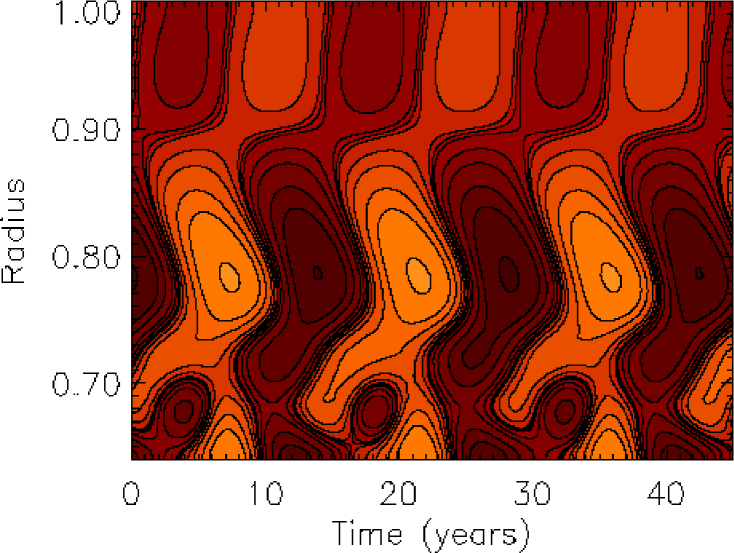
Figure 1: The radial (r–t) contours of the angular velocity residuals $\delta\Omega$ as a function of time for a cut at $25$ degrees latitude, with vacuum boundary conditions and $R_{\alpha}=-5.5,P_{r}=0.6,R_{\omega}=60000$. Note the fragmentation at the bottom of the convection zone and the resulting difference in periods of oscillations at the top and at the bottom. Darker and lighter regions represent positive and negative deviations from the time averaged background rotation rate.

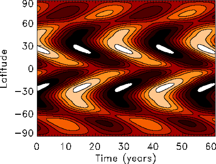
Figure 2: Butterfly diagram of the toroidal component of the magnetic field $\@vec{B}$ at $r_{0}=0.90R$, with the vacuum boundary conditions and the parameter values given by $R_{\alpha}=-5.5,P_{r}=0.6,R_{\omega}=60000$. Dark and light shades correspond to positive and negative values respectively.

We note that this is the first time STF has been obtained with vacuum boundary conditions. This is despite the fact that the range of parameter values for which STF is present for this model is rather wide, as is the case with the boundary conditions considered below. What seems to occur here is that the onset of spatiotemporal fragmentation is close to a bifurcation point, which disrupts the butterfly diagram and rather confuses the diagnosis of the situation.

4.2 Open boundary conditions (1)

We now take boundary conditions at $r=R$ to be given by Eq. (3), where $n_{2}=0$ and $n_{1}$ is varied.

In order to find the range of values of $n_{1}$ which can be considered as physically plausible, we calculated the ratio of the poloidal fluxes $F_{s}$ given by (4) as a function of $n_{1}$. The results are given in Fig. 3. To give an idea of how this ratio compares to that of models with vacuum boundary conditions, we also calculated $F_{s}$ with vacuum boundary conditions with the same parameter values as for Fig. 1, and found that $F_{s}\sim 0.25$. As can be seen from Fig. 3 this is comparable in magnitude to the values obtained with the above open boundary conditions for a wide range of values of $n_{1}$ given by $n_{1}\;\raise 1.29167pt\hbox{$<$\kern-7.5pt\raise-4.73611pt\hbox{$\sim$ }}\;\hskip-2.0pt40$.

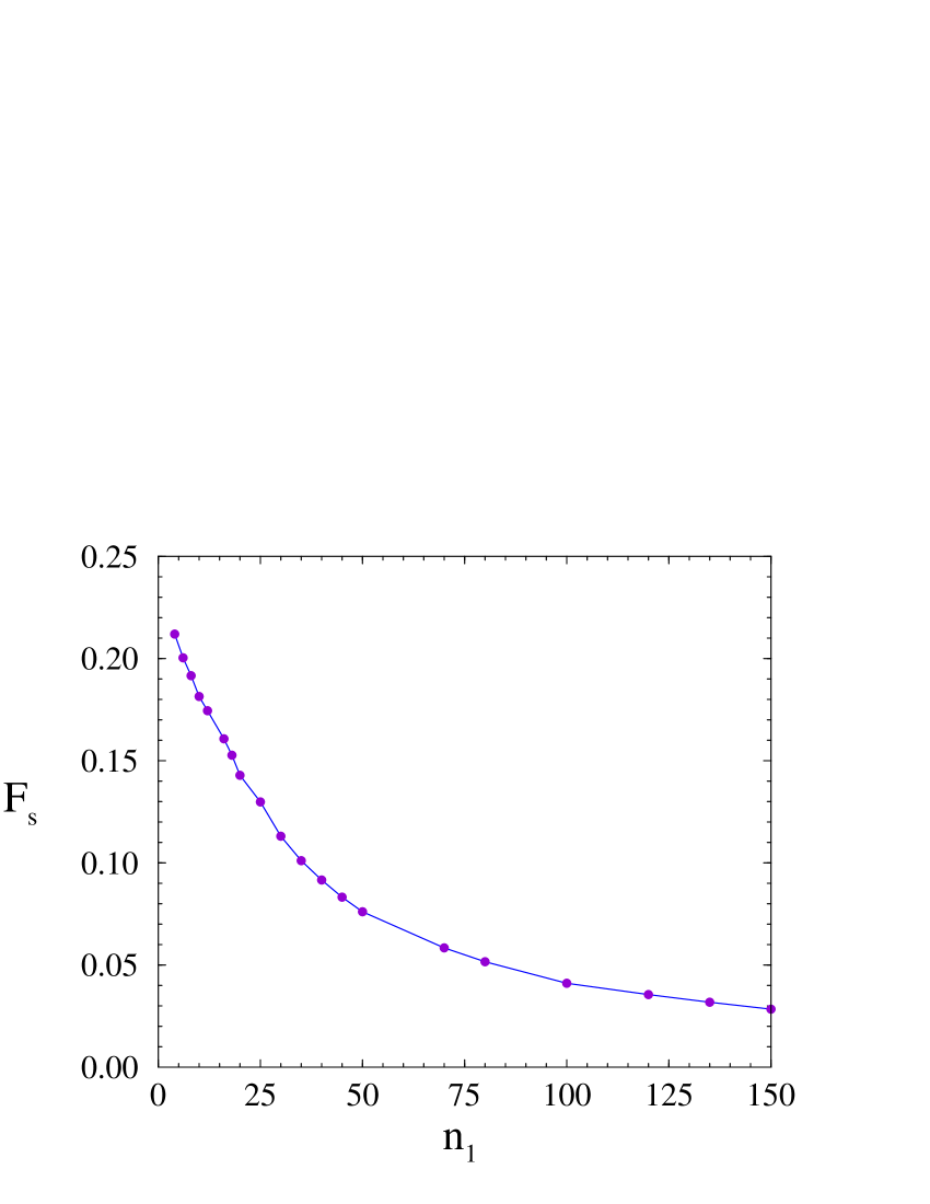
Figure 3: $F_{s}$ as a function of $n_{1}$ for the open boundary conditions (1) given by equation (3), with $n_{2}=0$.

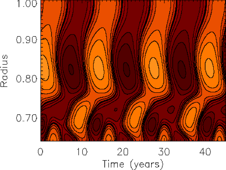
Figure 4: The radial (r–t) contours of the angular velocity residuals $\delta\Omega$ as a function of time for a cut at $25$ degrees latitude, with the boundary conditions given by (3) with $n_{1}=25$, $R_{\alpha}=-5.0,P_{r}=0.7,R_{\omega}=50000$. Note the fragmentation at the bottom of the convection zone and the resulting difference in periods of oscillations at the top and at the bottom. Darker and lighter regions represent positive and negative deviations from the time averaged background rotation rate.

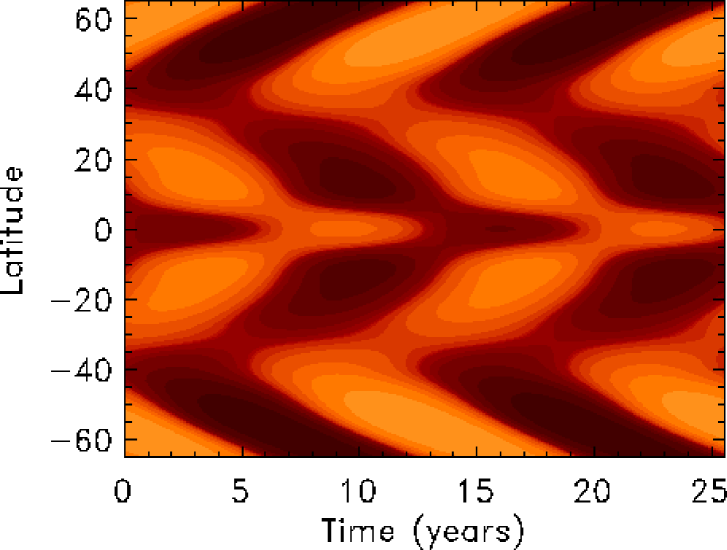
Figure 5: Angular velocity residuals at $R=0.92$ with latitude and time, with boundary conditions given by Eq. (3), $n_{1}=25$, $R_{\alpha}=-5.0,P_{r}=0.7,R_{\omega}=50000$. A temporal average has been subtracted to reveal the migrating banded zonal flows. Darker and lighter regions represent positive and negative deviations from the time averaged background rotation rate.

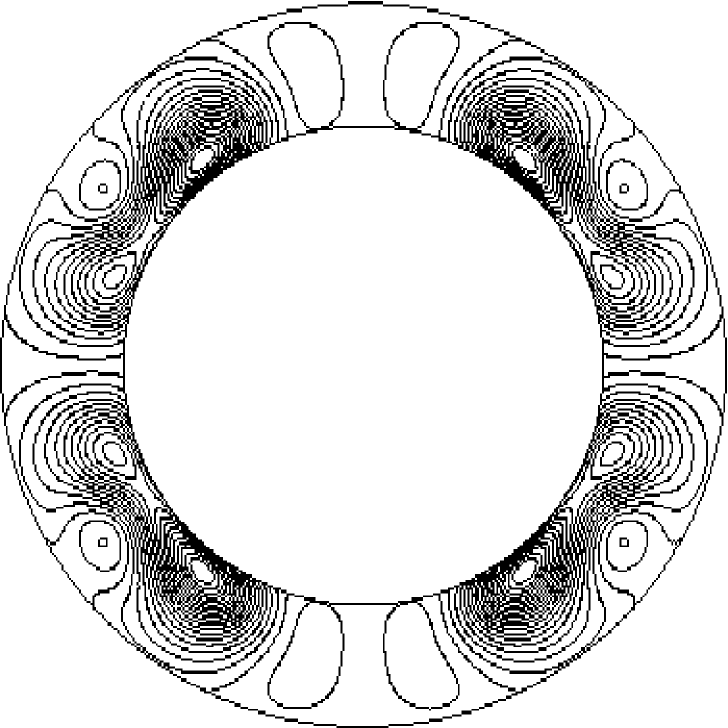
Figure 6: The poloidal field lines; same parameters as in Fig. 5.

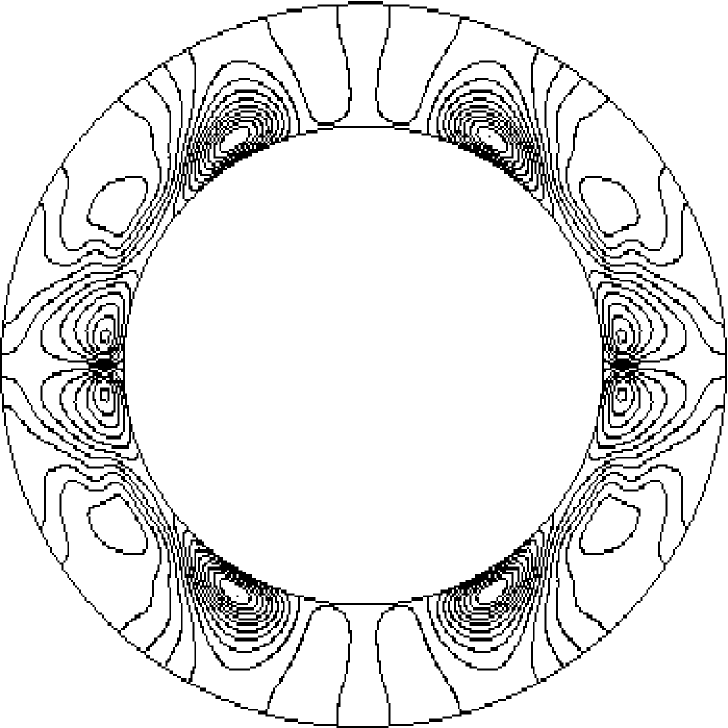
Figure 7: The toroidal field contours $\@vec{B}_{P}$; same parameters as for Fig. 5.

With these open boundary conditions, we again found that for slightly and moderately supercritical dynamo regimes, the torsional oscillations extend all the way down to the bottom of the CZ. There are also ranges of dynamo parameters for which spatiotemporal fragmentation is found. When $n_{1}$ is close to 1 there is appreciable angular momentum drift, and so we do not consider these solutions further here. As an example of a case with STF (and with negligible angular momentum drift over the integration interval), we show in Fig. 4 the radial contours of the angular velocity residuals $\delta\Omega$ as a function of time for a cut at $25$ degrees latitude. In this case $f(\theta)=\sin^{4}\theta\cos\theta$ and $\alpha_{r}$ is given by $\alpha_{r}=1$ for $0.7\leq r\leq 0.8$ with cubic interpolation to zero at $r=r_{0}$ and $r=1$. The parameter values used are $R_{\alpha}=-5.0,P_{r}=0.7,R_{\omega}=50000$ and $n_{1}=25$.

Fig. 5 shows the angular velocity residuals at $R=0.92$ (i.e. the near-surface torsional oscillations), with latitude and time, for the same parameter values as in Fig. 4. The poloidal field lines and toroidal field contours for this case are presented in Figs. 6 and 7. In Fig. 7, the effect of the open boundary condition on $B$ is seen to be relatively minor – most of the toroidal field is concentrated near the tachocline, and far from the surface. The poloidal field (Fig. 6) is more uniformly distributed.

4.3 Open boundary conditions (2)

We now consider boundary conditions given by Eq. (3), with $n_{1}$ of order one and $1\leq n_{2}\leq 500$ (so $B\approx 0$ for large $n_{2}$). We found that for $n_{1}$ values close to one our model again has significant angular momentum drift, which increases as $n_{1}$ decreases to $1$. For larger values of $n_{1}$ the drift is negligible, and the ratio $F_{s}$ is again ‘reasonable’, being comparable with the vacuum case. We found that putting $n_{1}=2$ gave satisfactory behaviour, and this is the case that we discuss in detail below.

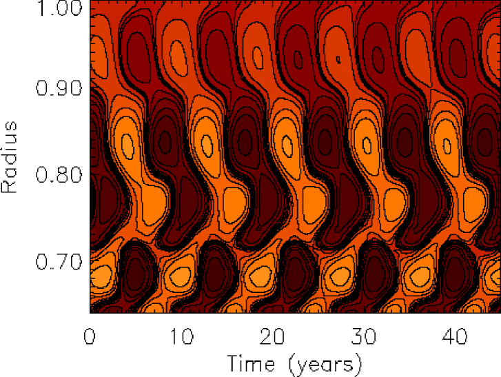
Figure 8: The radial (r–t) contours of the angular velocity residuals $\delta\Omega$ as a function of time for a cut at $20$ degrees latitude, with the open boundary conditions (2) and $R_{\alpha}=-16,P_{r}=0.22,R_{\omega}=48000$, $n_{1}=2$ and $n_{2}=400$. Note the fragmentation at the bottom of the convection zone and the resulting difference in periods of oscillations at the top and a region near the bottom of the CZ around $r_{0}=0.7$. Darker and lighter regions represent positive and negative deviations from the time averaged background rotation rate.

For all such cases we again found that for slightly and moderately supercritical dynamo numbers, the oscillations extend all the way down to the bottom of the CZ. In addition we found ranges of dynamo parameters for which the supercritical model show spatiotemporal fragmentation. An example, which has negligible angular momentum drift over the integration interval, is shown in Fig. 8. Here $\alpha_{r}=1$ for $0.7\leq r\leq 0.8$ with cubic interpolation to zero at $r=r_{0}$ and $r=1$ and $f(\theta)=\sin^{2}\theta\cos\theta$. The parameter values used were $R_{\alpha}=-16.0,P_{r}=0.22$ and $R_{\omega}=48000$, and boundary conditions were given by (3) with $n_{1}=2$ and $n_{2}=400$.

4.4 Amplitudes of oscillations as a function of boundary conditions

Another important issue from an observational point of view is the way the amplitudes of the torsional oscillations vary as a function of model ingredients and parameters, as well as with depth in the CZ.

To begin with, we verified that for a given boundary condition the amplitudes of the oscillations increase as the dynamo number $R_{\alpha}$ and the Prantdl number $P_{r}$ are increased (see also Covas et al 2001a). For orientation, we recall that the observed surface amplitudes in the case of the Sun are latitude dependent and of order of one nHz (see e.g. Howe et al. (2000b)).

We also made a comparative study of the amplitudes as a function of changes in the boundary conditions. Briefly we found that typically the solutions with vacuum boundary conditions have rather smaller amplitudes of oscillations, especially near the surface. For example, for the model of Fig. 1 (which has a high $R_{\alpha}$, spatiotemporal fragmentation and thus would be expected to have higher amplitudes), we found the mean averaged amplitudes to be $0.72,0.19,0.09$ nHz at the depths $r_{0}=0.70,0.88$ and $0.95$ respectively.

For the models with open boundary conditions, we found the amplitudes to be on average higher than the vacuum case, specially near the surface. We have summarised in Fig. 9 our calculations of the amplitudes of oscillations for the models with open boundary conditions given by Eq. (3) and $n_{2}=0$, for a range of $n_{1}$ given by $1<n_{1}<150$. Here the dynamo parameters were $R_{\alpha}=-5.0,P_{r}=0.7$, $R_{\omega}=50000$ and $f(\theta)=\sin^{4}\theta\cos\theta$, with $\alpha_{r}=1$ for $0.7\leq r\leq 0.8$, with cubic interpolation to zero at $r=r_{0}$ and $r=1$. As can be seen, the amplitudes grow at all depths with increasing $n_{1}$ and saturate around $n_{1}\sim 50$. As an example, the models with $n_{1}$ values around $n_{1}=25$, (corresponding to Fig.  4, with STF), have amplitudes that are more than double those found above with vacuum boundary conditions, down to the level $r_{0}=0.88$.

Figure 9: The mean amplitudes of torsional oscillations, at radii $r_{0}=0.70,0.88$ and $0.95$. in models with open boundary conditions given by Eq. (3) and $n_{2}=0$, with $n_{1}$ ranging from 3 to 150.

5 Discussion

We have made a detailed study of the effects of the boundary conditions on the dynamics in the solar convection zone, by employing various forms of outer boundary conditions.

In all the models considered here (as well as other results not reported), we find that in near-critical and moderately supercritical dynamo regimes the torsional oscillations extend all the way down to the bottom of the CZ. In this way our results, taken altogether, demonstrate that such penetration is extremely robust with respect to all the changes we have considered both to the boundary conditions, and the dynamo parameters such as the dynamo and Prantdl numbers, in addition to variations in the model ingredients such as the $\alpha$ and $\eta$ profiles and the rotation inversion.

We deduce, that if our dynamo model (which is basically a standard mean field dynamo) has any validity, then observers should expect to find that the solar torsional oscillations penetrate to the tachocline. However, given the significant uncertainties that still remain in helioseismic measurements, especially the limited temporal extent of the data available, this issue may not be resolvable at present (see e.g. Vorontsov et al. 2002).

In all cases we have found supercritical dynamo regimes with spatiotemporal fragmentation for a range of, but not all, dynamo parameters. This, together with our previous work, shows that fragmentation occurs with a variety of forms of $\alpha$ (and also that it is not confined to a particular inversion for the solar angular velocity). For still more supercritical dynamo regimes we find a series of spatiotemporal fragmentations, leading eventually to spatiotemporal chaos, i.e. disappearance of coherence in the dynamo regime.

These results are of potential importance in interpreting the current observations, especially given their difficulty in resolving the dynamical regimes near the bottom of the convection zone. However given the variety of dynamical behaviour possible theoretically near the bottom of the CZ, we cannot comment definitively on the reported $1-3$ yr oscillations.

Finally, given the observational importance of the amplitudes of the torsional oscillations, we have made a comparative study of their magnitudes as a function of the boundary conditions. We found that on average the amplitudes are smaller for the models with vacuum boundary conditions than for those with open boundary conditions. An important ingredient that our model omits and which seems bound to have an effect on the amplitudes of torsional oscillations throughout the CZ, is that of density stratification. We intend to return to this issue in a future publication.

- (1) Antia H.M., Basu S., 2000, ApJ, 541, 442
- (2) Covas E., Tavakol R., Moss D. & Tworkowski A., 2000a, A&A, 360, L21
- (3) Covas E., Tavakol R. & Moss D., 2000b, A&A, 363, L13
- (4) Covas E., Tavakol R. & Moss D., 2001a, A&A, 371, 718
- (5) Covas E., Tavakol R., Vorontsov, S. & Moss, D., 2001b, A&A, 375, 260
- (6) Covas E., Moss, D., & Tavakol R., 2002, Erratum, A&A, to appear
- (7) Howard R. & LaBonte B. J., 1980, ApJ Lett. 239, 33
- (8) Howe R., et al., 2000a, ApJ Lett., 533, 163
- (9) Howe R., et al., 2000b, Science, 287, 2456
- (10) Kitchatinov L.L., Mazur M. V. & Jardine M., 2000, A&A, 359, 531
- (11) Kosovichev A. G. & Schou J., 1997, ApJ, 482, 207
- (12) Moss D., Mestel L. & Tayler R.J., 1990, MNRAS, 245, 550
- (13) Moss D. & Brooke J., 2000, MNRAS, 315, 521
- (14) Rüdiger R. & Brandenburg A., 1995, A&A, 296, 557
- (15) Schou J., Antia H. M., Basu S. et al., 1998, ApJ, 505, 390
- (16) Snodgrass H. B., Howard R. F. & Webster L. 1985, Sol. Phys., 95, 221
- (17) Tworkowski A., Tavakol R., Brooke J.M., Brandenburg A., Moss D. & Tuominen, I., 1998, MNRAS, 296, 287
- (18) Vorontsov, S., Tavakol, R., Covas, E. & Moss, D., (2002) ‘Solar cycle variation of the solar internal rotation: heleioseismic inversion and dynamo modelling’, To appear in ‘Proceedings of Granada Workshop on ‘The evolving Sun and its influence on planetary environments’, ASP (Astronomical Society of the Pacific) Conference Series, A. Gimenez, E. Guinan and B. Montesinos (eds), astro-ph/0201422, also available at http://www.eurico.web.com