A Multifrequency Analysis of the Polarized Diffuse Galactic Radio Emission at Degree Scales

Abstract

The polarized diffuse Galactic radio emission, mainly synchrotron emission, is expected to be one of the most relevant source of astrophysical contamination at low and moderate multipoles in cosmic microwave background polarization anisotropy experiments at frequencies $\nu\leq 50\div 100$ GHz. We present here preliminary results based on a recent analysis of the Leiden surveys covering about 50% of the sky at low as well as at middle and high Galactic latitudes. By implementing specific interpolation methods to deal with these data, which show a large variation of the sampling across the sky, we produce maps of the polarized diffuse Galactic synchrotron component at frequencies between 408 and 1411 MHz with pixel sizes larger or equal to $\simeq 0.92^{\circ}$. We derive the angular power spectrum of this component for the whole covered region and for three patches in the sky significantly oversampled with respect to the average and at different Galactic latitudes. We find multipole spectral indices typically ranging between $\sim-3$ and $\sim-1\div-1.5$, according to the considered frequency and sky region. At $\nu\geq 610$ MHz, the frequency spectral indices observed in the considered sky regions are about $-3.5$, compatible with an intrinsic frequency spectral index of about $-5.8$ and a depolarization due to Faraday rotation with a rotation measure RM of about $15$ rad/m². This implies that the observed angular power spectrum of the polarized signal is about 85% or 20% of the intrinsic one at 1411 MHz or 820 MHz respectively.

1 Introduction

The polarized diffuse Galactic synchrotron emission, whose study provides important insights into the properties of the Galactic magnetic field and the interstellar ionized matter, is expected to be one of the most relevant source of astrophysical contamination at low and moderate multipoles in cosmic microwave background (CMB) polarization anisotropy experiments at frequencies $\nu\leq 50\div 100$ GHz. At frequencies about 1 GHz, the Galactic synchrotron emission dominates over the Bremsstrahlung emission which, although expected to be weakly polarized, significantly increases with the frequency, $\nu$, in comparison with the synchrotron one.

While ongoing and future experiments with high sensitivity and resolution are expected to cover large sky areas at different Galactic latitudes and frequencies (see, e.g., these Proceedings), the Leiden surveys [1], covering about 50% of the sky, can be used to derive the angular power spectrum of the polarized diffuse Galactic radio emission at frequencies between 408 and 1411 MHz. We have implemented specific interpolation methods to project surveys with large variations of the sampling across the sky into maps; we work here with pixel sizes larger or equal to $\simeq 0.92^{\circ}$, appropriate to the case of the Leiden surveys. Some sky areas, both at low and middle/high Galactic latitudes, show a much better sky sampling than the average and are particularly suitable for an analysis in terms of angular power spectrum. Their extents, few tens of degrees both in Galactic latitude $b$ and longitude $l$, together with the beamwidths (HPBW from $2.3^{\circ}$ to $0.6^{\circ}$ for $\nu$ from 408 to 1411 MHz) and the measure sensitivities (of about 100 mK at 610 GHz and about 1.5 (3) times better (worst) at the highest (lowest) frequency) imply that, in principle, we can study the angular power spectrum, $C_{\ell}^{ant}$ (here in terms of antenna temperature), in a multipole range from $\ell\sim$ few tens, where boundary effects begin to be neglibible, to about $\ell\sim 100$, where, even for the better sampled regions, the noise power is close to the signal power. In addition, the survey full coverage analysis allows to recover the $C_{\ell}^{ant}$s at $\ell$ between $\sim 5$ and few tens.

As a by-product of this work, these maps of polarized diffuse Galactic emission, once properly rescaled in frequency, can be used as inputs for simulation activities in current and future microwave polarization anisotropy experiments.

2 Map production and consistency tests

The main problem in the analysis of the Leiden surveys is due to their poor sampling across the sky; it is necessary to project them into maps with pixel size of about $3.7^{\circ}$ (i.e. $n_{side}=16$; we use here the HEALPix scheme [2] in which the number of pixel in the sky is $12n_{side}^{2}$), to find about one observation into each pixel of the whole observed sky region. For the same reason, a smoothing of the whole data with a window function with comparable size can not be properly applied. On the other hand, for some sky regions the sampling of the surveys is significantly much better, by a factor $\simeq 4$. We identified three regions (see [3]): patch 1 [($110^{\circ}\leq l\leq 160^{\circ}$, $0^{\circ}\leq b\leq 20^{\circ}$)]; patch 2 [($5^{\circ}\leq l\leq 80^{\circ}$, $b\geq 50^{\circ}$) together with ($0^{\circ}\leq l\leq 5^{\circ}$, $b\geq 60^{\circ}$) and ($335^{\circ}\leq l\leq 360^{\circ}$, $b\geq 60^{\circ}$)]; patch 3 [($10^{\circ}\leq l\leq 80^{\circ}$, $b\geq 70^{\circ}$)].

Therefore, we chose to derive the angular power spectrum at $\ell$ between $\simeq 5$ and $\simeq 50$, as representative of the “whole” sky, by working with the survey full coverage, and at $\ell$ between $\simeq 30$ and $\simeq 100$ by working with the above patches, which allow to analyze both low and middle/high Galactic latitudes. We anticipate that in these patches the polarized signal is typically higher than the average and it also shows relevant intensity variations on scales of some degrees. We then expect to find in the patches an angular power spectrum relatively higher than the spectrum obtained from the survey full coverage analysis in the common multipole range.

By simply averaging the survey observations in a given pixel, we can produce maps of polarized signal $P$ (and also of Stokes parameters $Q$ and $U$) that can be analyzed in terms of $C_{\ell}^{ant}$s of the polarized signal (and $E$ and $B$ modes). On the other hand, we verified that the results produced in this way, although in rather good agreement with those derived from the improved method described below both in terms of maps and of $C_{\ell}^{ant}$s, are affected by discontinuity effects on scales of the order of the pixel size. This tends to add power in the recovered $C_{\ell}^{ant}$s, particularly at multipoles close to that corresponding to the pixel size [$\ell\sim 180/(\theta_{\rm pix}/{\rm deg})$], because of its “euristic” similarity with point source confusion noise.

To overcome this problem, we implemented a specific “interpolation” method and decided to produce maps at resolution of about $0.92^{\circ}$ (in order to smooth the discontinuities discussed above on scales of about $2^{\circ}$), which, of course, provide reliable information only on scales larger than $\simeq 2^{\circ}$, i.e. only up to $\ell\simeq 100$. We assign to each sky pixel the average of the signals falling close to the pixel centre, properly weighted according to a certain power of the distance from the pixel. Different powers have been tested (from $\sim 0.5$ to $\sim 2$): clearly, the higher the power the higher the map contrast. On the other hand, we verified that the results depend very weakly on the adopted power. The algorithm searches, pixel by pixel, for a suitable number of observations to use in the weighted average, according to the following basic recipes: (i) to have enough observations (typically more than 3, if compatible with the following criteria); (ii) to use only observations quite close to the considered pixel centre (typically, less than few degrees, if compatible with the other criteria); (iii) to obtain the convergency of the result (i.e. minimize its fractional variation) with the variation of the number of observations and of the circle around the pixel centre that contain them. By applying our algorithm with different resolutions (we consider here $n_{side}$ from 16 to 64), we can test its dependence on the details of its practical application. Clearly, each interpolation method may alter the power at small scales; in principle, it operates as a kind of filter or regularization of the map and may decrease the power at small scales. Then, a reasonable agreement with the angular power spectrum derived, whenever possible, from other data with a better sampling across the sky (at the same $\nu$ and in same sky region) is crucial to probe the validity of the code recipes: in particular, for the reason discussed above, we require that it does not produce an underestimation of the power spectrum.

We obtained maps for $P$, $Q$, and $U$ at all frequencies and with different resolutions ($16\leq n_{side}\leq 64$) by using the different methods discussed above .

From each map, by using the HEALPix package (properly the “anafast” code) we derive the angular power spectrum of the polarized signal for the survey full coverage and for the three considered patches (we renormalized the $C_{\ell}^{ant}$s to the case of whole sky coverage). Preliminary results at 1411 MHz as well as tests of the applicability of this method to derive the $C_{\ell}^{ant}$s on relatively small patches have been reported in [3] (in our case the limited patch extent is a minor problem, because of the larger dimension of the considered sky areas).

In the next section we present some of our results and show how both the maps and the angular power spectra derived from them pass all the consistency tests discussed above.

3 Results

In Fig. 1 we show one of the maps of polarized signal produced with the code described in the previous section.

In Fig. 2 we compare the angular power spectra of the patch 1 at 610 MHz obtained by working at different resolutions: note the good agreement in the common multipole range. The same holds at all frequencies for the different sky regions considered here and also by extending the comparison to the lowest resolution maps ($n_{side}=16$), a crucial test in the case of the survey full coverage analysis.

The angular power spectrum derived from each map is, of course, mainly given by the sum of the astrophysical diffuse component relevant here, the synchrotron, and of the instrumental noise; in particular, the latter dominates at large multipoles, as it is evident also from the flattening we find there. We fit the recovered $C_{\ell}^{ant}$s as sum of two components, represented by a set of parameters: (i) the synchrotron component, smoothed with the beam (assumed to be perfectly symmetric and Gaussian), is approximated as $k\ell^{\alpha}{\rm exp}[-(\sigma_{b}\ell)^{2}]$, $\sigma_{b}$ being the 1$\sigma$ beamwidth (of course, the window function is not crucial in this context at the highest frequencies); (ii) the noise contribution is approximated as a flat, white noise, component, $c_{wn}$. All the parameters of the fit depend on $\nu$ and on the sky region. In each case, we find the best fit parameters at $\ell$ between $\sim 30$ and $\sim 100\div 200$; we separately repeat the fit at $\ell$ between $\sim 5$ and $\sim 30$ in the case of the survey full coverage analysis.

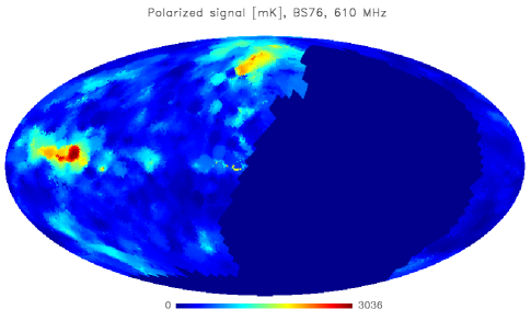
Figure 1: Map of polarized signal obtained at $n_{side}=64$ ($\simeq 0.92^{\circ}$ of pixel size).

Figure 2: Comparison between the angular power spectra obtained by projecting the Leiden surveys into maps at different resolution, $n_{side}=32$ (i.e., pixel size $\simeq 1.8^{\circ}$, dotted line) and 64 (i.e., pixel size $\simeq 0.92^{\circ}$, solid line).

Of course, it is extremely important to check that the level of the noise power derived from the fit is similar to that derived on the basis of the rms noise per pixel in the map. Given rms noise maps, we generate simulated maps of white noise and extract their $C_{\ell}^{ant}$s. This is shown in Fig. 3. We quote the rms noise per pixel by using three different methods: (i) the rms noise calculated by using the rms noise of each observation and propagating the error according to the mathematical rules applied to produce the maps (solid lines); (ii) the same as in the case (i), except for pixels in which survey observations fall, in which case we apply the standard weighted error on the standard weigthed average (dot-dashed line in the left panel); (iii) the standard weighted error on the standard weigthed average for pixels in which survey observations fall, and the average of these errors for the other pixels (three dots-dashes). Of course, for the patches, and particularly for the patch 3, the evaluations (ii) and (iii) provide practically the same results, given the good sampling across the sky; thus, we only report the evaluation (iii). Note that, for the survey full coverage analysis, the noise spectrum evaluated according to (iii) is of the order of that derived from the signal map at $\ell\sim 50$: therefore, at $\ell$ larger than $\sim 50$ no reliable information can be derived. For the patches, on the contrary, the noise spectrum is below that derived from the signal map, independently of the different noise evaluations, up to $\ell\sim 100$. This confirms that, not only from the point of view of the sampling across the sky, but also from the point of view of the sensitivity, the patches can be used to extract the synchrotron $C_{\ell}^{ant}$s up to $\ell\sim 100$. We note that this is not valid, in principle, for possible analyses of patches in other sky regions less sampled and of lower polarized signal intensity, where we expect a signal to noise ratio close to that derived here for the survey full coverage analysis, i.e. a reliable information can be obtained only up to $\ell\sim 50$.

From the survey full coverage analysis, we derive reliable information also at $5\leq\ell\leq 30$ (of course, only nearly full sky observation can provide reliable information at very low multipoles). In this case, both the noise and possible effects introduced by the poor sampling or by the adopted “interpolation” technique are clearly negligible. We find a flattening of the spectrum with respect to that at higher multipoles; the slope (dotted line of left panel of Fig. 3) at $\nu=1411$ MHz, crucial for the extrapolation to higher frequencies, is close to $-2.5$. This implies an essentially flat (slope $\sim-0.25$) behaviour of $\delta T_{\ell}=\sqrt{\ell(2\ell+1)C_{\ell}/4\pi}$ at $5\leq\ell\leq 30$ ($\delta T_{\ell}$ is a quantity particularly relevant in the comparison with the CMB temperature and polarization anisotropy observations).

Figure 3: Angular power spectra derived from the map (thin solid lines) and synchrotron (thick solid lines) and synchrotron plus noise (thick dot-dashed lines) best fit spectra at multipoles larger than $\sim 30$ compared with the those derived from simulated maps of pure white noise with different estimates of the rms noise per pixel (roughly horizontal lines). In the case of the survey full coverage analysis we report also the $C_{\ell}^{ant}$s obtained at lower multipoles (again, thin solid line) together with the best fit spectrum (dotted line) dominated by the synchrotron component (see also the text).

We focus now on the angular power spectrum of the synchtrotron component at $\ell$ between $\simeq 30$ and $\simeq 100\div 200$. Our results are summarized in Fig. 4. We find slopes varying from about $-3$ to about $-1\div-1.5$, mainly depending on the frequency, although, as expected, different sky regions show different slopes even at the same frequency.

As already recognized (see [3]), we find a particularly impressive agreement between the result obtained for the patch 1 and the angular power spectrum (long dashes in Fig. 4) obtained at 1411 MHz in a smaller region (the region 2 in eq. (20) of [3]) inside the patch 1 by exploiting the data from [4] (which have better sampling across the sky, sensitivity and resolution and in which only the absolute calibration takes advantage of the Leiden surveys). This strongly supports the validity of our code to project the Leiden surveys into HEALPix maps or, at least, indicates that it does not introduce significant errors in the evaluations of the $C_{\ell}^{ant}$s even at $\ell\sim 100$ and in the worst case of $\nu=1411$ MHz (here the ratio between the beamwidth and the typical angular distance among adjacent survey pointings is minimal and the survey sky coverage is not the best – it occurs at 610 MHz).

Figure 4: Synchrotron component of the angular power spectrum derived for the entire map and the three patches at the different frequencies: 408 (solid lines), 465 (dotted lines), 610 (dashed lines), 820 (dot-dashed lines) and 1411 MHz (three dots-dashes). In the case of the patch 1, note the good agreement (within a factor $\sim 2$) with the spectrum (long dashes) obtained from a smaller patch inside the patch 1 by exploiting the survey [4] at 1411 MHz (see also the text).

4 Discussion and Conclusions

We presented here preliminary results based on a recent analysis of the Leiden surveys for about 50% of the sky and three patches at low as well as at middle/high Galactic latitudes significantly better sampled than the average. By implementing specific interpolation methods, we produce maps of the polarized diffuse Galactic synchrotron component at frequencies between 408 and 1411 MHz with pixel sizes larger or equal to $\simeq 0.92^{\circ}$.

We derive the angular power spectrum of the polarized diffuse Galactic synchrotron emission for the whole covered region and for the three patches. The multipole spectral indices typically range between $\sim-3$ and $\sim-1\div-1.5$, depending on the frequency and on the sky region.

Together with the large sky coverage, the multifrequency Leiden surveys offer the opportunity to study the dependence of the Galactic synchrotron polarized signal on $\nu$. Clearly, depolarization effects and possible transitions from essentially optically thin regimes to significantly self-absorbed ones may “obscure” the intrinsic synchrotron spectral behaviour. We find large variations of the spectral index observed in the different sky pixels, probably due to real variations, but also to the limited sensitivity and, perhaps, to differential depolarization effects related to the $\nu$-dependent beamwidth or, finally, to possible systematic and not well understood effects in the data. We try to circumvent, at least in part, these difficulties by exploiting the “statistical” information contained in the $C_{\ell}^{ant}$s.

In Fig. 5 we show the angular power spectrum as a function of $\nu$ at the multipole $\ell=50$ (a middle, representative value considered in this study); we find very similar results also at $\ell=30$ and 100. The observed frequency spectral indices at $\ell=50$ are $\sim$ $-3.2$ (survey full coverage analysis), $-3.3$ (patch 1), $-3.6$ (patch 2) and $-3.9$ (patch 3). At the highest frequencies (820, 1411 MHz), that are crucial for the extrapolation at frequencies of $20\div 100$ GHz relevant for CMB anisotropy polarization radiometric experiments and where beamwidth depolarization effects are expected to be quite similar (HPBW varying only of $\sim 50$% between 820 and 1411 MHz), the observed slope can be easily explained by assuming an intrinsic slope of $-5.8$ (as in the case of a slope $-0.9$ in terms of flux) and a depolarization due to Faraday rotation with a rotation measure RM of about $15$ rad/m². This results is in quite good agreement with that previously obtained from the analysis of a sky region partially overlapped with the patch 1, as well as clearly compatible with the upper limits on RM found in the Leiden surveys (see [5]). This implies that the observed angular power spectrum of the polarized signal is about 85% or 20% of the intrinsic one (strictly, in absence of Faraday rotation depolarization) at 1411 MHz or 820 MHz respectively.

Figure 5: Angular power spectrum at multipole $\ell=50$ as function of $\nu$ for the different sky regions: the survey full coverage (solid lines), the patch 1 (dotted lines), the patch 2 (dashed lines) and the patch 3 (dot-dashed lines). The straight longer lines represent a simple power law dependence of the $C_{\ell}^{ant}$s (at $\ell=50$) on $\nu$ corresponding to an “intrinsic” slope of $-5.8$, rescaled to the angular power spectra derived here at 1411 MHz. The straight shorter lines represent the dependence of the $C_{\ell}^{ant}$s on $\nu$ between 820 and 1411 MHz for a Faraday rotatation depolarization with RM = 15 rad / m² applied to the above “intrinsic” slope (in the case of the survey full coverage analysis, note the practically perfect agreement with the observed spectrum between 820 and 1411 MHz). Note also the further flattening of the spectrum at the lowest frequencies in the case of the two patches at relatively high Galactic latitudes (see also the text).

5 References

1. Brouw W.N., Spoelstra T.A.T., A&AS, 26, 129 (1976)

2. Gòrski K.M., Hivon E., Wandelt B.D. 1998, “Analysis Issues for Large CMB Data Sets”, in MPA/ESO Conference on Evolution of Large-Scale Structure: from Recombination to Garching, edited by A.J. Banday, R.K. Sheth, L. Da Costa, 37, astro-ph/9812350

3. Baccigalupi C., Burigana C., Perrotta F., et al., A&A, 372, 8 (2001)

4. Uyaniker B., Furst E., Reich W., Reich P., Wielebinski R., A&AS, 138, 31 (1999)

5. Spoelstra T.A.T., A&A, 135, 238 (1984)