How to Construct a GRB Engine?

Tsvi Piran and Ehud Nakar
Racah Institute for Physics
The Hebrew University
Jerusalem, ISRAEL

1 Introduction

Our understanding of Gamma-Ray Bursts (GRBs) was revolutionized during the last ten years. According to the generally accepted Fireball model (see e.g. [1, 2]) the gamma-rays and their subsequent multiwavelength afterglow are produced when an ultra-relativistic flow is slowed down. All current observations, from prompt emission to late afterglow, from $\gamma$-rays via X-ray optical and IR to radio, are consistent with this model.

Observations of GRB host galaxies revealed the association of (long) GRBs (there is no information on the positions of short GRBs) with star forming Galaxies [3] and that these (long) GRBs follow the star formation rate [4, 5, 6]. There is evidence (still inconclusive) that some long bursts are associated with Supernovae [7, 8, 9, 10]. These observations suggest that the progenitors of GRBs are massive stars. There are some reasonable ideas how does a collapsing star [11, 12, 13] or a merging binary [14] produce the required $\sim 10^{51}$ergs. But it is not clear how does the GRB’s “inner engine” accelerates and collimated the relativistic flow. Today this is the most interesting (and most difficult) open question concerning GRBs. This is also the most relevant question for this conference where the possibility that transitions to strange stars power GRBs has been discussed [15].

We summarize, here, the known constrains on the “inner engines” of GRBs. These constrains arise mostly from the temporal structure of GRBs. Several years ago Sari and Piran [16] have shown that variable GRBs can be generated only by internal interactions within the flow. To produce internal shocks the central engine must produce a long and variable wind. This leads to a powerful NO GO theorem: Variable GRBs cannot be produced from a single explosion. This NO GO theorem rules out explosive GRB models that produce the relativistic flow in a single explosion. Kobayashi et al [17] have shown that the observed internal shocks light curve reflects almost directly the temporal activity of the inner engine. This is the best direct evidence on what is happening at the center of the GRB.

We review the arguments leading to these conclusions. We also discuss new observational results [18, 19, 20] and a new theoretical toy model [21] that explains these observations within the internal shocks paradigm. This toy model suggests that the “inner engine” is producing a variable Lorentz factor wind by modulating the mass ejection of a roughly constant energy flow. The other alternative of modulating the energy of a constant mass flow is ruled out. We conclude by summarizing the various constrains on the “inner engines”. We leave to the reader the task of examining the implications of these results to his/hers favorite model.

2 Energetics and Beaming

The most important factor in any model is the total amount of energy that it releases. Redshift measurements have lead to alarming estimates of more than $10^{54}$ergs in some bursts [23]. When factoring in the efficiency the requirements exceed a solar rest mass energy.

However, these early estimates assumed isotropic emission. Jet breaks in afterglow light curves lead to estimates of the beaming factors. When those are taken into account we find a “modest” practically constant energy release of $\sim 10^{51}$ergs [24, 25, 26, 27]. This lower energy budget allows for many possible models. At the same time it introduces an additional requirement on the central engine. It has to collimate the relativistic flow to narrow beaming angles (at times or order of $1^{o}-2^{o}$).

We cannot estimate directly the total energy released by the “inner engine”. However, here are two possible estimates: $E_{\gamma}$, the energy released as $\gamma$-rays and $E_{K}$, the kinetic energy during the adiabatic afterglow phase. Remarkably both energies are comparable. This last observation implies that the conversion efficiency of the initial relativistic kinetic energy to $\gamma$-rays must be very high.

3 Time Scales In GRBs - Observations

Most GRBs are highly variable. Fig 1 depicts the light curve of a typical variable GRB (GRB920627). The variability time scale, $\delta t$, is determined by the width of the peaks. $\delta t$ is much shorter (in some cases by a more than a factor of 100) then $T$, the duration of the burst. Variability on a time scale of milliseconds is seen in some long bursts [20]. However, not all bursts are variable. We stress that our discussion applies to variable bursts and it is not applicable to the small subset of smooth ones.

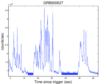
Figure 1: The light curve of GRB920627. The total duration of the burst is 52sec, while typical pulses are 0.8sec wide. Two quiescent periods lasting $\sim$10 seconds are marked by horizontal solid bold lines.

A comparison of the pulse width distribution and the pulse separation, $\Delta t$ , distribution, reveals an excess of long intervals [18, 19]. These long intervals can be classified as quiescent periods [28], relatively long periods of several dozen seconds with no activity. When excluding the quiescent periods we [18, 19] find that both distributions are lognormal with a comparable parameters: The average pulse interval, $\overline{\Delta}t=1.3sec$ is larger by a factor 1.3 then the average pulse width $\overline{\delta}t=1sec$. One also finds that the pulse widths are correlated with the preceding interval [18, 19].

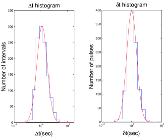
Figure 2: The pulse width distribution (right) and the distribution of intervals between pulses (left) (from [19]).

The results described so far are for long bursts. the variability of short ($T<2$sec) bursts is more difficult to analyze. The duration of these bursts is closer to the limiting resolution of the detectors. Still we find that most ($\sim 66\%$) short bursts are variable with $\delta t/T<0.1$ [20].

4 Time Scales In GRBs - Theory

Consider a spherical relativistic emitting shell with a radius $R$, a width $\Delta$ and a Lorentz factor $\Gamma$. This can be a whole spherical shell or a spherical like section of a jet whose opening angle $\theta$ is larger than $\Gamma^{-1}$. Because of relativistic beaming an observer would observe radiation only from a region of angular size $\Gamma^{-1}$. Photons emitted by matter moving directly towards the observer (point A in Fig. 3) will arrive first. Photons emitted by matter moving at an angle $\Gamma^{-1}$ (point D in Fig. 3) would arrive after $t_{ang}=R/2c\Gamma^{2}$. This is also the time of arrival of photons emitted by matter moving directly towards the observer but emitted at $2R$ (point C in Fig. 3). Thus, $t_{rad}\approx t_{ang}$ [16, 29]. This coincidence is the first part of the NO GO theorem that rules out single explosions a sources of GRBs.

Figure 3: Different time scale from a relativistic expanding shell in terms of the arrival times ($t_{i}$) of various photons: $t_{ang}=t_{D}-t_{A}$, $t_{rad}=t_{C}-t_{A}$ and $T_{\Delta}=t_{B}-t_{A}$.

At a given point particles are continuously accelerated and emit radiation as long as the shell with a width $\Delta$ is crossing this point. The photons emitted at the front of this shell will reach the observer a time $T_{\Delta}=\Delta/c$ before those emitted from the rear (point B in Fig. 3). In fact photons are emitted slightly longer as it takes some time for the accelerated photons to cool. For most reasonable parameters the cooling time is much shorter from the other time scales [30] and we ignore it hereafter.

Light curves are divided to two classes according to the ratio between $T_{\Delta}$ and $t_{ang}\approx t_{rad}$. The emission from different angular points smoothes the signal on a time scale $t_{ang}$. If $T_{\Delta}\leq t_{ang}\approx t_{rad}$ the resulting burst will be smooth with a width $t_{ang}\approx t_{rad}$. The second part of the NO GO theorem follows from the hydrodynamics of external shocks. Sari and Piran [16] have shown that for external shocks $\Delta/c\leq R/c\Gamma^{2}\approx t_{rad}\approx t_{ang}$. External shocks can produce only smooth bursts!

A necessary condition for the production of a variable light curve is that $T_{\Delta}=\Delta/c>t_{ang}$. This can be easily satisfied within internal shocks (see Fig 4). Consider an “inner engine” emitting a relativistic wind active over a time $T_{\Delta}=\Delta/c$ ($\Delta$ is the overall width of the flow in the observer frame). The source is variable on a scale $L/c$. The internal shocks will take place at $R_{s}\approx L\Gamma^{2}$. At this place the angular time and the radial time satisfy: $t_{ang}\approx t_{rad}\approx L/c$. Internal shocks continue as long as the source is active, thus the overall observed duration $T=T_{\Delta}$ reflects the time that the “inner engine” is active. Note that now $t_{ang}\approx L/c<T_{\Delta}$ is trivially satisfied. The observed variability time scale in the light curve, $\delta t$, reflects the variability of the source $L/c$. While the overall duration of the burst reflects the overall duration of the activity of the “inner engine”.

Numerical simulations [17] have shown that not only the time scales are preserved but the source’s temporal behaviour is reproduced on an almost one to one basis in the observed light curve. We will return to this point in section 6 in which we describe a simple toy model that explains this result.

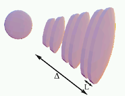
Figure 4: The internal shocks model (from [32]). Faster shells collide with slower ones and produce the observed $\gamma$ rays. The variability time scale is $L/c$ while the total duration of the burst is $\Delta/c$ .

5 Caveats and Complications

Clearly the way to get around the NO GO theorem is if $t_{ang}<t_{rad}$. In this case one can identify $t_{rad}$ with the duration of the burst and $t_{ang}$ as the variability time scale. The observed variability would require in this case that: $t_{ang}/t_{rad}=\delta t/T$.

One can imagine an inhomogeneous external medium which is clumpy on a scale $d\ll R/\Gamma$ (see Fig 5). Consider such a clump located at an angle $\theta\sim\Gamma^{-1}$ to the direction of motion of the matter towards the observer. The resulting angular time, which is the difference in arrival time between the first and the last photons emitted from this region would be:$\sim d/c\Gamma$. Now $t_{ang}<t_{rad}$ and it seems that one can get around the NO GO theorem.

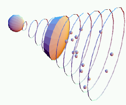
Figure 5: The clumpy ISM model (from [32]). Note the small covering factor and the resulting “geometrical” inefficiency.

Sari and Piran [16] have shown that such a configuration would be extremely inefficient. This third component of the NO GO theorem rules out this caveat. The observations limit the size of the clumps to $d\approx c\Gamma\delta t$ and the location of the shock to $R\approx cT\Gamma^{2}$. The number of clumps within the observed angular cone with an opening angle $\Gamma^{-1}$ equals the number of pulses which is of the order $T/\delta t$. The covering factor of the clumps can be directly estimated in terms of the observed parameters by multiplying the number of clumps $T/\delta t$ times their area $d^{2}=(\delta t\Gamma)^{2}$ and dividing by the cross section of the cone $(R/\Gamma)^{2}$. The resulting covering factor equals $\delta t/T\ll 1$. The efficiency of conversion of kinetic energy to $\gamma$-rays in this scenario is smaller than this covering factor which for a typical variable burst could be smaller than $10^{-2}$.

We turn now to several attempts to find a way around this result. We will not discuss here the feasibility of the suggested models (namely is it likely that the surrounding matter will be clumpy on the needed length scale [31], or can an inner engine eject “bullets” [33] or “cannon balls” [34] with an angular width of $\sim 10^{-2}$ degrees and what keeps these bullets so small even when they are shocked and heated). We examine only the question whether the observed temporal structure can arise within these models.

5.1 External Shocks on a Clumpy Medium

Dermer and Mitman [31] claim that the simple efficiency argument of Sari and Piran [16] was flawed. They point out that if the direction of motion of a specific blob is almost exactly towards the observer the angular time would be of order $d^{2}/cR$. This is narrower by a factor $d\Gamma/R$ than the angular time across the same blob that is located at a typical angle of $\Gamma^{-1}$. These special blobs would produce strong narrow peaks and will form a small region along a narrow cone with a larger covering factor. Dermer and Mitman [31] present a numerical simulation of light curves produced by external shocks on a clumpy inhomogenous medium with $\delta t/T\sim 10^{-2}$ and efficiencies of up to $\sim 10$%.

A detailed analysis of the light curve poses, however, several problems for this model. While this result is marginal for bursts with $\delta t/T\sim 10^{-2}$ it is insufficient for bursts with $\delta t/T\sim 10^{-3}$. Variability on a time scale of milliseconds is observed [20] in many long GRBs (namely $\delta t/T$ can be as samll as $10^{-4}$.). Moreover, in this case we would expect that earlier pulses (that arise from blobs along the direction of motion) would be narrower than latter pulses. This is in a direct contradiction with the observations [35]. Finally there is no reason to expect the observed similarity between the pulse width and the pulse separation and the correlation between the pulse width and the preceding interval in this model.

5.2 The Shot-Gun and the Cannon Ball Models

Heinz and Begelman [33] suggested that the “inner engine” operates as a shot-gun emiting multiple narrow bullets with an angular size much smaller than $\Gamma^{-1}$ (see Fig 6). These bullets do not spread while propagating and they are slowed down rapidly by an external shock with a very dense circumburst matter. The pulses width is $t_{ang}$ or the slowing down time while the duration of the burst is determined by the time that the “inner engine” emits the bullets. While the cannon ball model of Dar and De Rujulla [34] is drastically different from a physical point of view it is rather similar in terms of its temporal features. Hence the following remarks apply to this model as well.

Figure 6: The shot-gun or the cannon-ball models (from [32]). The inner engine emits narrow “bullets” that collide with the ISM.

This model satisfies our NO GO theorem in the sense that also here the burst is not produced by a single explosion. Moreover the observed light curve represents also here the temporal activity of the source. However, it is based on external shocks.

The most serious problem is the fact that the width of the pulses here is determined by the angular time or the hydrodynamic time (which in turn depends on the external density profile of the circumburst matter) while the intervals between the pulses depend on the activity of the inner engine. There is no reason why the two distributions will be similar and why there should be a correlation between them.

6 An Internal Shocks Toy Model

The discovery [18, 19] that the distribution of pulse widths and pulse separations are comparable and that there is a correlation between the pulse width and the preceding interval provides an independent evidence in favor of the internal shocks model. Furthermore it suggests that the different shells emitted by the internal engine are most likely “equal energy” rather than “equal mass” shells.

The similarity between the pulse width and the pulse separation distribution and the correlation is extremely unlikely to arise from a single shell passing thought a random distribution of clumps that surround the “central engine”. In this case the arrival time of individual pulses will depend on the position of the emitting clumps relative to the observers. Two following pulses could arise from two different clumps that are rather distant from each other. There is no reason why the pulses and intervals should be correlated in any way. A similar problem arises in the “shot-gun” or the “cannon-ball” models in which the pulse duration is determined by one parameter and the separation by another.

Both features arise naturally within the internal shocks model [21] in which both the pulse duration and the separation between the pulses are determined by the same parameter. We outline here the main arguments showing that. Consider two shells with a separation $L$. The slower outer shell Lorentz factor is $\Gamma_{1}=\Gamma$ and the inner faster shell Lorentz factor is $\Gamma_{2}=a\Gamma$ ($a>2$ for an efficient collision), both in the observer frame. The shells’ are ejected at $t_{1}$ and $t_{2}\approx t_{1}+L/c$. The collision takes place at a radius $R_{s}\approx 2\Gamma^{2}L$ (Note that $R_{s}$ does not depend on $\Gamma_{2}$). The emitted photons from the collision will reach the observer at time (omitting the photons flight time, and assuming transparent shells):

$$t_{o}\approx t_{1}+R_{s}/(2c\Gamma^{2})\approx t_{1}+L\approx t_{2}\ .$$ (1)

The photons from this pulse are observed almost simultaneously with a (hypothetical) photon that was emitted from the “inner engine” together with the second shell (at $t_{2}$). This explains why Kobayashi et al [17] find numerically that for internal shocks the observed light curve replicates the temporal activity of the source.

Consider now four shells emitted at times $t_{i}$ ($i=1,2,3,4$) with a separation of the order of $L$ between them. Assume that there are two collisions - between the first and the second shells and between the third and the fourth shells. The first collision will be observed at $t_{2}$ while the second one will be observed at $t_{4}$. Therefore, $\Delta t\approx t_{4}-t_{2}\approx 2L/c$. Now assume a different collision scenario, the second and the first shells collide, and afterward the third shell takes over and collide with them (the forth shell does not play any roll in this case). The first collision will be observed at $t_{2}$ while the second one will be observed at $t_{3}$. Therefore, $\Delta t\approx t_{3}-t_{2}\approx L/c.$ Numerical simulations [21] show that more then 80% of the efficient collisions follows one of the two scenarios described above. Therefore we can conclude:

$$\Delta t\approx L/c\ .$$ (2)

Note that this result is independent of the shells’ masses.

The pulse width is determined by the angular time (ignoring the cooling time): $\delta t=R_{s}/(2c\Gamma^{2}_{s})$ where $\Gamma_{s}$ is the Lorentz factor of the shocked emitting region. If the shells have an equal mass ($m_{1}=m_{2}$) then $\Gamma_{s}=\sqrt{a}\Gamma$ while if they have equal energy ($m_{1}=am_{2}$) then $\Gamma_{s}\approx\Gamma$. Therefore:

$$\delta t\approx\left\{\begin{array}[]{r@{\quad\quad}l}R_{s}/2a\Gamma^{2}c\approx L/ac&\rm{equal\ mass},\\ R_{s}/2\Gamma^{2}c\approx L/c&\rm{equal\ energy}.\end{array}\right.$$ (3)

The ratio of the Lorentz factors $a$, determines the collision’s efficiency. For efficient collision the variations in the shells Lorentz factor (and therefore $a$) must be large.

It follows from Eqs. 2 and 3 that for equal energy shells the $\Delta t$-$\delta t$ similarity and correlation arises naturally from the reflection of the shells initial separation in both variables. However, for equal mass shells $\delta t$ is shorter by a factor of $a$ than $\Delta t$. Since $a$ has a large variance this would wipes off the $\Delta t$-$\delta t$ correlation. This suggests that equal energy shells are more likely to produce the observed light curves.

7 Conclusions

We cannot provide a recipe for a GRB “inner engine”. However we can list the specifications of this engine (for a long variable GRB). It must satisfy the following conditions:

• It should accelerate $\sim 10^{51}$ergs to a variable relativistic flow with $\Gamma>100$.

• It should collimate this flow, with a varying degree of collimation (up to $1^{o}$).

• It should be active from several seconds up to several hundred seconds (according to the duration of the observed burst).

• It should vary on a time scale of seconds or less (corresponding to the duration of a typical pulse within the burst).

• Different shells of matter should have a comparable energy and their different Lorentz facors should arise due to a modulation of the accelerated mass.

• At times the engine should stop for several dozen seconds (resulting in a quiescent periods).

Before concluding we stress that these specification are for long variable burst (which compose the majority of the observed bursts). Many of these (but not all) apply also to short variable bursts (about two thirds of the short bursts). These specifications do not apply to smooth bursts (either short or long ones).

This research was supported by a grant from the US-Israel Binational Science Foundation.

References

- [1] T. Piran, Physics Reports, 314, 575 (1999).
- [2] T. Piran, Physics Reports, 333, 529 (2000).
- [3] A. S. Fruchter, et al., ApJ, 516, 683, (1999).
- [4] R. Wijers, J. Bloom, J. Bagla and P. Natarjan, MNRAS, 294, L13, (2000).
- [5] T. Totani, ApJ, 511, 41 (1999).
- [6] A. Blain and P. Natarajan, MNRAS, 312, L35, (2000).
- [7] T. Galama et al., Nature, 395, 70, (1998).
- [8] Bloom, J. S. et al., Nature, 401, 453 (1999).
- [9] Reichart, D. E. 1999, ApJ, 521, L111, (1999).
- [10] Galama, T. J. et al., ApJ, 536, 185 (2000).
- [11] S. E. Woosley, Ap. J., 405, 273 (1993).
- [12] B. Paczynski, Ap. J. Lett., 494, L45 (1998).
- [13] A. I. MacFadyen and S. E. Woosley, Ap. J., 524, 262 (1999).
- [14] D. Eichler, M. Livio, T. Piran, and D. N. Schramm, Nature, 340, 126 (1989).
- [15] R. Ouyed, “Quark Stars and Color Superconductivity: A GRB connection?” this volume, astro-ph/0201408 (2002).
- [16] R. Sari and T. Piran, Ap. J., 485, 270 (1997).
- [17] S. Kobayashi, T. Piran, and R. Sari, Ap. J., 490, 92 (1997).
- [18] E. Nakar and T. Piran, astro-ph/0103011, GRBs in the Afterglow Era, Eds. E. Costa, F. Fronteira and K. Hjorth,NK01,NK02a (Springer) (2001).
- [19] E. Nakar and T. Piran, MNRAS, in press, astro-ph/0103210 (2002)
- [20] E. Nakar and T. Piran, MNRAS, in press, astro-ph/0103192 (2002)
- [21] E. Nakar and T. Piran, submitted astro-ph/0202404 (2002).
- [22] R. Narayan, T. Piran and P. Kumar, Ap. J., 557, 949, (2001).
- [23] S. R. Kulkarni et al., Nature, 398, 389 (1999).
- [24] T. Piran, P. Kumar. A. Panaitescu and L. Piro, Ap. J. Lett., 560, L167, (2001).
- [25] T. Piran, astro-ph/0111314 talk given at the J. van Paradijs Memorial Symposium, June 6-8 Amsterdam, (2001).
- [26] A. Panaitescu and P. Kumar, Ap. J. Lett., 560, L49, (2001).
- [27] D. A. Frail et al., Ap. J. Lett., 562, L55 (2001).
- [28] E. Ramirez-Ruiz, and A Melroni, MNRAS, 320, K25 (2001).
- [29] E. E. Fenimore, C. D. Madras, and S. Nayakshin, Ap. J., 473, 998, (1996).
- [30] R. Sari, R. Narayan and T. Piran, Ap. J., 473, 204, (1996).
- [31] C. D. Dermer, and K. E., Mitman, Ap. J., 513, 5, (1999)
- [32] R. Sari, PhD thesis, (1998)
- [33] S. Heinz, and M. C. Begelman, Ap. J. Lett., 527, L35, (1999).
- [34] A. Dar and A. De Rujula, unpublished astro-ph/0008474 (2000).
- [35] E. Ramirez-Ruiz, and E. E. Fenimore A & A.S. 132, 521, (1999).