GRBs Light Curves - Another Clue on the Inner Engine

Abstract

The nature of the ‘inner engine’ that accelerate and collimate the relativistic flow at the cores of GRBs is the most interesting current puzzle concerning GRBs. Numerical simulations have shown that the internal shocks’ light curve reflects the activity of this inner engine. Using a simple analytic toy model we clarify the relations between the observed $\gamma$-rays light curve and the inner engine’s activity and the dependence of the light curves on the inner engine’s parameters. This simple model also explains the observed similarity between the observed distributions of pulses widths and the intervals between pulses and the correlation between the width of a pulse and the length of the preceding interval. Our analysis suggests that the variability in the wind’s Lorentz factors arises due to a modulation of the mass injected into a constant energy flow.

1 Introduction

According to the current Fireball model a Gamma-Ray Burst (GRB) contain four stages: (i) A catastrophic event produces an ‘inner pine engine’. (ii) This ‘inner engine’ accelerates a barionic wind into a highly relativistic motion. (iii) Internal collisions within this wind produce the prompt $\gamma$-ray emission (iv) An external-shock between the wind and the surrounding matter produces the afterglow. The most mysterious part of this process is the nature of the ‘inner engine’. There are no direct observations of the ‘inner engine’.

Numerical simulations (Kobayashi, Piran & Sari 1997; Ramirez & Fenimore, 2000) revealed that the $\gamma$-rays light curve replicates the temporal activity of the ’inner engine’. In this letter we explain, using a simple analytic toy model, these results. In our toy model the relativistic wind is described as a sequence of discrete shells with various Lorentz factors, $\gamma$. The $\gamma$-rays light curve results from collisions between shells with different values of $\gamma$. We show that the observed time of a pulse (resulting from such a collision) reflects the time that the inner faster shell was ejected from the ‘inner engine’. We show that unless the background noise prevents the detection of some pulses, the light curve reflects one third to one half of the shells ejection time.

Nakar & Piran (2001) discovered that the pulses width, $\delta t$, and the intervals between pulses, $\Delta t$, have a similar distributions. Moreover, the duration of an interval between pulses is correlated with the width of the following pulse. Our analysis shows that in an internal shocks model with equal energy shells both the intervals and the pulses’ widths reflect the initial separation between the shells. Therefore, both observational results arise naturally in this model. If instead the shells’ mass is constant then the intervals still reflects the shells’ separation but the pulses widths depend also on the distribution of the shells’ Lorentz factors. In this case the variance in $\gamma$ wipes out both the $\delta t$-$\Delta t$ similarity and the correlation.

Our toy model includes some simplifying assumptions. We confirm these results using numerical simulations. The equal energy simulation fit the observations very well, while the equal mass model does not fit the observations. These results suggest that the ‘inner engine’ produces a variable Lorentz factor flow by modulating the mass of a constant energy flow. These results provide yet another strong support to the Internal Shock model. They also give one of the first clues on the nature of the ‘inner engine’.

2 The Toy Model

In our toy model the ‘inner engine’ emits relativistic shells which collides and produce the observed light curve. We make the following simplifying assumptions: (i) The shells are discrete and homogeneous. Each shell has a well define boundaries and a well defined $\gamma$. (ii) The colliding shells merge into a single shell after the collision. (iii) Only efficient collisions produce an observable pulse. The efficiency, $\varepsilon$, is defined as the ratio between the post shock internal energy and the total energy. We consider only collisions with $\varepsilon>0.05$.

Under these assumptions each shell is defined by four parameters $t_{i}$, $m_{i}$, $\gamma_{i}$ and $l_{i}$, where $i$ is the shell index, $t$ is the ejection time of the shell, and $m$, $\gamma$, and $l$ are the mass, Lorentz factor and width of the shell respectively. For convenience we define $L_{i,j}$, the interval between the rear end of the i’th shell and the front of the j’th shell. Note that $L_{i,i+1}\approx t_{i+1}-(t_{i}+l_{i})$.

2.1 A single collision

Consider a single collision between two shells with widths $l_{1}$, $l_{2}$, a separation $L$, and ejection times $t_{2}\approx t_{1}+(l_{1}+L)$. We define $\gamma_{1}\equiv\gamma$ and $\gamma_{2}\equiv a\gamma$ ($a>1$). The collision efficiency depends strongly on $a$ (Piran 1999). $\varepsilon\,(a=2)\approx 0.05$ , and it decreases fast with decreasing $a$. Hence, we consider only collisions with $a>2$.

The collision takes place at: $R_{s}\approx\gamma^{2}L\frac{2a^{2}}{a^{2}-1}\approx 2\gamma^{2}L$ ($R_{s}$ is measured in the rest frame). Note that as long as $a>2$, $R_{s}$ depends rather weakly on $\gamma_{2}$. The emitted photons from the collision reach the observer at time (omitting the photons flight time):

$$t_{obs}\approx t_{1}+l_{1}+R_{s}/(2\gamma^{2})\approx t_{1}+l_{1}+L\approx t_{2}$$ (1)

The photons from the collision are observed almost simultaneously with an hypothetical photon emitted from the ‘inner engine’ together with the faster shell (at $t_{2}$). This result is accurate up to an error of $L(a^{2}-1)^{-1}$ , which is small compared to $L$ as long as $a>2$.

2.2 Multiple collisions

The light curve obtained from multiple collisions can be described in terms of three basic pairs of collisions (see fig. 1): (I) Two collisions between four consequent shells with $\gamma_{2}=a\gamma_{1}$ and $\gamma_{4}=b\gamma_{3}$. The collision are between the first and the second shells and between the third and the forth shells. (II) Two collisions between three consequent shells with $\gamma_{1}=\gamma_{2}/a=\gamma_{3}/b$. The two front shells collide and then the third shell collides with the merged one. (III) Same as type II but here the rear shells collide first.

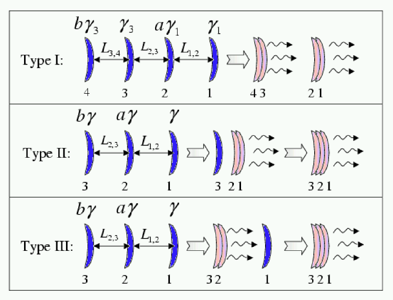
Figure 1: The basic types of multiple collisions.

2.2.1 Interval between consequent pulses

Type I collisions result in two observed pulses, the first at $t_{2}$ and the second at $t_{4}$. The interval between the pulses, $\Delta t$, would be: $\Delta t\approx t_{4}-t_{2}\approx l_{2}+L_{2,3}+l_{3}+L_{3,4}$. In type II collisions the first pulse is observed at $t_{2}$, and second pulse is observed at $t_{3}$. The interval is: $\Delta t\approx t_{3}-t_{2}\approx l_{2}+L_{2,3}$. In type III collisions the last shell takes over the second one, and the first pulse is observed at $t_{3}$. Then the merged shell takes over the first one releasing another pulse observed at $\sim t_{3}$. Therefore type III collisions, results in a single wide pulse.

All these results are accurate up to an order of $1/a_{i,j}^{2}$, where $a_{i,j}$ is the ratio of the Lorentz factors between the two colliding shells. As long as the collisions are efficient, these results depend weakly on the mass distribution of the shells.

2.2.2 The pulses width

The relevant time scales that determine the pulse width are (Piran, 1999): (i) The angular time, $t_{ang}$, which results from the spherical geometry of the shells: $t_{ang}\approx R_{c}/2\gamma^{2}_{sh}$. (ii) The hydrodynamic time, $t_{hyd}$, which arises from the shell’s width and the shock crossing time: $t_{hyd}\approx l_{c_{in}}$, where $l_{c_{in}}$ is the width of the inner shell at the time of the collision. (iii) The cooling time - the time that it takes for the emitting electrons to cool. For synchrotron emission with typical parameters of internal shocks this time is much shorter then $t_{ang}$ and $t_{hyd}$ (Kobayashi et. al. 1997, Wu & Fenimore 2000). Therefore under the assumption of transparent shells the pulse width is $\delta t\approx t_{ang}+t_{hyd}$.

Unlike the pulse’s timing, the pulse’s width depends strongly on the shells’ masses. The relevant Lorentz factor for the calculation is the one of the shocked, and therefore radiating, region - $\gamma_{sh}$. $\gamma_{sh}$ depends strongly on the ratio of the shells’ masses. We examine two possible cases: equal mass shells and equal energy shells. Table 1 summarizes the intervals and the pulses’ width for the two different mass distributions for the three types of collisions.

		Equal mass		Equal energy
	$\Delta t$	$\delta t_{1}$	$\delta t_{2}$	$\delta t_{1}$	$\delta t_{2}$
Type I	$l_{2}+L_{2,3}+l_{3}+L_{3,4}$	$l_{c_{2}}+\frac{L_{1,2}}{a}$	$l_{c_{4}}+\frac{L_{3,4}}{b}$	$l_{c_{2}}+L_{1,2}$	$l_{c_{4}}+L_{3,4}$
Type II	$l_{2}+L_{2,3}$	$l_{c_{2}}+\frac{L_{1,2}}{a}$	$l_{c_{3}}+\frac{L_{1,2}}{b\sqrt{a}}+\frac{L_{2,3}\sqrt{a}}{b}$	$l_{c_{2}}+L_{1,2}$	$l_{c_{3}+}\frac{\sqrt{2}}{5}L_{1,2}+L_{2,3}$
Type III	$\frac{L^{\prime}_{1,2}}{(ab-1)}$	$l_{c_{3}}+\frac{L_{2,3}}{a}$	$>a\sqrt{\frac{a}{b}}L_{2,3}+\frac{L^{\prime}_{1,2}\sqrt{ab}}{(ab-1)}$	No efficient collisions

Table 1: $\Delta t$, and $\delta t$ for the three collisions types for the equal energy/mass shells. In each case there are two pulses. $\delta t_{1}$ [$\delta t_{2}$] is the width of the first [second] observed pulse. $l_{i}$ and $l_{c_{i}}$ are the width at the ejection and width at the collision of the i’th shell ($l_{i}=l_{ci}$ with no spreading.). $L^{\prime}_{1,2}$ is the separation between the first and the second shells at the time that the second and the third shells collide. The approximation here are valid when the Lorentz factors ratio between the colliding shells is larger then 2.

t

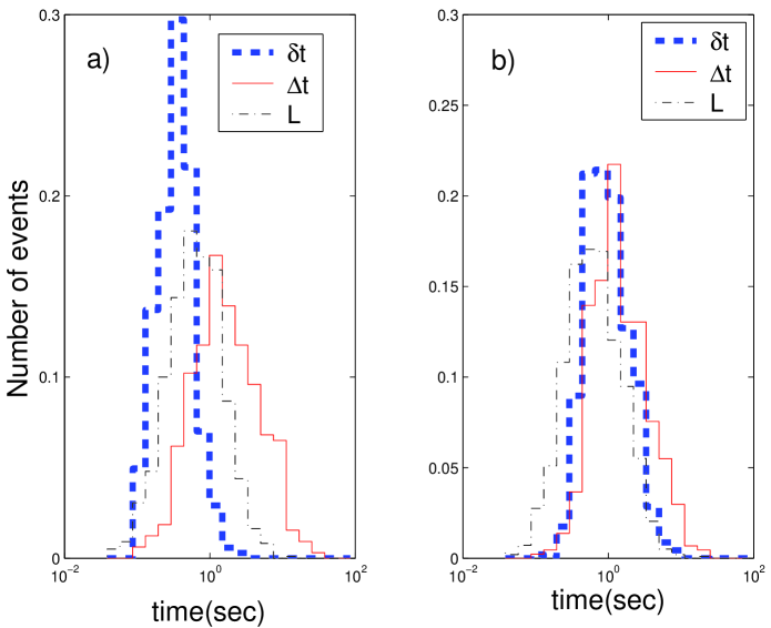
Figure 2: Pulses width, $\delta t$, intervals between pulses, $\Delta t$, and the separation between shells, $L$. (a) : Equal mass shells. (b): Equal energy shells.

3 Numerical Simulation

The toy model demonstrates that the properties of the light curve depend on the dominant type of collisions. In order to determine what are the dominant collisions types we performed numerical simulations of internal shocks light curves. These simulations also enable us to verify some of the approximations used in the analytic toy model.

Following Kobayashi et. al. (1997) each shell is defined by four parameters $\gamma_{i},\,m_{i},\,l_{i}$ and $L_{i,i+1}$. The distribution of the separation between the shells, $L$, is taken to be lognormal with $\mu(ln(L))=-0.5$ and $\sigma(ln(L))=0.9$ (chosen in order to fit the observations). The initial shells width is taken as a constant of 0.1lsec and we assume that the shells do not spread ($l_{c}=l$). The Lorentz factor distribution is uniform ($\gamma_{min}=30$, $\gamma_{max}=2000$). The shells’ mass is either constant (equal mass model) or proportional to $\gamma^{-1}$ (equal energy model).

Each simulation included 50 shells. Following the shell’s motion we identify the collisions. Each collision produce a pulse. The duration of a pulse is taken as $t_{ang}+t_{hyd}$. All the pulses has a fast rise slow decay shape with a ratio of 3:1 between the decay and the rise times. The area below a pulse equals to its radiated energy (no assumption is made here about the efficiency). Using these pulses we prepare a binned (64ms time bins) light curve. We analyze this light curve using the Li & Fenimore (1996) peak finding algorithm, obtaining the observed pulses timing and width.

3.1 Numerical Results

In both models the number of observed pulses is between a third and a half of the total shells emitted. Types I & II collisions are the dominant types (about 80%) in the simulations. The total efficiency in both models is about 20-30%. The equal mass model prefers type I collisions while the equal energy model prefer type II collisions. Efficient type III collisions almost don’t exist in the equal energy model.

Figure 2 illustrates the histograms of the pulses width, $\delta t$, the interval between pulses, $\Delta t$, and the separation between shells, $L$. In the equal mass model (fig. 2a) there is no $\Delta t$-$\delta t$ similarity. $\Delta t$ reflects the $L$ distribution while $\delta t$ is much shorter and does not reflects $L$. In the equal energy model (fig. 2b) both distributions of $\Delta t$ and $\delta t$ reflects the ‘inner engine’ shells separation distribution. Both distributions are consistent with a log normal distribution and the best fits parameters are described in table 2.

	$\Delta t\,(sec)$		$\delta t\,(sec)$
	$\mu$	$1\sigma$	$\mu$	$1\sigma$
Simulated	1.4	0.6-3.4	1	0.5-2
Observed	1.3	0.5-3.1	1	0.5-2.2

Table 2: Best fit parameters of the pulses’ widths and the intervals in the equal energy model, compared to the observed values ( Nakar & Piran 2001). Note that this fit was achieved by tuning only $\mu(ln(L))$ and $\sigma(ln(L))$.

Both results are in a perfect agreement with the analytical results obtained in section 2. The similarity between the “observed” interval distribution in both models is explained by the weak dependence of the pulses’ timing on the mass distribution. The pulses width in the equal energy model reflection of the shells initial separation, $L$, are explained by the analytical result $\delta t\propto L$. The deviation from a lognormal distribution and the short pulses in the equal mass model are explained by the analytical result $\delta t\propto L/a$.

Nakar & Piran (2001) find a correlation between an interval duration and the following pulse. In the equal energy model we find a highly significant correlation between the interval duration and the following pulse. There is no significant correlation in the equal mass model. This result is explained again by the equal mass relation $\delta t\propto L/a$. As the variations in $a$ are larger then the variations in $L$ it wipe out the correlation.

4 Discussion

Former numerical simulations of internal shocks have shown that the resulting light curves reflect the activity of the inner engine. We have shown that this feature arise from the fact that the pulse timing is approximately equal to the ejection time of one of the colliding shell. Moreover, in most collisions (Types I & II) the pulses are distinguishable and each pulse reflects a single collision. In all models the number of observed pulses is 30%-50% of the number of ejected shells. Therefore the light curve reflects the emission time of one third to one half of the shells. The ‘inner engine’ is slightly more variable then the observed light curve.

The observed similarity between the $\Delta t$ and $\delta t$ distributions is explained naturally in the equal energy shells’ model. Both parameters reflects the the separation between the shells during their ejection. In the equal mass shells’ model only $\Delta t$ reflects the initial shells’ separation and therefore such a similarity is not expected.

Our numerical simulations confirmed these predictions. Note that many of the simplifying assumptions can be relaxed with no significant change in the results. We present elsewhere a more detailed model and more elaborated simulations (Nakar & Piran, 2002). The equal energy model simulations fit the observations very well. These results imply that the ‘inner engine’ ejects, most likely, equal energy shells. These results are yet another strong support to the Internal Shock model. They also give one of the first clues on the nature of the ‘inner engine’.

This research was supported by a US-Israel BSF grant.

References

- (1) Kobayashi S., Piran T. & Sari R., 1997, ApJ, 490, 92
- (2) Li H. & Fenimore E., 1996, ApJ, 469, L115
- (3) Nakar, E. & Piran, T., 2001, MNRAS in press (astro-ph/0103210)
- (4) Nakar E. & Piran, T., 2002 in preperation
- (5) Piran, T., 1999, PhR, 314, 575
- (6) Ramirez-Ruiz E. & Fenimore E. E., 2000, ApJ, 539, 712
- (7) Wu, B., & Fenimore, E., 2000 ApJ, 535, L29